Article

Analysis of the Shear Stresses in a Filling Line of Parenteral Products: The Role of Fittings

1
Department of Applied Science and Technology, Politecnico di Torino, 24 Corso Duca degli Abruzzi, 10129 Torino, Italy
2
GSK, 89 Rue de l’Institut, 1330 Rixensart, Belgium
*
Author to whom correspondence should be addressed.
Processes 2023, 11(6), 1797; https://doi.org/10.3390/pr11061797
Submission received: 11 April 2023 / Revised: 31 May 2023 / Accepted: 9 June 2023 / Published: 13 June 2023
(This article belongs to the Section Pharmaceutical Processes)

Abstract

:
Fill-finish of parenteral formulations represents a crucial step in the pharmaceutical industry that necessitates careful monitoring of product stability down the line. Shear stress and interfacial stress are two elements that threaten product stability, the respective contributions of which are still up for debate. This article focuses on the analysis of shear stress in the sampling phase of the filling line. Specifically, Computational Fluid Dynamics (CFD) simulations were employed to determine the shear stress distribution experienced by a protein-based parenteral drug as it passes through sampling fittings of various shapes under laminar and turbulent regime conditions. Rather than seeking the specific mechanism triggering the destabilization of a product, an attempt was made to analyze the fluid dynamics within these fittings and offer further understanding of the resulting shear stress. In addition, information was collected on the product path within the fittings, which allowed the identification of equations suitable for describing the shear stress distribution. The proposed approaches made it possible to consider the actual flowrate subjected to a given shear stress at a given time. Finally, a comparison was drawn with respect to the fluid dynamics within classical straight tubing to outline differences. This study revealed that the shear stress experienced within the fittings was higher than that in the tubing. Moreover, significant differences were reported in the T-fitting case under turbulent conditions.

Graphical Abstract

1. Introduction

Drug manufacturing generally refers to the industrial-scale production of pharmaceutical drugs. It can be broken down into a series of unit operations, of which fill-finish is considered the most critical [1]. Here, the bulk material is filled into smaller vials or syringes [2] that guarantee product integrity and enable subsequent transportation and storage [3]. Fill-finish poses many challenges, including maintaining the quality and stability of the target product [4]. During fill-finish, parenteral protein drug products can be exposed to various stress conditions [3], such as temperature changes, shear forces, interfacial stresses, and changes in ionic strength, which appear to contribute to protein instability [5,6]. Among these, shear forces have recently gained interest as a topic for investigation in the field of pharmaceutical stability because of the obvious need to consider fluid transport phenomena in filling lines.
In particular, shear stress is caused by friction between fluid particles due to the dynamic fluid viscosity ( μ ). In the case of a Newtonian fluid under laminar conditions in one-dimensional systems, it is expressed as follows:
σ = μ   d u d x
where σ has measure of force per unit area (Pa). A relevant role is played by the velocity gradient, d u d x , also referred to as shear rate ( γ ), which has units of inverse time (s−1) [7].
The actual impact of shear stress on the stability of pharmaceutical products is still debated, and controversial theories have arisen. Earlier experiments in shear-induced degradation were conducted by Charm and Wong [8,9]. Using a capillary device, they tested several enzymes (e.g., fibrinogen and catalase) under shear stress. They verified that the products suffered denaturation even at significantly low values of shear rate (10 s−1). In addition, they found that the duration of stress application ( τ ) played a determining role. Therefore, they introduced a quantity, later identified as “shear history” ( S H ), to quantify shear stress as a function of residence time [7]:
S H = γ · τ
Other studies found little or no evidence for shear-induced deactivation for catalase, urease, and cytochrome c, for shear rate values lower than 10 5 s−1 [10,11]. Therefore, they raised the hypothesis that in previous works, deactivation was more due to interfacial phenomena than shear stress. Indeed, it is difficult to isolate the contribution of shear stress from interfacial stress, which has been extensively studied instead [12,13,14]. Furthermore, in a study conducted by Murphy et al. [15], higher shear rates were investigated, reaching up to 10 6 s−1. It was observed that under these conditions, aggregation of monoclonal antibodies was detected. Another recently popular theory holds that product instability is more due to the combined effect of interfacial and shear stress, and it is unlikely that shear stress alone causes protein aggregation [16,17]. While interfaces play an important role in protein adsorption, unfolding, and film formation, shear forces could release aggregates in the bulk solution and, hence, renew the available surface [3]. In this controversial landscape, it becomes necessary to characterize the shear stress distribution in bioprocessing units.
Several methods can be used to evaluate shear stress, allowing experimental or numerical determination. On the one hand, the former assesses wall shear stress based on temperature or fluid velocity profiles but generally shows drawbacks that limit their use on large scales, such as high sensitivity to external noise for real-time probes [18]. On the other hand, numerical methods are based on the use of Computational Fluid Dynamics (CFD) modeling [19]. Among other benefits, these methods can provide full-field data, do not involve product consumption, and help monitor the process in consideration. This enables improvements and troubleshooting [19].
A pivotal role in fill-finish manufacturing is played by product sampling [20]. It may be necessary for a variety of purposes, including pre-qualification, acceptance of consignments, and in-process control. In a manufacturing filling line, the sampling withdrawal is generally performed using two-outlet fittings, whose working principle is later explained in Section 3.
In the present work, numerical modeling of flow through sampling fittings of two different shapes under laminar and turbulent conditions was conducted since limited studies are available in the literature. First, an analysis of the residence times of the particles flowing through the fittings was carried out to deeply investigate and characterize the fluid dynamics. Afterward, multiple approaches were proposed to assess the average shear stress within the fittings. Finally, comparisons were drawn with respect to the shear stress distribution within straight tubing [21] in order to outline potential differences.

2. Governing Equations and Theoretical Background

The velocity and pressure fields can be determined in a CFD simulation by solving the continuity equation and the Navier–Stokes equation. In the case of incompressible fluids, they read as follows:
u i x i = 0
u i t + u j u i x j = 1 ρ p x i + ν   2 u i x j 2
where u i is the ith component of the fluid velocity, p is the fluid pressure, and ρ and ν are its density and kinematic viscosity, respectively.
In the present work, both laminar and turbulent flows were investigated. For the treatment of the latter cases, RANS (Reynolds Averaged Navier–Stokes) modeling was selected and coupled with the κ ω   S S T (Shear Stress Transport) turbulence model. In this model, κ is the turbulent kinetic energy, and ω is the specific turbulent dissipation rate [22]. This model combines the best of the κ ε and κ ω models. This treatment was already employed in a previous work from our research group, where more details about the transport equations for the turbulent properties may be found [21].
Analytical equations for velocity and shear stress profiles in circular tubing under laminar and turbulent conditions were used for numerical validation, as later described in Section 3. Under laminar conditions, the radial velocity may be expressed as a simple function of the distance from the center ( r ), and similarly for the radial shear stress:
u l a m = 2 u ¯ 1 r 2 R 2
σ = Q 4 μ π R 4 r
where u ¯ is the average fluid velocity (m s−1), R is the tubing radius, and Q is the volumetric flowrate (m3 s−1).
When the flow regime is turbulent, instead, random and chaotic changes in pressure and flow velocity arise [23]. The radial velocity is therefore described as:
u t u r b = u m a x 1 r R 1 / n
where n is a function of R e [24].
Furthermore, an equation for the wall shear stress under turbulent conditions was developed as a function of the skin friction factor ( C f ) [25]:
σ t o t a l ,   w a l l = 1 2 ρ u ¯ 2 C f
which, in turn, can be calculated from Prandtl’s friction law for smooth pipes [23].

3. Numerical Set Up

In the present work, we conducted a numerical investigation of the shear stress distribution of a fluid flowing through various fittings via CFD simulations. As mentioned in the Introduction, two-outlet fittings are generally used to allow product sampling. During normal operation, one of the two outlets is blocked, and the product can thus flow to subsequent equipment. When sampling is needed, however, the product flow is stopped and directed to a sampling bag through the previously blocked outlet. Two simplified geometries representing two possible different structure configurations of the sampling lines were considered. The analyzed geometries are shown in Figure 1a,b, and the implemented structures are shown in Figure 1c,d.
The solution of the equations reported in Section 2 is implemented using the finite volume method-based open-source code OpenFOAM 9 (https://github.com/OpenFOAM/OpenFOAM-9 (accessed on 1 January 2022)). The hardware used to run the simulations is an HP workstation with eight logical processors and 16 GB of RAM. Python 3.8 was used for the post-processing of the simulations.
An incompressible and Newtonian fluid was considered, and gravity was neglected. Steady state simulations were chosen for both laminar and turbulent regimes because of their simpler setup and lower computing costs. The meshing procedure made use of the snappyHexMesh utility from OpenFOAM. In the case of the more complex Y-fitting under laminar and turbulent conditions, the background mesh was designed on the Ansys Fluent mesher (Ansys, Inc., Canonsburg, PA, USA).
The length of the arms on T- and Y-fittings with an internal diameter of 9.53 mm was chosen to ensure fully developed flow in both fluid dynamic regimes. This choice was made to prevent any unphysical description in the system due to the proximity of the system boundary conditions [26]. Velocities of 0.042 and 0.500 m s−1 were arbitrarily chosen among the ranges of possible flowrates industrially used for these systems in order to explore both laminar and turbulent conditions, respectively [27]. Under laminar conditions, for example, a low velocity was deliberately chosen to ensure that, after flow deviation, no turbulence would develop due to an increase in velocity.
The domains were discretized by structured grids comprised of hexahedral, prismatic, and polyhedral cells.
The aforementioned κ ω   S S T turbulence model was implemented while using y + insensitive wall functions. For reference, the boundary conditions for the turbulent properties were chosen as presented in Table 1, where β is a turbulent model constant and equals 0.075 and y w is the distance to the first cell center normal to the wall [28].
The chosen turbulence model allows the y + insensitive wall treatment. In fact, it contains wall functions that are valid throughout the whole boundary layer. One of the main advantages of this model is that it is very flexible since it is independent of the y + value. Therefore, precise resolution of the grid in the boundary layer is not needed.
Special attention should be paid to the boundary conditions, which are summarized in Table 2. Besides the conventional boundary conditions for the main patches, the “symmetry” condition was applied to the patch “end”, referring to the clamped exit. This was chosen to mirror the field pattern along such a patch.
Using a Semi-Implicit Method for Pressure-Linked Equations, the OpenFOAM solver simpleFoam was employed. The Geometric Agglomerated Algebraic Multigrid (GAMG) solver was chosen for pressure, while a smooth solver coupled with the Gauss–Seidel smoother was set for the other variables.
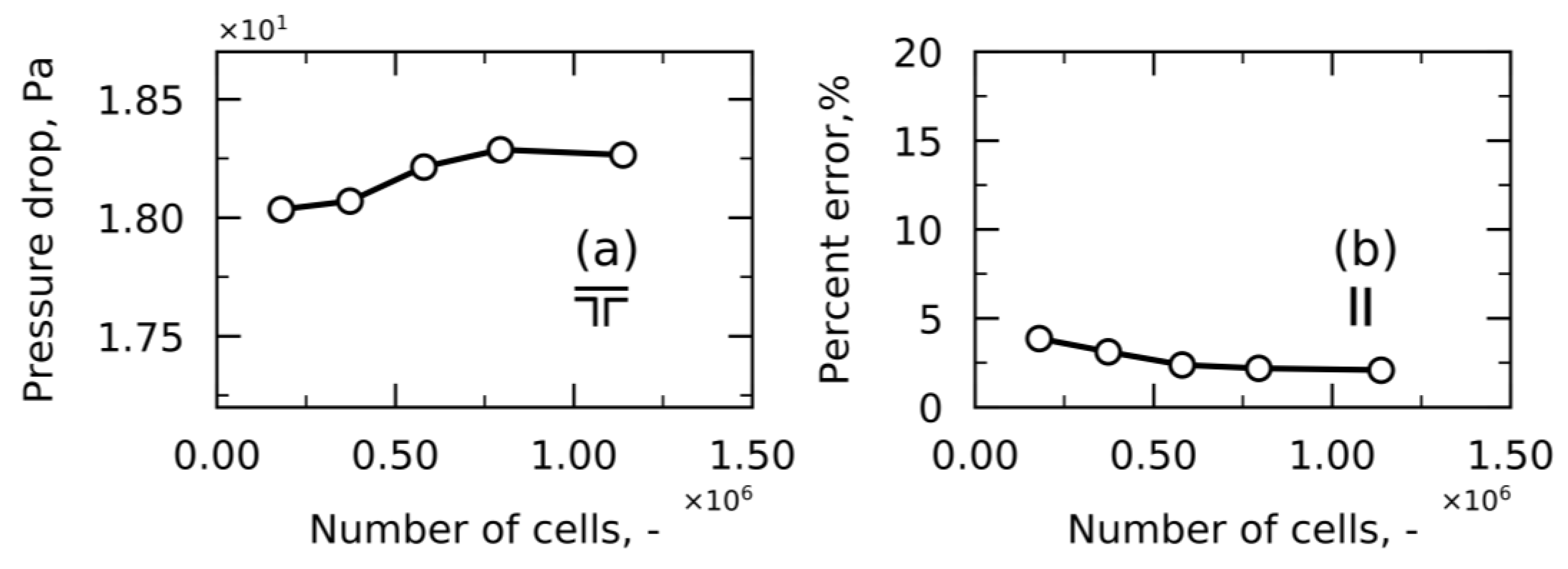
Numerical verification and validation were performed for each geometry and regime condition. Specifically, numerical verification is conducted to make sure that the equations are solved in the right way and is generally conducted through a mesh independence analysis. On the other hand, the numerical validation is carried out by comparing the results of the simulations with experimental values, if any [29]. As reported in the Introduction, several methods can be used for the experimental determination of shear stress. However, these methods have certain limitations that restrict their applicability. For this reason, numerical validation in this study was carried out by comparing the results of the simulations with the well-known equations for the wall shear stress in the straight part of the fitting, where the fluid dynamics develop as in straight tubing.. The grid independence analysis was performed by playing with some parameters. These parameters include the number of background cells in the initial blockMesh, the number of refinement levels close to the wall, and the number of cells between adjacent levels. This analysis confirmed that the solution remained invariant when the mesh was tightened. Finally, the outcome of the simulations was compared with the analytical equations presented in Section 2 as part of the numerical verification. The steps are summarized in Figure 2a,b, which show the numerical validation and verification analyses for a T-fitting in laminar flow. The grid independence analysis in this study involved monitoring the pressure drop across the fitting (Figure 2a). On the other hand, Figure 2b plots the percent error between the numerical and analytical shear stress in the inlet branch of the fitting, where the fluid dynamics develop as in straight tubing. It should be noted that this last analysis was not performed on the entire fittings because no valid analytical equations were found for these geometries.
It can be observed from Figure 2a that the grids comprised more than 0.79 × 10 6 cells led to an almost invariant solution. Increasing the cell number up to the final considered grid led to a small improvement in the solution accuracy, which is not worth the much higher computational demand. A similar trend can be observed in Figure 2b.
A similar approach was taken for numerical verification and validation for the Y-fitting under laminar conditions (Figure S1) and for both fittings under turbulent conditions (Figures S2 and S3). For the Y-fitting under laminar conditions, a mesh with 0.88 × 10 6 cells was chosen. Under turbulent conditions, meshes with about 2.9 × 10 6 and 1.2 × 10 6 cells were chosen for the T- and Y-fitting, respectively.
Furthermore, the mesh quality and topological coherence of the mesh were analyzed using OpenFOAM utilities. This analysis ensured that the mesh adhered to grid quality standards in terms of non-orthogonality (below 75), skewness (below 20 for boundaries and below 4 for internal mesh), and aspect ratio.
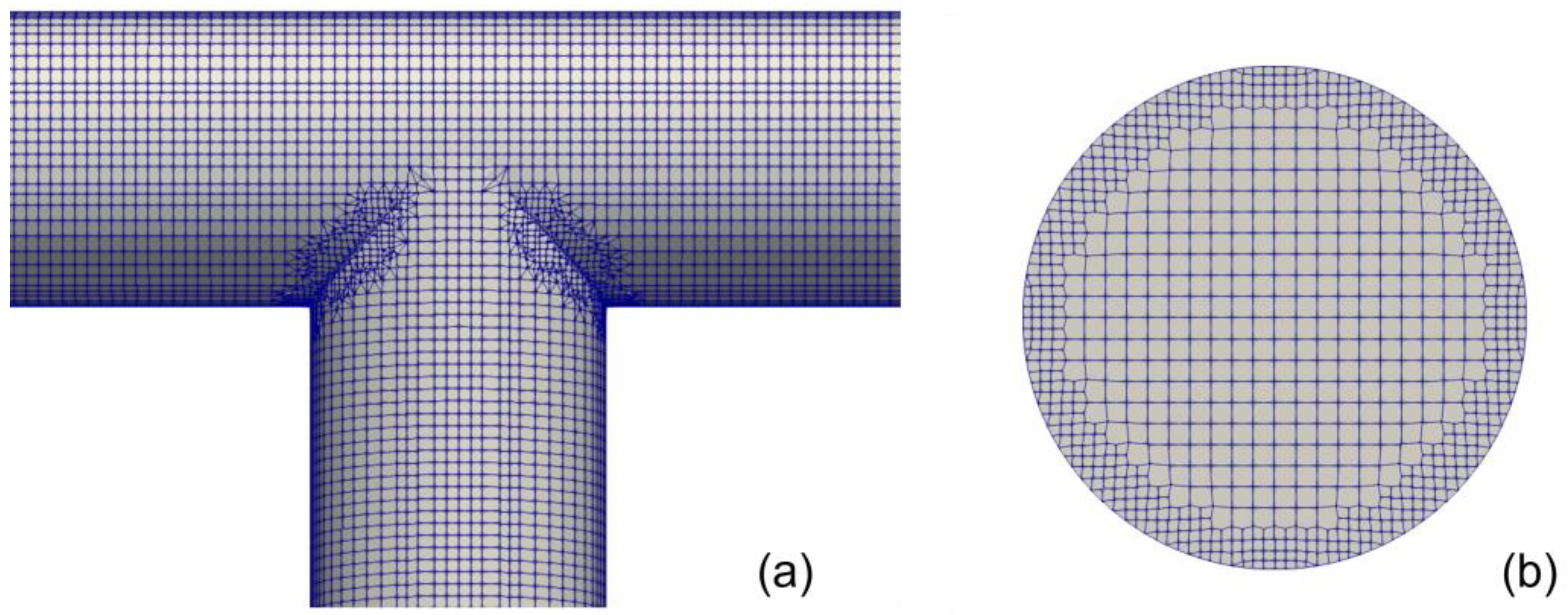
Some images of the chosen grid for the T-fitting under laminar conditions are displayed in Figure 3, where both the outer mesh and the inlet patch mesh are reported for reference.
A similar mesh was chosen for the Y-fitting under laminar conditions and is shown in Figure S4. In the case of T- and Y-fittings under turbulent conditions, instead, layers were added close to the wall, and the resulting meshes are displayed in Figures S5 and S6.
Once the optimal grid was selected and the simulation ran, the ParaView (version 56) application [30] was used to track the trajectories of tracers through the flow. The Stokes number ( S t ) for the fluid particles was initially calculated, which correlates the particle response time and the fluid time scale as follows:
S t = τ P τ f
In the present work, the biological particles in the fluid have about the density of water [31], and their size is smaller than 200   nm [32]. This results in S t below unity for all the operating conditions here described. Therefore, particles are expected to follow fluid streamlines closely. Under such conditions, the particles are governed by advection, and the effect of gravity is neglected. Having made these assumptions, the present work proposes the study of the time evolution of the position and fluid dynamic condition of these tracers as if they were particulate flow parcels. Their tracking was made possible by the use of the “Stream Tracer with Custom Source” algorithm available in ParaView. This is similar to Lagrangian particle tracking but does not take into account diffusive and dispersive phenomena. For ease of reference, these particulate flow parcels will be referred to as “particles” throughout the manuscript.
The algorithm implemented in ParaView works by taking a set of points in the data set, called “seed points”, and then integrating the streamlines starting at these points. By definition, streamlines are curves that are instantaneously tangential to the vector field in the dataset. In particular, they indicate the direction in which the particles in the dataset would travel at that instant of time [33]. The streamline integration was tuned by choosing a “forward” direction and a maximum streamline length. The latter parameter was chosen high enough so as to follow the complete trajectories of the particles throughout the geometry. The seed point locations were given as input to the integrator, and their release is described in Section 4.1.

4. Results

4.1. Velocity and Residence Time Study

In the studied fittings, the fluid does not flow through the entire geometry. Instead, it is made apparent that there is a zone where particles enter and stay for a long time at a low velocity. If we consider the time scales of vial filling, this zone can be considered a “dead zone” (a zone from which trapped particles will not be released before the filling ends) and will be referred to as such in the present article.
These characteristics differ from the tubing geometry [21], where an integral operation on the domain was sufficient and tracking individual particles and investigating their statistical behavior was not needed. Here, particle tracking through streamlines was necessary and offered fluid dynamics data that integral analyses are unable to provide. Figure 4 shows an instance of fluid dynamics inside the T-fitting (a) and Y-fitting (b) in laminar conditions where 520 particles were followed through their trajectories. It can be observed that a significant number of particles cross the “dead zone”, which is (almost) totally separated from the rest of the domain. In particular, over-analysis of 520 particles under laminar (and turbulent) conditions resulted in the finding that around 5% of the entire flowrate crossed the “dead zone”. This underlines the importance of analyzing these two-outlet fittings rather than pure flow deviators. Particle tracking inside the T- and Y-fittings under turbulent conditions, instead, is displayed in Figure S7.
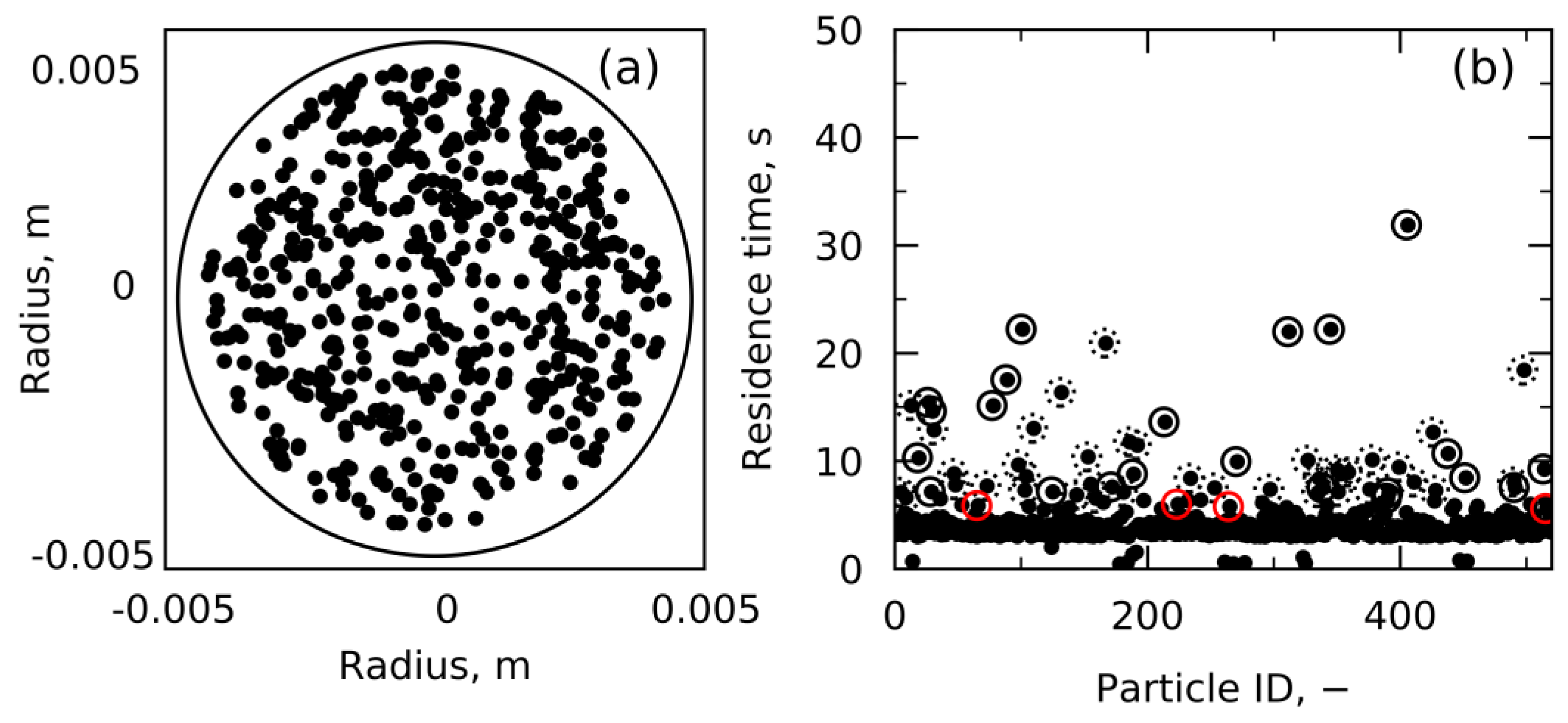
Finding the optimal quantity of particles to release was the subject of an initial inquiry. Due to postprocessing requirements, the particles were dispersed at random throughout a circle with a diameter equal to 90% of the tubing’s diameter, as shown in Figure 5a. This decision was supported by the fact that only a small proportion of the formulation flows in the near-wall region, which is characterized by the lowest fluid velocities. Figure 5b displays the residence time of 520 particles released from the inlet of the fitting. It can be observed that, in this particular case (velocity of 0.042 m s−1), the majority of particles take between 1 and 6 s to cross the domain, while some particles take substantially longer—between 6 and 40 s. These high residence time values are caused by particles passing through the dead zone, indicated by the black solid circles in Figure 5b. Additionally, particles that deviate from their original direction and come close to the wall experience the no-slip condition, entering the lower velocity boundary layer and are indicated by the dotted circles. For the sake of clarity, particles passing through the dead zone with a residence time lower than 6 s are also identified by the red solid circles in the same figure. The upper limit used for this analysis, i.e., 6 s, was identified using the Tukey test [34].
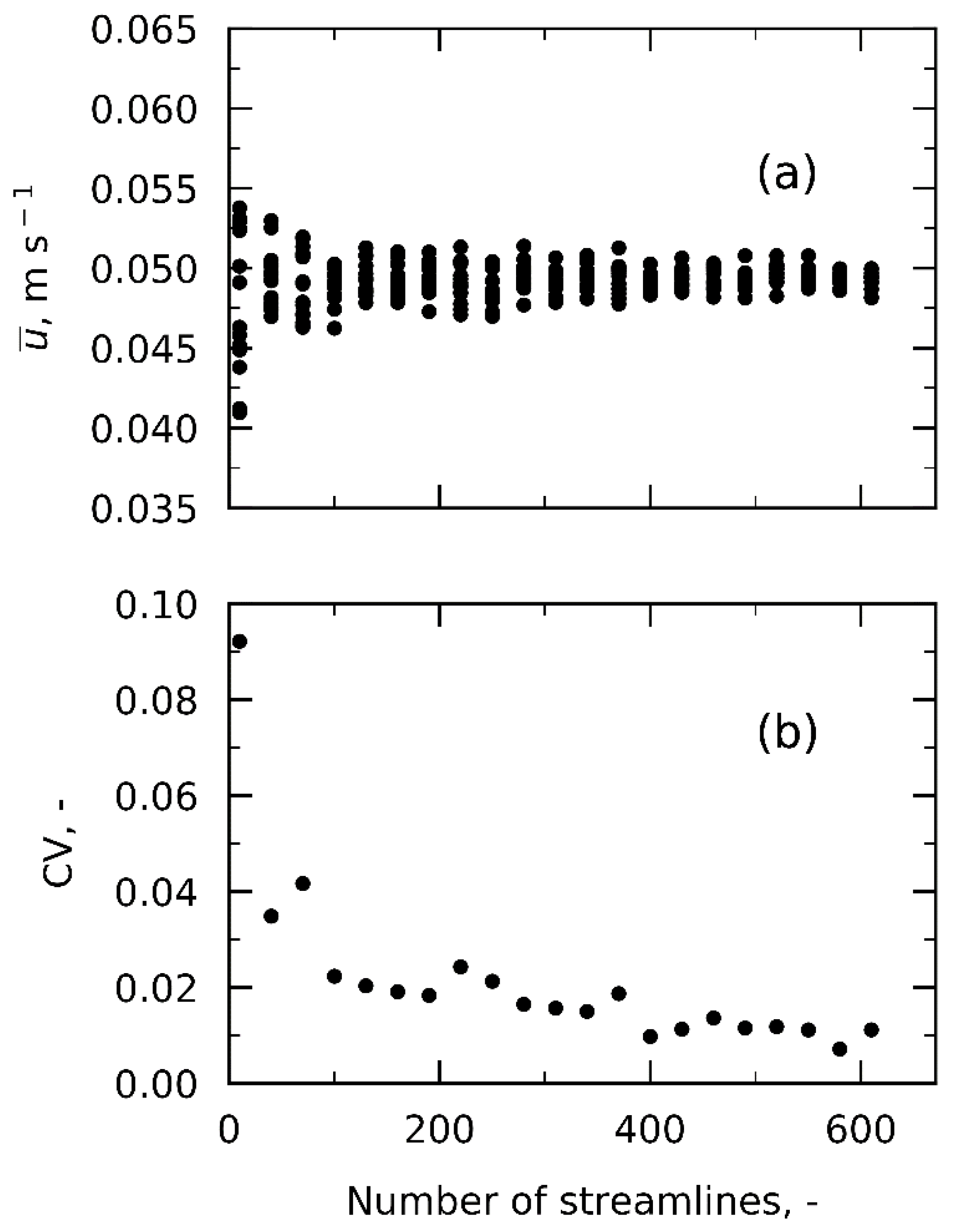
The optimal number of particles to release was obtained by monitoring the average velocity, as illustrated in Figure 6a. It was calculated by averaging the velocities of all the streamlines. In turn, the velocity for each streamline i was assessed as follows:
u i = 1 τ i 0 τ i u i t   d t
where t is the time step, τ i is the overall particle residence time, and u i t is the velocity at the relevant time step.
Between 10 and 610 particles were discharged from the fitting inlet. A total of 15 tests with varying (but still random) particle layouts were run at fixed particle numbers to control for statistical variance. For clarity, the coefficients of variation ( C V ) are shown in Figure 6b. As it can be observed, the C V (defined as the ratio between the standard deviation and the average value) stabilized at very low values, under 2%, as the number of particles, and therefore streamlines, rose. Although values over 300 can be thought of as optimal, 520 particles were chosen because the increase in particles did not result in an appreciable increment in computational expense. The average inlet velocity in this test was set at 0.042 m s−1. The average velocity in Figure 6a is slightly higher because particles were released onto a surface that was smaller than the actual tubing surface, thus ignoring some of the slowest particles.

4.2. First Case Study: Laminar Flow

4.2.1. Shear Stress Distribution

The flow deviation causes noticeable local velocity gradients, which are visible in Figure 4 and explained in Section 4.1, resulting in shear stress. To refer to the shear stress of a filling line operating unit, reference is often made to the maximum shear stress [17]. However, these values are unrealistic for characterizing the shear stress distribution because they overestimate it [21,35], resulting in incorrectly quantifying the effect of shear stress on product stability.
Consequently, an effort was made to develop approaches to appropriately quantify average shear stress and give a more realistic picture.

Approach 1—Maximum Shear Stress per Streamline

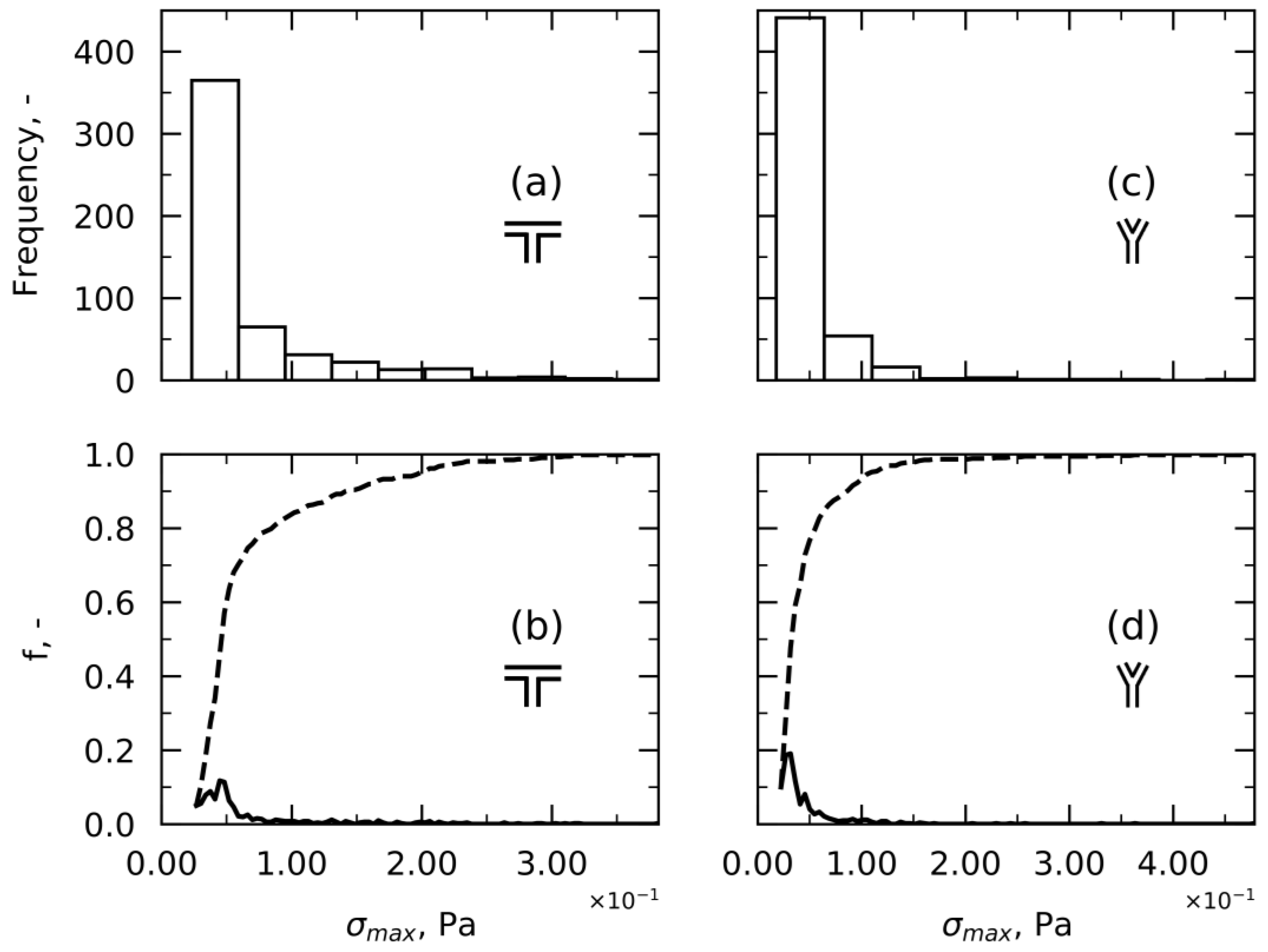
The highest shear stress for each streamline is taken into account in the first conservative approach. For simpler result visualization, probability distributions were employed [36]. Frequency histograms, Probability Distribution Function ( P D F ) and Cumulative Distribution Function ( C D F ) for the highest shear stress in the T-fitting are shown in Figure 7a,b, respectively.
Figure 7c,d shows a similar trend for the Y-fitting. Sturges’ rule was used to determine the number of bins in Figure 7a,c [37], while Figure 7b,d uses 100 bins, allowing for a clearer representation.
This strategy is not only conservative—since it only considers the highest shear stress per particle along its trajectory—but it also does not account for how long a particle experiences a specific shear stress. However, as noted in the introduction, residence time appears to be important. As a result, new definitions were developed.

Approach 2—Damage Factor

A new quantity called damage factor ( D F ) was introduced, drawing on earlier works [8]. Following Equation (11), DF for the streamline i takes into account the local shear rate γ and the relative time of exposure τ for each streamline. By employing this approach, D F becomes dimensionless and gives a quantitative idea of the cumulative damage to the product.
D F i = 0 τ i γ i t   d t
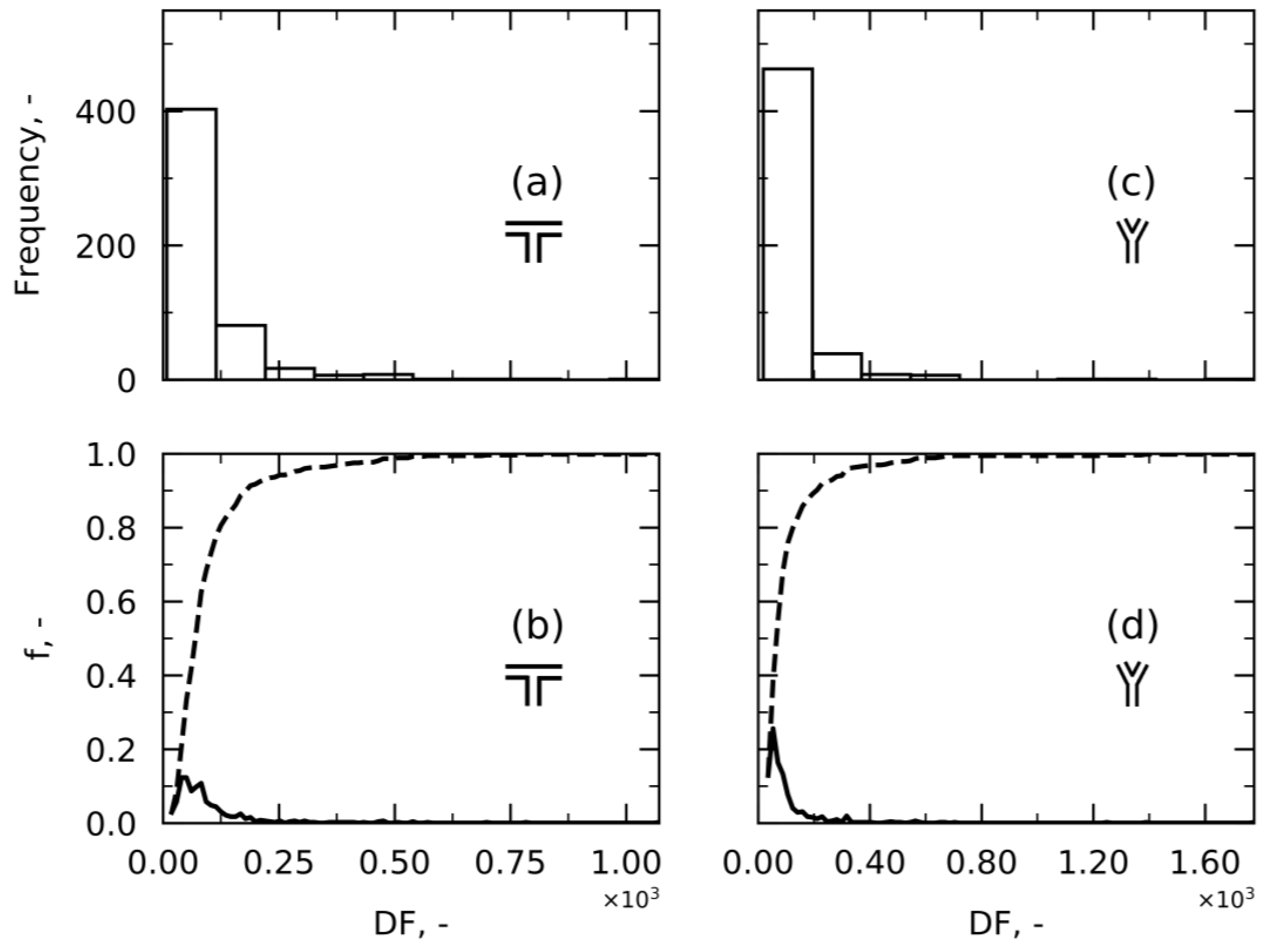
The trapezoidal rule was used to estimate the integral [38], using as the resolution of partition the time step of the integrator selected in ParaView. Figure 8 depicts the findings of this approach for T- and Y-fittings under laminar conditions in terms of the probability distribution for easier understanding. It is clear that most streamlines have a low D F , but a few have a significantly larger D F . In order to determine which particles were causing such high D F values, we carried out a further examination. It was found that, despite experiencing small shear stress, particles with a large residence time (introduced in Section 4.1) and a relatively low shear rate can result in high values of D F . These high D F values, however, are not representative because it is reasonable to assume that particles that experience low shear stress for a long period of time do not contribute as much to damage as particles subjected to high shear stress for short periods.

Approach 3—Damage Fitting Factor

It can be assumed that there is a threshold below which it is pointless to “count” the shear stress’ contribution to damage. Therefore, it was decided to introduce one such arbitrary threshold. Thus, we have chosen to have a shear account for the accumulation of damage only when its value is greater than the maximum shear rate in fitting-equivalent tubing ( γ t ) . Damage fitting factor ( D F F ) is the name of this factor, and the formula is as follows:
D F F i = 0 τ i Γ i t   d t
where
Γ i t 0                   i f   γ i t γ t γ i t       i f   γ i t > γ t
Results for T- and Y-fittings under laminar conditions are reported in Figure S8. This method allows low-shear stress to be neglected. However, it is still very sensitive to the particles’ residence time and domain size since it is a cumulative function and not an average.

Approach 4—Damage Critical Factor

Approach 4 is very similar to Approach 3 but introduces a different threshold. As explained in the Introduction, it was suggested that shear rate only becomes significant when it exceeds a critical value, and many authors attempted to identify this key value.
D C F i = 0 τ i Γ i t   d t
where
Γ i t 0                   i f   γ i t γ c γ i t       i f   γ i t > γ c
Here, Equation (14) can be used to determine the damage critical factor ( D C F ) for a specified product, where γ c is represented by its critical shear rate, if any such threshold is identified. To provide an example, γ c was chosen to be 30% of the fitting’s maximum shear rate.
The results of the application of Approach 4 for T- and Y-fittings under laminar conditions are reported in Figure S9. The comparison between Approaches 2, 3, and 4 for T- and Y-fittings under laminar conditions is presented in Table 3. To allow for comparison, average quantities were calculated among all the streamlines.
When a threshold to the shear rate is introduced ( D F F ¯ , D C F ¯ ), the cumulative damage decreases within both shapes of the fitting. However, it is not possible to make a direct comparison between T- and Y-fittings under the same fluid dynamic regime because these damage factors are closely related to domain size. A higher damage factor is not necessarily due to higher stress but perhaps to a larger domain and thus longer paths to the product. These considerations highlight the need for a definition based on average rather than cumulative functions to facilitate qualitative and quantitative comparisons, which still take into account shear stress peaks.

Approach 5—Time-Averaged Shear Stress

The shear stress per streamline is time-averaged across its trajectory as follows:
σ i = 1 τ i 0 τ i σ i t   d t
The trapezoidal rule was then used to estimate the integral [38], using as the resolution of the partition the time step of the integrator selected in ParaView. The average shear stress is then calculated as follows:
σ ¯ 5 = 1 m i   σ i
where m is the number of streamlines.
The results of this approach are presented in the next paragraph, where a comparison with Approach 6 is outlined.

Approach 6—Time-Averaged Shear Stress weighted on Flowrates

In line with the results reported in our earlier study [21], an even more realistic measure of the average shear stress can be obtained by weighting the local shear stresses on the relative flowrates. Since particles are released randomly from the fitting inlet, this weighting operation is equivalent to sending particles in a proportional amount to the actual flowrate. As reported in Section 4.1, the optimal number of particles to release was assessed by monitoring the average velocity through the fitting. Hence, since the chosen number is guaranteed to describe the whole fluid dynamics within the fitting, the area of influence of the individual streamlines ( A i ) was given by the ratio of the cross-sectional area to the number of streamlines. As a result, Approach 6 was developed as follows:
σ ¯ 6 = i 1 τ i 0 τ i σ i t   d t · w i w t o t
where the local weights corresponded to the relative flowrates and were evaluated as:
w i = A i 1 τ i 0 τ i u i t   d t
with u being the velocity at the relevant time step and i being the streamline index.
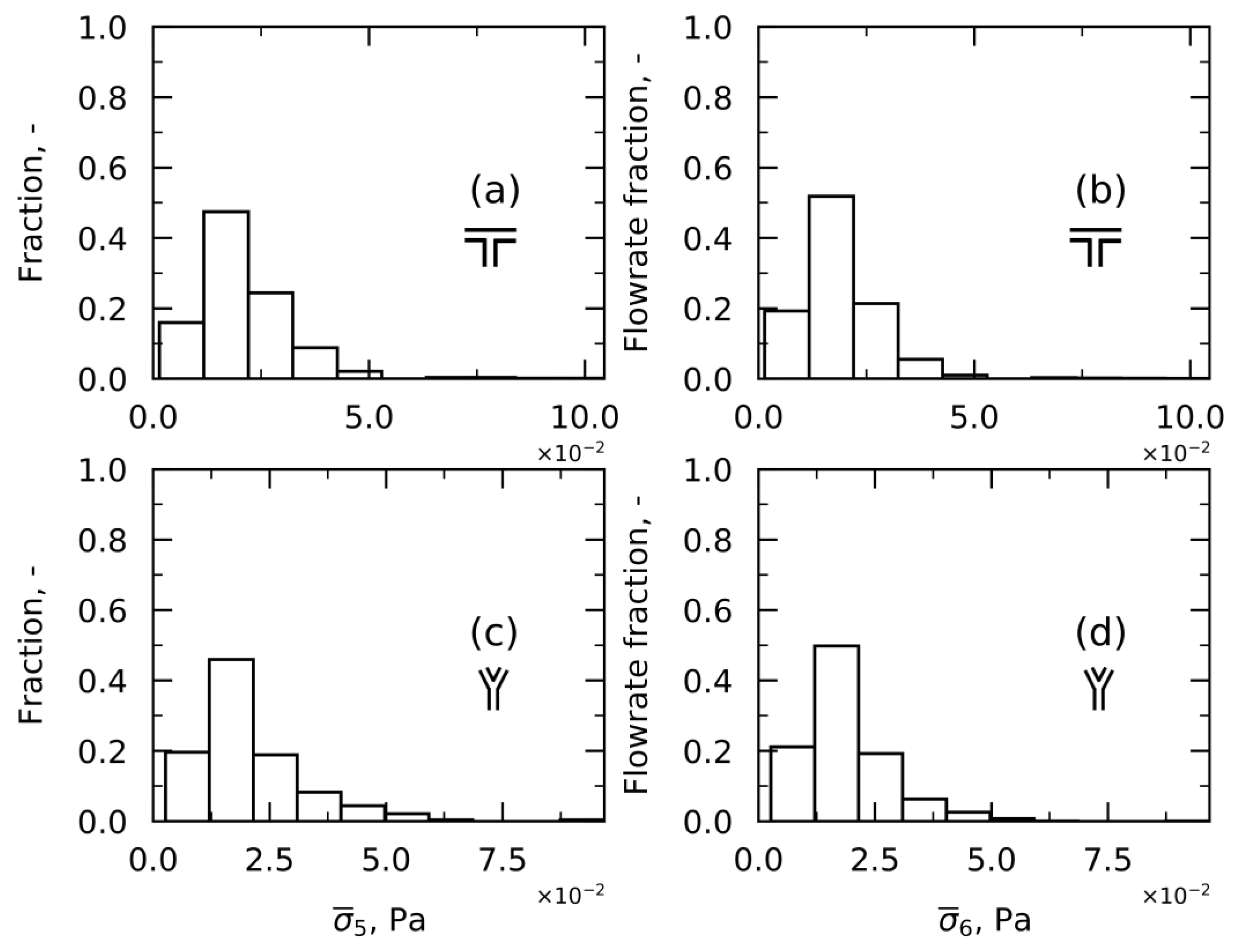
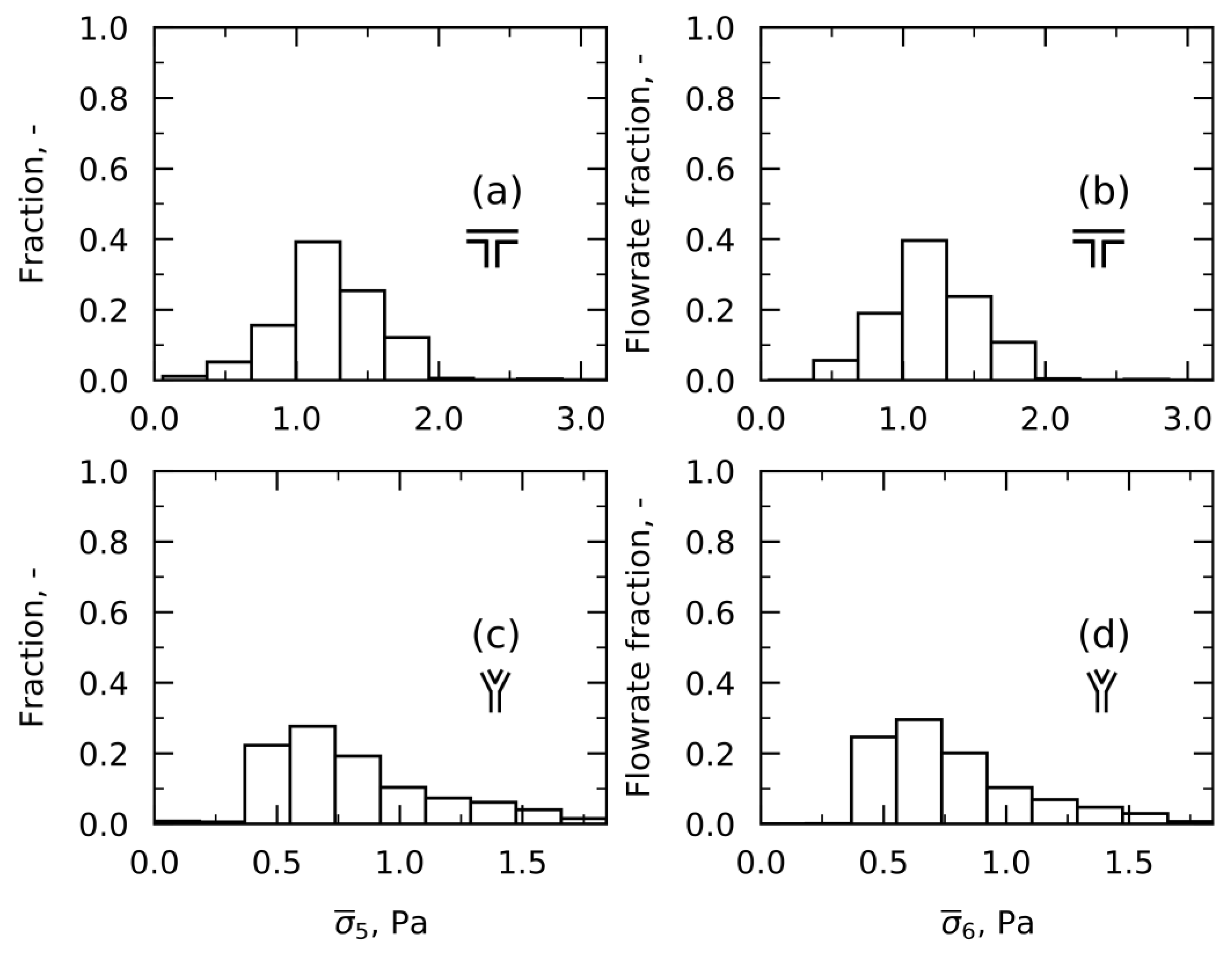
Figure 9 presents the comparison between Approaches 5 and 6 under laminar conditions for T- and Y-fittings.
The main difference between the two approaches is evident when examining the near-zero shear bars for T-fitting in Figure 9a,b (or Y-fitting in Figure 9c,d). When Approach 6 is used, these bars are shifted towards higher values on the y-axis, which means that their weight is worth more. This is because Approach 6 allows the shear contributions to be considered proportionally to how much product actually passes through the fitting at the various locations, i.e., the local volumetric flowrate.

4.3. Second Case Study: Turbulent Flow

Similar investigations to those reported under the laminar regime were conducted for T- and Y-fittings under turbulent conditions. The mathematical details for the proposed equations are already presented in Section 2. Here, the relevant results are shown, and a comparison with respect to the laminar flow is drawn.

Shear Stress Distribution

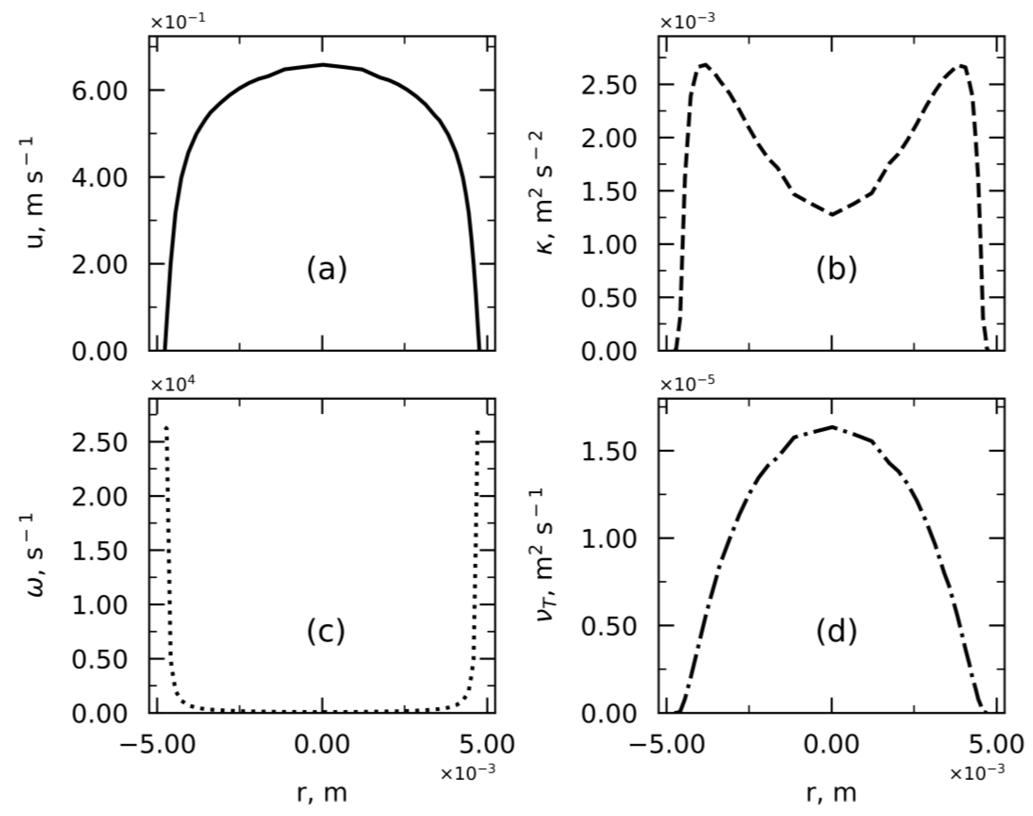
Accurate analysis of the mesh layout was conducted in the framework of the κ ω   S S T turbulent model. The turbulent properties in the inlet branch of the fitting, where the fluid dynamics develop as in straight tubing, varied as displayed in Figure 10.
By monitoring the local properties within the fittings, peaks in shear stress were found as a result of the abrupt change of direction of the flow. The aforementioned Approaches 1 to 4 were used to describe the distribution of shear stress. The results are presented in Figures S10–S13 and Table S1. In a similar fashion to what is reported in Section 4.2.1, Approach 1 appeared too conservative, while Approaches 2, 3, and 4 did not allow precise comparison because they were too dependent on domain size. Again, Approaches 5 and 6 proved suitable to describe the relationship between shear stress and residence time. Their comparison is shown in Figure 11.
Similar considerations for the comparison between Approaches 5 and 6 can be drawn for turbulent flow. By weighting the local shear stresses on the volumetric flowrate fraction, the average shear stress decreases because the higher shear stresses are experienced by a small portion of the entire product and vice versa, which can be noted later in Table 4. As for laminar conditions, Approach 6 can provide a more realistic picture of the shear stress distribution.

4.4. Comparison with Shear Stress in Straight Tubing

This article presents new approaches for numerically evaluating the average shear stress across different fittings. Together with our previous article on tubing [21], they provide a new way to quantify the distribution of shear stress (or rates) in a filling line under given operating conditions. However, they differ from the way the models were designed. In the tubing case, under the steady state assumptions, velocity and shear stress profiles did not change along the length of the tubing. Therefore, integral operations over a slice of the tubing were sufficient. However, in a fitting, the deviation of the flow direction caused the particles to differ from their stationary trajectories. This is the reason why the shear was evaluated along the particle’s trajectories and the relevant variables detected.
For a clearer representation, Table 4 summarizes the relevant results. Using the models developed in the previous article [21], the average shear stress weighted on the local flowrates ( σ ¯ t u b ) was calculated. Then, it was compared with the value calculated using Approaches 5 and 6 for fitting, σ ¯ 5 ,   f i t and σ ¯ 6 ,   f i t , respectively. A new quantity ( Δ t u b , f i t ) was identified and calculated as follows:
Δ t u b , f i t = σ ¯ t u b σ ¯ 6 ,   f i t σ ¯ t u b
It can be observed that in the T-fitting under laminar conditions, the difference Δ t u b , f i t in the average shear stress (between σ ¯ t u b   and σ ¯ 6 ,   f i t ) is rather small. On the other hand, Δ t u b , f i t is much higher in the T-fitting under turbulent conditions. As for the Y-fitting, under both laminar and turbulent conditions, Δ t u b , f i t is smaller or equivalent to the T-fitting. This may be explained by the fact that the change in flow direction is not as sharp.
The models presented show that in a filling line consisting of tubing and fittings, the fittings represent the largest source of shear stress. Under turbulent flow conditions, in particular, the difference between the average shear stresses generated in the T-fittings and tubing becomes even more significant. This highlights the relevance of the present work. Nonetheless, for the other fitting shape analyzed, i.e., Y-fitting, the discrepancy is not as significant.
Finally, in a filling line comprised of a defined number of fittings, Approach 6 could be implemented to realistically quantify the average shear stress experienced by the product when flowing through the fitting.

5. Conclusions

In the present work, CFD simulations were employed to investigate the fluid dynamics within T- and Y-fittings under both laminar and turbulent conditions. The potential streamlines of particles were tracked to gain more insights into the fluid path and detect local properties. Several relations were then proposed to identify the shear stress distribution. Particularly, one was identified (Approach 6), which turned out to be the most suitable for our purposes and takes into account the local shear stresses along the particle’s trajectory and the relative flowrates. This helps to provide a more realistic picture of the shear stress distribution since it is equivalent to considering particles in a proportional way to their actual amount. In a broader perspective, the same workflow and approach for evaluating the shear stress distribution could be used on fittings or connectors of different shapes as well as other operating units.
The future steps of this study could involve (i) extending the analysis on shear stress to the other components present in a filling line for parenteral protein drug products and (ii) performing experimental tests to assess the impact of such shear stress on product stability.

Supplementary Materials

The following supporting information can be downloaded at: https://www.mdpi.com/article/10.3390/pr11061797/s1, Figure S1: Numerical verification and validation analyses for Y-fitting under laminar conditions: grid independence analysis (a), the percent error between the numerical and analytical shear stress in the inlet branch of the fitting (where the fluid dynamics develop as in a tubing) is monitored by varying the number of cells (b); Figure S2: Numerical verification and validation analyses for T-fitting under turbulent conditions: grid independence analysis (a), the percent error between the numerical and analytical shear stress in the inlet branch of the fitting (where the fluid dynamics develop as in a tubing) is monitored by varying the number of cells (b); Figure S3: Numerical verification and validation analyses for Y-fitting under turbulent conditions: grid independence analysis (a), the percent error between the numerical and analytical shear stress in the inlet branch of the fitting (where the fluid dynamics develop as in a tubing) is monitored by varying the number of cells (b); Figure S4: Details of the mesh for Y-fitting under laminar conditions: outer mesh (a) and inlet patch mesh (b); Figure S5: Details of the mesh for T-fitting under turbulent conditions: outer mesh (a) and inlet patch mesh (b); Figure S6: Details of the mesh for Y-fitting under turbulent conditions: outer mesh (a) and inlet patch mesh (b); Figure S7: A total of 520 particles are followed through their streamlines, and their trajectories and velocities are displayed for T-fitting (a) and Y-fitting (b) under turbulent conditions; Figure S8: Frequency histograms of the D F F for T- (a) and Y- (c) fittings under laminar conditions. P D F (continuous line) and C D F (dotted line) are also presented for T- (b) and Y- (d) fittings; Figure S9: Frequency histograms of the D C F for T- (a) and Y- (c) fittings under laminar conditions. P D F (continuous line) and C D F (dotted line) are also presented for T- (b) and Y- (d) fittings; Figure S10: Frequency histograms of the maximum shear stress for T- (a) and Y- (c) fittings under turbulent conditions. P D F (continuous line) and C D F (dotted line) are also presented for T- (b) and Y- (d) fittings; Figure S11: Frequency histograms of the D F for T- (a) and Y- (c) fittings under turbulent conditions. P D F (continuous line) and C D F (dotted line) are also presented for T- (b) and Y- (d) fittings; Figure S12: Frequency histograms of the D F F for T- (a) and Y- (c) fittings under turbulent conditions. P D F (continuous line) and C D F (dotted line) are also presented for T- (b) and Y- (d) fittings; Figure S13: Frequency histograms of the D C F for T- (a) and Y- (c) fittings under turbulent conditions. P D F (continuous line) and C D F (dotted line) are also presented for T- (b) and Y- (d) fittings; Table S1: Comparison in D F ¯ , D F F ¯ , D C F ¯ for T- and Y-fittings under turbulent conditions.

Author Contributions

C.M., B.S., E.B., G.B. and R.P. were involved in the conception and design of the study. C.M., B.S., G.B. and R.P. were involved in the selection of the study methodology. C.M. performed the CFD simulations. C.M., B.S. and M.B. analyzed and interpreted the results. C.M. wrote the first draft of the manuscript. All authors were involved in drafting the manuscript or revising it critically for important intellectual content. All authors had full access to the data and approved the manuscript before it was submitted by the corresponding author. All authors have read and agreed to the published version of the manuscript.

Funding

This work was sponsored and financially supported by GlaxoSmithKline Biologicals SA.

Data Availability Statement

Not applicable.

Conflicts of Interest

The authors declare the following competing financial interest(s): B.S., M.B. and E.B. are employees of the GSK group of companies. C.M. holds a Doctorate studentship and collaborates with GSK as part of her Ph.D. training.

Nomenclature

A streamline area of influence, m2
C f skin friction factor, -
C V coefficient of variation, -
D C F damage critical factor, -
D F damage factor, -
D F F damage fitting factor, -
k turbulent kinetic energy, m2 s−2
m number of streamlines, -
n factor, -
p fluid pressure, Pa
Q volumetric flowrate, m3 s−1
r distance from the center, m
R tubing radius, m
R e Reynolds number, -
S t Stokes number, -
S H shear history, -
t time, s
u fluid velocity, m s−1
u ¯ average fluid velocity, m s−1
u t friction velocity, m s−1
w volumetric flowrate weight, m3 s−1
x spatial coordinate, m
y absolute distance from the wall, m
y + sub-layer scaled distance, -
y w distance to the first cell center normal to the wall, m
Greek letters
β turbulent model constant, -
γ shear rate, s−1
Δ difference, -
ε turbulent dissipation rate, m2 s−3
κ turbulent kinetic energy, m2 s−2
μ dynamic fluid viscosity, kg m−1 s−1
ν kinematic viscosity, m2 s−1
ν T turbulent kinematic viscosity, m2 s−1
ρ fluid density, m3 kg−1
σ shear stress, Pa
τ residence time, s
Γ filtered shear rate, s−1
τ f fluid time scale, s
τ p particle response time, s
ω specific turbulent dissipation rate, s−1
Subscripts
f i t fitting
i index
j index
l a m laminar
m a x maximum
t o t total
t u b tubing
t u r b turbulent
w a l l wall
Abbreviations
CDFCumulative Distribution Function
CFDComputational Fluid Dynamics
GAMGGeometric Agglomerated Algebraic Multigrid
PDFProbability Distribution Function
RANSReynolds Averaged Navier–Stokes
SSTShear Stress Transport

References

  1. Kovarcik, D.P. Critical Factors for Fill–Finish Manufacturing of Biologics. Bioprocess International. 17 May 2016. Available online: https://bioprocessintl.com/manufacturing/fill-finish/critical-factors-for-fill-finish-manufacturing-of-biologics/ (accessed on 10 March 2022).
  2. Martagan, T.; Akcay, A.; Koek, M.; Adan, I. Optimal production decisions in biopharmaceutical fill-and-finish operations. IISE Trans. 2020, 53, 149–163. [Google Scholar] [CrossRef]
  3. Das, T.K.; Sreedhara, A.; Colandene, J.D.; Chou, D.K.; Filipe, V.; Grapentin, C.; Searles, J.; Christian, T.R.; Narhi, L.O.; Jiskoot, W. Stress Factors in Protein Drug Product Manufacturing and Their Impact on Product Quality. J. Pharm. Sci. 2022, 111, 868–886. [Google Scholar] [CrossRef] [PubMed]
  4. Shire, S.J. Monoclonal Antibodies: Meeting the Challenges in Manufacturing, Formulation, Delivery and Stability of Final Drug Product; Woodhead Publishing: Cambridge, UK, 2015. [Google Scholar]
  5. Niazi, S. Pharmaceutical Manufacturing Formulations; Pharmaceutical Scientist, Inc.: Deerfield, IL, USA, 2009; Volume 6. [Google Scholar]
  6. Lapidus, L.J. Protein unfolding mechanisms and their effects on folding experiments. F1000Research 2017, 6, 1723. [Google Scholar] [CrossRef] [PubMed] [Green Version]
  7. Bekard, I.B.; Asimakis, P.; Bertolini, J.; Dunstan, D.E. The effects of shear flow on protein structure and function. Biopolymers 2011, 95, 733–745. [Google Scholar] [CrossRef] [PubMed]
  8. Charm, S.E.; Wong, B.L. Enzyme inactivation with shearing. Biotechnol. Bioeng. 1970, 12, 1103–1109. [Google Scholar] [CrossRef]
  9. Charm, S.E.; Wong, B.L. Shear degradation of fibrinogen in the circulation. Science 1970, 170, 466–468. [Google Scholar] [CrossRef]
  10. Thomas, C.R.; Dunnill, P. Action of shear on enzymes: Studies with catalase and urease. Biotechnol. Bioeng. 1979, 21, 2279–2302. [Google Scholar] [CrossRef]
  11. Jaspe, J.; Hagen, S.J. Do protein molecules unfold in a simple shear flow? Biophys. J. 2006, 91, 3415–3424. [Google Scholar] [CrossRef] [Green Version]
  12. Arsiccio, A.; McCarty, J.; Pisano, R.; Shea, J.E. Heightened Cold-Denaturation of Proteins at the Ice-Water Interface. J. Am. Chem. Soc. 2020, 142, 5722–5730. [Google Scholar] [CrossRef]
  13. Arsiccio, A.; McCarty, J.; Pisano, R.; Shea, J.E. Effect of Surfactants on Surface-Induced Denaturation of Proteins: Evidence of an Orientation-Dependent Mechanism. J. Phys. Chem. B 2018, 122, 11390–11399. [Google Scholar] [CrossRef]
  14. Arsiccio, A.; Pisano, R. The Ice-Water Interface and Protein Stability: A Review. J. Pharm. Sci. 2020, 109, 2116–2130. [Google Scholar] [CrossRef]
  15. Murphy, R.P.; Riedel, Z.W.; Nakatani, M.A.; Salipante, P.F.; Weston, J.S.; Hudson, S.D.; Weigandt, K.M. Capillary RheoSANS: Measuring the rheology and nanostructure of complex fluids at high shear rates. Soft Matter 2020, 16, 6285–6293. [Google Scholar] [CrossRef]
  16. Nesta, D.; Nanda, T.; He, J.; Haas, M.; Shpungin, S.; Rusanov, I.; Sweder, R.; Brisbane, C. Aggregation from Shear Stress and Surface Interaction: Molecule-specific or universal phenomenon? Bioprocess International. 17 April 2017. Available online: https://bioprocessintl.com/analytical/pre-formulation/aggregation-shear-stress-surface-interaction-molecule-specific-universal-phenomenon/ (accessed on 16 November 2021).
  17. Bee, J.S.; Stevenson, J.L.; Mehta, B.; Svitel, J.; Pollastrini, J.; Platz, R.; Freund, E.; Carpenter, J.F.; Randolph, T.W. Response of a concentrated monoclonal antibody formulation to high shear. Biotechnol. Bioeng. 2009, 103, 936–943. [Google Scholar] [CrossRef] [Green Version]
  18. Winter, K.G. An outline of the techniques available for the measurement of skin friction in turbulent boundary layers. Prog. Aerosp. Sci. 1979, 18, 1–57. [Google Scholar] [CrossRef]
  19. Pordal, H.S.; Matice, C.J.; Fry, T.J. The role of computational fluid dynamics in the pharmaceutical industry. Pharm. Technol. 2002, 26, 72–79. [Google Scholar]
  20. WHO. Annex 4 WHO Guidelines for Sampling of Pharmaceutical. WHO Guidel. Sampl. Pharm. Prod. Relat. Mater. 2005, 929, 61–93. Available online: https://apps.who.int/iris/bitstream/handle/10665/43157/WHO_TRS_929_eng.pdf (accessed on 15 December 2021).
  21. Moino, C.; Scutellà, B.; Bellini, M.; Bourlès, E.; Boccardo, G.; Pisano, R. Analysis of the Shear Stresses in a Filling Line of Parenteral Products: The Role of Tubing. Processes 2023, 11, 833. [Google Scholar] [CrossRef]
  22. Menter, F.R. Two-equation eddy-viscosity turbulence models for engineering applications. AIAA J. 1994, 32, 1598–1605. [Google Scholar] [CrossRef] [Green Version]
  23. Pope, S.B. Turbulent Flows; Cambridge University Press: Cambridge, UK, 2000. [Google Scholar]
  24. Schlichting, H. Boundary Layer Theory, 7th ed.; McGraw-Hill, Inc.: New York, NY, USA, 1979. [Google Scholar]
  25. Kudela, H. Turbulent Flow and Turbulence Modeling. Notes 2011, 1–48. Available online: http://www.itcmp.pwr.wroc.pl/~znmp/dydaktyka/fundam_FM/Lecture_no3_Turbulent_flow_Modelling.pdf (accessed on 24 February 2022).
  26. Tu, J.; Yeoh, G.-H.; Liu, C. Computational Fluid Dynamics, 3rd ed.; Elsevier Ltd.: Amsterdam, The Netherlands, 2018. [Google Scholar]
  27. Byron Bird, R.; Stewart, W.E.; Lightfoot, E.N. Transport Phenomena, 2nd ed.; John Wiley & Sons, Inc.: New York, NY, USA, 2002. [Google Scholar]
  28. Guerrero, J. OpenFOAM Advanced Training. Turbulence Modeling in General CFD and OpenFOAM—Theory and Applications. 2022. Available online: http://www.wolfdynamics.com/tutorials.html?id=120 (accessed on 22 July 2022).
  29. Versteeg, H.K.; Malalasekera, W. An Introduction to Computational Fluid Dynamics, 2nd ed.; Pearson Education, Inc.: Harlow, UK, 2007. [Google Scholar]
  30. Ayachit, U. The ParaView Guide: A Parallel Visualization Application; Kitware Inc.: Clifton Park, NY, USA, 2018; p. 274. Available online: https://www.mn.uio.no/astro/english/services/it/help/visualization/paraview/paraviewguide-5.6.0.pdf (accessed on 20 September 2022).
  31. Fischer, H.; Polikarpov, I.; Craievich, A.F. Average protein density is a molecular-weight-dependent function. Protein Sci. 2009, 13, 2825–2828. [Google Scholar] [CrossRef]
  32. Bachmann, M.F.; Jennings, G.T. Vaccine delivery: A matter of size, geometry, kinetics and molecular patterns. Nat. Rev. Immunol. 2010, 10, 787–796. [Google Scholar] [CrossRef]
  33. Moreland, K. The ParaView Tutorial; National Technology and Engineering Solutions of Sandia LLC: Mountain View, CA, USA, 2014. [Google Scholar]
  34. Tukey, J.W. Exploratory Data Analysis; Addison-Wesley Publishing Company: Glenview, IL, USA, 1977. [Google Scholar]
  35. Duerkop, M.; Berger, E.; Dürauer, A.; Jungbauer, A. Influence of cavitation and high shear stress on HSA aggregation behavior. Eng. Life Sci. 2018, 18, 169–178. [Google Scholar] [CrossRef] [PubMed] [Green Version]
  36. Kumar, G.; Banerjee, R.; Kr Singh, D.; Choubey, N.; Arnaw. Mathematics for Machine Learning. J. Math. Sci. Comput. Math. 2020, 1, 229–238. [Google Scholar] [CrossRef]
  37. Scott, D.W. Sturges’ rule. WIRES Comput. Stat. 2009, 1, 303–306. [Google Scholar] [CrossRef]
  38. Atkinson, K.E. An Introduction to Numerical Analysis, 2nd ed.; John Wildey & Sons: Toronto, ON, Canada, 1989. [Google Scholar]
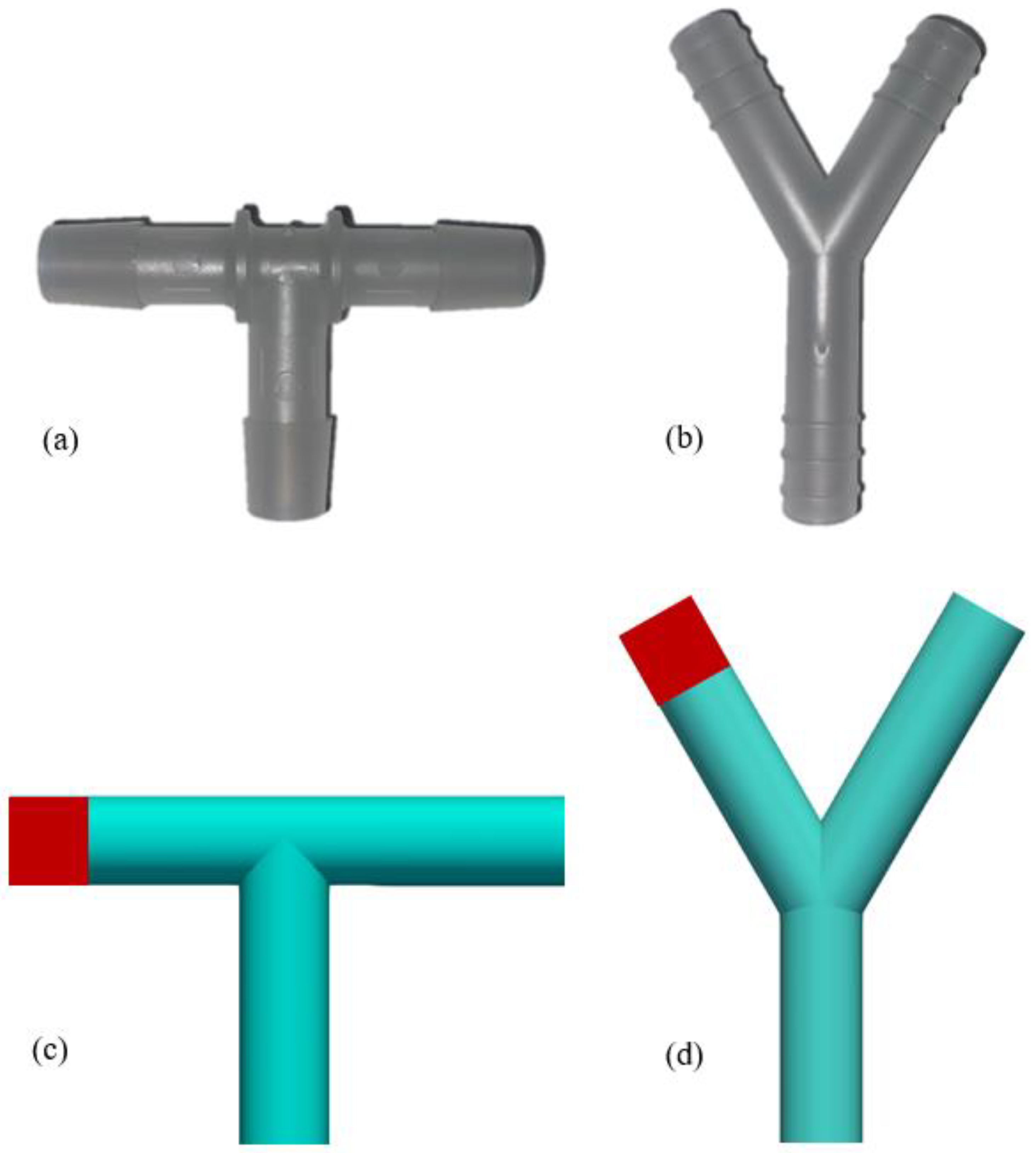
Figure 1. Geometries analyzed. (a,b) display the real geometries focused on in the present study for T- and Y-fittings with an internal diameter of 9.53 mm. (c,d) represent the modeled geometries obtained, where the clamped outlets are colored in red.
Processes 11 01797 g001
Figure 2. Numerical verification and validation analyses for T-fitting under laminar conditions: grid independence analysis (a), the percent error between the numerical and analytical shear stress in the inlet branch of the fitting (where the fluid dynamics develop as in a tubing) is monitored by varying the number of cells (b).
Processes 11 01797 g002
Figure 3. Details of the mesh for T-fitting under laminar conditions: outer mesh (a) and inlet patch mesh (b).
Processes 11 01797 g003
Figure 4. A total of 520 particles are followed through their streamlines, and their trajectories and velocities are displayed for T-fitting (a) and Y-fitting (b) under laminar conditions.
Processes 11 01797 g004
Figure 5. (a) A total of 520 seeds were randomly released at the inlet of the connector on a surface with a diameter equal to 90% of the tubing diameter. (b) Particles’ residence times. As visible from the x scale, 520 particles were released from the inlet of the connector.
Processes 11 01797 g005
Figure 6. Average velocity calculated based on streamline information (a). The related coefficients of variation ( C V ) are reported in (b).
Processes 11 01797 g006
Figure 7. Frequency histograms of the maximum shear stress for T- (a) and Y- (c) fittings under laminar conditions. PDF (continuous line) and CDF (dotted line) are also presented for T- (b) and Y- (d) fittings.
Processes 11 01797 g007
Figure 8. Frequency histograms of the D F for T- (a) and Y- (c) fittings under laminar conditions. P D F (continuous line) and C D F (dotted line) are also presented for T- (b) and Y- (d) fittings.
Processes 11 01797 g008
Figure 9. Average shear stress according to Approach 5 (a) and Approach 6 (b) is monitored by varying the number of streamlines and the number of tests per streamline for T-fitting under laminar conditions. (c,d) refer to Y-fitting.
Processes 11 01797 g009
Figure 10. Velocity profile in the cross-section of the straight part of the connector is shown in panel (a). Trends of turbulent properties κ , ω and ν T are presented in panels (bd), respectively.
Processes 11 01797 g010
Figure 11. Average shear stress according to Approach 5 (a) and Approach 6 (b) is monitored by varying the number of streamlines and the number of tests per streamline for T-fitting under turbulent conditions. Panels (c,d) refer to Y-fitting.
Processes 11 01797 g011
Table 1. Boundary conditions (at the wall and the inflow patch) are expressed in terms of OpenFOAM classes.
Turbulence PropertyBoundary Condition at the WallEstimation
κ fixedValue or kLowReWallFunction 1 × 10 10
ω omegaWallFunction 10 6 ν β y w 2
ν T nutLowReWallFunction 0
Turbulence PropertyBoundary Condition at the Inflow PatchEstimation
κ fixedValue 1 × 10 10
ω fixedValue 10 6 ν β y w 2
ν T calculated 0
Table 2. Boundary conditions for the main patches are expressed in terms of OpenFOAM classes.
Boundary Condition
Patch p u
inletzeroGradient fixedValue   ( u ¯ )
outletuniformValue (0)zeroGradient
wallzeroGradientnoSlip
endsymmetrysymmetry
Table 3. Comparison in D F ¯ , D F F ¯ , and D C F ¯ for T- and Y-fittings under laminar conditions.
Case v ,   m   s 1 D F ¯ , D F F ¯ , D C F ¯ ,
T- 0.042 97.30 33.93 2.89
Y- 0.042 105.10 44.84 0.16
Table 4. Comparison in the shear stress distribution between fitting and tubing [21] under laminar and turbulent conditions.
CaseRegime u ¯ ,   m   s 1 σ ¯ t u b ,   Pa σ ¯ 5 ,   f i t ,   Pa σ ¯ 6 , f i t ,   Pa Δ t u b ,   f i t  
T-Lam 0.042 1.88 × 10 2 2.10 × 10 2 1.92 × 10 2 2 %
Y-Lam 0.042 1.88 × 10 2 2.08 × 10 2 1.89 × 10 2 1 %
T-Turb 0.500 7.69 × 10 1 12.3 × 10 1 12.1 × 10 1 57 %
Y-Turb 0.500 7.69 × 10 1 8.13 × 10 1 7.84 × 10 1 2 %
Disclaimer/Publisher’s Note: The statements, opinions and data contained in all publications are solely those of the individual author(s) and contributor(s) and not of MDPI and/or the editor(s). MDPI and/or the editor(s) disclaim responsibility for any injury to people or property resulting from any ideas, methods, instructions or products referred to in the content.