Material Transport and Flow Pattern Characteristics of Gas–Liquid–Solid Mixed Flows

Abstract

Flow pattern monitoring of gas–liquid–solid mixed flow has great significance to enhance the quality and efficiency of material mixing, and the material transport mechanism and dynamic control strategy are faced with significant challenges. To solve these problems, a computational fluid mechanics and discrete element method (CFD-DEM) coupling modeling and solving approach based on soft sphere and porous models is presented to explore material transport mechanisms. The user-defined function (UDF) is adopted to perform data communication, and the porosity of the porous model is calculated to achieve the bidirectional calculation of Eulerian fluid and Lagrange particle phases. Material transport processes of gas–liquid–solid mixed flows are discussed to explore material transport mechanisms of particle flow and the flow pattern evolution laws under the inflation control are obtained. The results show that the particles are not evenly distributed under the synergistic action of impeller rotation and inflation. The particles in the upper and lower impeller have similar characteristics along the radial direction, and there is an aggregation phenomenon in the impeller center. A certain degree of inflation enhances the macroscopic mixing process of turbulent vortices, promotes the particle suspension effect inside the container, and improves the material transport efficiency inside the mixing space. Relevant research results can provide theoretical references for the material transport mechanism, flow pattern tracking models, and energy transfer and can also provide technical support for chemical process separation, food processing, battery homogenate mixing, and other production processes.

1. Introduction

With the sustained development of industrial production, hybrid technologies have been widely used in civil construction, biopharming, new energy, and petrochemical engineering. Material mixing is an important link that makes the material be distributed more evenly between phases. Gas–liquid–solid mixed flows are critical in high-end chemical, biopharmaceutical, and lithium battery manufacturing. The mixing devices and flow channels must provide high mass transfer and turbulence capacity. The above requirements make mixing courses complex, and it is difficult to observe the whole flow field and particle distribution [1,2,3,4]. The physical scales of the mixed spaces are larger than that of the materials. The complex cyclic and turbulent flow provides critical technical challenges to the optimal design of the mixed actuator and boundary condition control of the mixing process [5,6,7,8].

At present, the computational fluid dynamics (CFD) approach is widely applied to the liquid–solid mixing process. It is generally based on Euler–Euler models, which regard the particle phase as a continuous phase to describe the interphase infiltration process. The model consumes relatively little computational resources, but the simulation accuracy is low. Moreover, particle motion states cannot be obtained [9,10,11,12,13]. The discrete element method (DEM) based on Euler–Lagrange models can obtain the motion and interaction of particles, which can be combined with different fluid dynamics calculation methods to simulate fluid–particle flow [14,15,16]. Delacroix adopted the CFD-DEM model to reproduce various properties in the material mixed system, and verified its effectiveness, which created broad prospects for applying CFD-DEM [17]. Ting et al. adopted CFD-DEM models to study solid suspension behaviors. Compared with experimental measurements and CFD simulation based on the Euler–Euler scheme, CFD-DEM simulation can offer abundant flow field data [18]. Blais et al. proposed the semi-analytical CFD-DEM models and optimized the solid–liquid mixing operation, which increased the particle suspension ratio and improved the flow pattern and particle distribution but did not consider the distribution and stability of the free surface [19,20]. Sun et al. developed an Euler–Lagrange method-based model that can calculate three-phase flow motions [21]. Combining the RSM turbulence model, Kang et al. simulated the particle suspension dynamics in a mixed space with an unblocked flow component. They obtained the influence laws of the channel geometry, impeller speed, particle density, and diameter on the vortices, flow pattern, and material motion [22].

The studies on the multiphase flows concentrate on free-liquid surfaces, flow patterns, and two-phase. Still, it rarely considers the effect of internal inflation on the liquid–solid, especially when the particle phases are regarded as discrete particle phases. Therefore, it is necessary to set up the fluid–solid dynamic model and study the gas–liquid–solid mixed processes to explore action regularities and dynamic control strategies.

Aiming at the above goal, this paper first proposes a gas–liquid–solid mixed flow mechanics model with a CFD-DEM coupling modeling method. It uses a self-developed, user-defined function (UDF) to acquire fluid–particle forces. A novel porous model is utilized to obtain particle trajectories. Finally, the effects of aeration on fluid velocity, flow pattern, and particle suspension are discussed. Relevant research results can provide theoretical references for material transport mechanisms, flow pattern tracking modes, and energy transfer and can also provide technical support for chemical process separation, food processing, battery homogenate mixing, and other production processes.

2. Three-Phase Flow Mechanics Model

2.1. Volume of Fluid Model

There are complex gas–liquid coupling phenomena in the mixing process, so it should be described by a multiphase flow model. The volume of fluid (VOF) model describes a real-time interface characteristic method. The flow features of gas–liquid ingredients and the capture of transient characteristics in the mixing process are calculated, and continuity and momentum equations can be described [23,24,25,26].

$$\frac{\partial {\epsilon }_{\mathrm{f}}}{\partial t}+\nabla \cdot \left({\epsilon }_{\mathrm{f}}\mathit{u}\right)=0$$

(1)

$$\frac{\partial \left({\rho }_{\mathrm{f}}{\epsilon }_{\mathrm{f}}\mathit{u}\right)}{\partial t}+\nabla \cdot \left({\rho }_{\mathrm{f}}{\epsilon }_{\mathrm{f}}\mathit{uu}\right)=-{\epsilon }_{\mathrm{f}}\nabla p+\nabla \cdot ({\epsilon }_{\mathrm{f}}(\mu \left(\nabla \mathit{u}+\nabla {\mathit{u}}^T\right)+{\rho }_{\mathrm{f}}\mathit{g}+{\mathit{F}}_{\mathbf{s}\mathbf{t}}))+{\mathit{F}}_{\mathbf{p}\mathbf{f}}$$

(2)

where ρ_f is the fluid density, ε_f is the void ratio, u is the fluid velocity, F_pf is the reaction force of the interaction term, p is the pressure, μ is the hydrodynamic viscosity, and F_st is the surface tension [27,28,29]. To improve the calculating accuracy and make the calculation closer to the actual situation, the continuum surface force (CSF) model should be adopted. The expression is as follows.

$${\mathit{F}}_{\mathbf{s}\mathbf{t}}=\sigma \mathit{\kappa }\cdot \nabla \varphi$$

(3)

where σ is the surface tension coefficient, and κ is the curvature of the gas–liquid phase interface, its expression is described.

$$\mathit{\kappa }=\frac{1}{\left|\mathit{n}\right|}\left[\left(\frac{\mathit{n}}{\left|\mathit{n}\right|}\cdot \nabla \right)\left|\mathit{n}\right|\right]-(\nabla \cdot \mathit{n})$$

(4)

where n represents the unit normal vector of the interface. For the VOF model, the gas–liquid interface can be solved by the interface transmission equation.

$$\frac{\partial (\alpha )}{\partial t}+\nabla \cdot (\alpha \mathit{u})=0$$

(5)

where α is the volume fraction of the gas phase, if α = 1, the cell represents all gas ingredients; if 0 < α < 1, the cell contains gas and liquid ingredients; if α = 0, the cell is all gas ingredients.

The standard turbulent k-ε model should be selected to solve fluid governing equation to obtain accurate simulation results, which have good computational performance in the violently changing flow field. Its governing equation is as follows [30,31,32,33].

$$\frac{\partial (\rho k)}{\partial t}+\frac{\partial \left(\rho k{u}_i\right)}{\partial x_i}=\frac{\partial }{\partial x_j}\left[\left(\mu +\frac{{\mu }_t}{{\sigma }_k}\right)\frac{\partial k}{\partial x_j}\right]+G_{\mathrm{k}}+G_{\mathrm{b}}-\rho \epsilon -Y_{\mathrm{M}}+S_{\mathrm{k}}$$

(6)

$$\frac{\partial (\rho \epsilon )}{\partial t}+\frac{\partial \left(\rho \epsilon u_i\right)}{\partial x_i}=\frac{\partial }{\partial x_j}\left[\left(\mu +\frac{{\mu }_t}{{\sigma }_{\mathsf{\epsilon }}}\right)\frac{\partial \epsilon }{\partial x_j}\right]+C_{1\mathsf{\epsilon }}\frac{\epsilon }{k}\left(G_{\mathrm{k}}+C_{3\mathsf{\epsilon }}{G}_{\mathrm{b}}\right)-C_{2\mathsf{\epsilon }}\rho \frac{{\epsilon }^2}{k}+S_{\mathsf{\epsilon }}$$

(7)

where k is the turbulence energy, ε is the dissipation rate of turbulence energy, G_b is the turbulence energy generation term, Y_M is the influence of compressible turbulence pulsation expansion on the total dissipation rate, G_k is the turbulence energy generation term, C_1ε, C_2ε, and C_3ε are the empirical constant, and σ_k and σ_ε are the Prandt number.

2.2. Discrete Element Method

DEM can calculate particle flow laws and analyze contact forces and motions of discrete particles. The particle’s motion is calculated based on Newton’s second law, and the relation between the translation and rotation speed and position of the particle with time can be obtained through calculation. The particle translation motions depend on the force summation acting on it, but the contact torque controls the rotational motion. Its governing equation can be expressed as [34,35,36]:

$$m_i\stackrel{••}{{\mathit{x}}_{\mathit{i}}}={\displaystyle \sum _j{\mathit{F}}_{\mathbf{c},\mathit{ij}}}+{\mathit{F}}_{\mathbf{p}\mathbf{f},\mathit{i}}+m_i\mathit{g}$$

(8)

$$I_i\stackrel{••}{{\mathit{\theta }}_{\mathbf{p}.\mathit{i}}}={\displaystyle \sum _j\left({\mathit{T}}_{\mathbf{t},\mathit{ij}}+{\mathit{T}}_{\mathbf{r},\mathit{ij}}\right)}$$

(9)

where F_c,ij denotes the interphase contact force, F_pf,i is the interaction force, g is the gravity acceleration, m_i is the particle mass, x_i is the particle displacement, I_i is the inertia moment, θ_p,i represents the angular displacement, and T_t,ij and T_r,ij are tangential and rolling friction moments. Some forces and torques contained in Equations (8) and (9) are calculated in Equations (10)–(16).

Contact force:

$${\mathit{F}}_{\mathbf{c},\mathit{ij}}={\mathit{F}}_{\mathbf{c}\mathbf{n},\mathit{ij}}+{\mathit{F}}_{\mathbf{c}\mathbf{t},\mathit{ij}}$$

(10)

Normal contact force:

$${\mathit{F}}_{\mathbf{c}\mathbf{n},\mathit{ij}}=\frac{4}{3}{Y}^{*}\sqrt{R^{*}}{\delta }_{\mathrm{cn},ij}^{3/2}+2\sqrt{\frac{5}{6}}\frac{\ln e}{\sqrt{{\ln }^{2}e+{\pi }^2}}\sqrt{S_{\mathrm{cn},ij}{m}^{*}}{\mathit{v}}_{\mathbf{c}\mathbf{n}}$$

(11)

Tangential contact force:

$${\mathit{F}}_{\mathbf{c}\mathbf{t},\mathit{ij}}=-{\delta }_{\mathrm{ct},ij}{S}_{\mathrm{ct},ij}+2\sqrt{\frac{5}{6}}\frac{\ln e}{\sqrt{{\ln }^{2}e+{\pi }^2}}\sqrt{S_{\mathrm{ct},ij}{m}^{*}}{\mathit{v}}_{\mathbf{c}\mathbf{t}}$$

(12)

Tangential friction torque:

$${\mathit{T}}_{\mathit{t},\mathit{ij}}=L_{ij}{\mathit{n}}_{\mathit{ij}}\times {\mathit{F}}_{\mathbf{ct},\mathbf{ij}}$$

(13)

Rolling friction torque:

$${\mathit{T}}_{\mathbf{r},\mathit{ij}}=-{\mu }_r{L}_{ij}\left|{\mathit{F}}_{\mathbf{c}\mathbf{n},\mathit{ij}}\right|\frac{{\mathit{\omega }}_{\mathit{ij}}}{\left|{\mathit{\omega }}_{\mathit{ij}}\right|}$$

(14)

Particle-fluid force:

$${\mathit{F}}_{\mathbf{p}\mathbf{f}}=\frac{1}{\mathbf{\Delta }V}{\displaystyle \sum _i^{n_p}{\mathit{f}}_{\mathbf{p}\mathbf{f},\mathit{i}}}-{\mathit{f}}_{\nabla \mathit{p},\mathit{i}}-{\mathit{f}}_{\nabla \mathit{\tau },\mathit{i}}-{\mathit{f}}_{\mathbf{s}\mathbf{t},\mathit{i}}$$

(15)

$${\mathit{f}}_{\mathbf{p}\mathbf{f},\mathit{i}}={\mathit{f}}_{\mathbf{d},\mathit{i}}+{\mathit{f}}_{\nabla \mathit{p},\mathit{i}}+{\mathit{f}}_{\nabla \mathit{\tau },\mathit{i}}+{\mathit{f}}_{\mathbf{s}\mathbf{t},\mathit{i}}+{\mathit{f}}_{\mathbf{v}\mathbf{m},\mathit{i}}+{\mathit{f}}_{\mathbf{B},\mathit{i}}+{\mathit{f}}_{\mathbf{Saff},\mathit{i}}+{\mathit{f}}_{\mathbf{M}\mathbf{a}\mathbf{g},\mathit{i}}$$

(16)

2.3. An Interphase Coupling-Solving Approach

To acquire accurate interaction forces between fluid and particles, a porous model is put forward to solve particle motions, and its calculation expression is as follows:

$${\epsilon }_f=1-{\displaystyle \sum _i{\epsilon }_{\mathrm{ps},i}}$$

(17)

where ε_ps,i represents the particle volume per unit volume of the first porous ball in the fluid unit. This model overcomes the unstable computation problem induced via the traditional method, as the particle size can be close to the mesh size, improves fluid-particle interactions, and includes particle volumes in the calculation process, so the flow field obtained by this method is more accurate.

The calculation process is shown in Figure 1. The boundary condition of the flow field should be initialized. Then, the velocity and force are obtained through iterative solving of Equations (1) and (2). The change information can be acquired via Equation (5). The velocity and position of particles are obtained by iterative calculation of Equations (8) and (9) and updated by DEM. If not, the voltage of the fluid unit can be obtained by solving Equation (17) in Section 2.3, and the flow calculation above the field can be continued. This two-way coupling can be realized, and data can be exchanged until convergence stops and the simulation is completed.

3. Numerical Calculation

3.1. Physical Model and Grid Division

The limited physical mixing space in this paper contains dual-layer mixing execution components, as shown in Figure 2. The width of the calculation area is 7 m and the height is 15 m. The geometric construction has an air pipeline, impellers, and a drainage pipe. The mixing tank structure, the screw, nut, and mixed tank near impellers are simplified. As the impellers rotate, gas–liquid–solid mixed flows are formed in the mixing physical region.

Firstly, a three-dimensional model of the mixed space is set up, and the fluid domain is meshed. The resulting mesh is shown in Figure 3. Due to the large variation gradient of the rotor region, especially the small size of the mixed impeller, the gradient variation of the intensive shear region is the largest. Particular attention should be paid to the local mesh encryption process when partitioning, and the mesh size of the divided stator region is 10 mm, and that of the rotor region is 5 mm. The mesh of the flow field is smaller than the diameter of the particles to avoid the divergence of the numerical results. The air intake is also properly encrypted, the mesh size is 3 mm, and the orthogonal mass of the mesh is kept above 0.5 after the mesh is divided. The final number of grids used for calculation is 1.25 million.

3.2. Boundary Conditions and Parameter Selection

The VOF models simulate the mixing process and select an explicit time-discrete scheme. The standard turbulent k-ε model is adopted, which has high physical reliability and can provide accurate solutions for the mixed turbulent process. The boundary condition of the mass inflow port is set at the vessel top, the non-slip wall is set on the container’s wall, and the air inlet should be set on the bottom of the central pipe. The numerical solution method uses the coupled scheme, which couples the momentum, energy, and component equations and can find the convergent solution relatively quickly [37,38,39,40]. The momentum discrete scheme, turbulent kinetic energy, and dissipation rate discrete scheme all utilize second-order upwind format [41,42,43]. In contrast, the volume fraction discrete scheme uses a PLIC algorithm. This method is one of the most accurate [44].

The sliding grid (SG) and multiple reference frame (MRF) methods are commonly used in impeller rotation models. Among them, the SG method is often used for transient simulation, while the MRF method can be suitable for stable simulation. Final results obtained by comparing the two methods in the literature [45] are very similar. The MRF method can also adopt transient simulation, which is calculated in a pseudo-steady state way, compared to the SG method, which is more accurate but more time-consuming [46,47,48]. Therefore, this simulation adopts the transient MRF method. For the MRF method, the fluid region must be divided into an internal moving region and an external static region, and the two parts transfer data through the interface. Other physical parameter settings involved in this study are listed in

Table 1. Characteristics settings of fluid and particle.

Parameters	Value
Particle density/(kg/m3)	1000
Particle diameter/mm	2
Particle number/	10,000
Particle Young modulus/MPa	1
Gas density/(kg/m3)	1
Gas viscosity/(Pa·s)	10−5
Liquid density/(kg/m3)	998
Liquid viscosity/(Pa·s)	0.001
Impeller speed/rpm	400
Poisson ratio of particles/νp	0.3

.

4. Results and Discussion

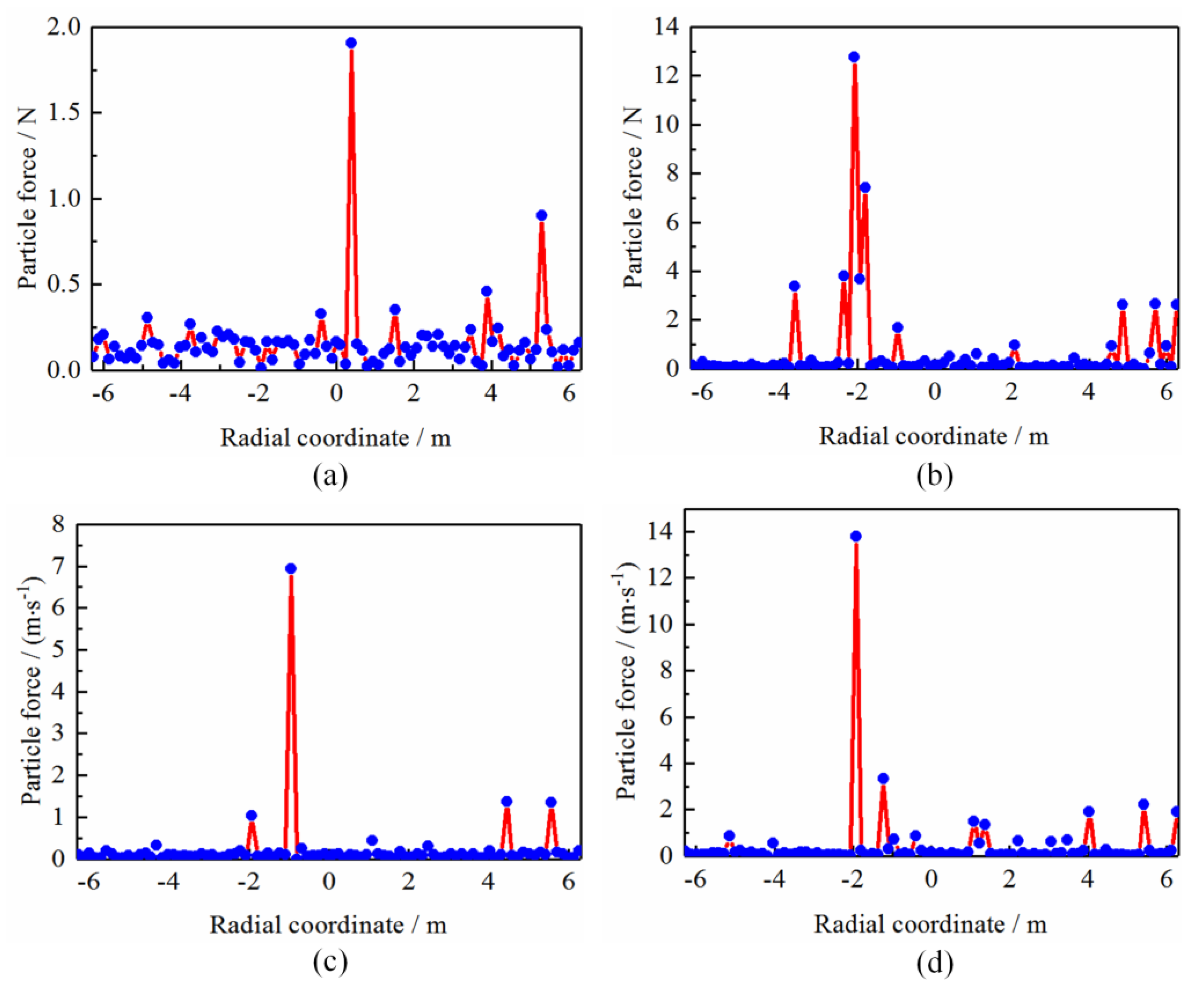
4.1. Particle Flow Distribution Characteristics

As mentioned above, gas–liquid–solid mixed flows are a complex turbulence course with high degree of disorder and are nonlinear. The flow properties of the particle volume fraction, speed, and turbulence energies are investigated to obtain the mass transfer properties.

Figure 4 describes the dynamic evolution process of a particle volume fraction. The inlet particles located at the top region flow into the mixing device. In Figure 4a, the particle distribution is uniform, and some particles are sucked up by the pipeline on the right. The particle volume fractions near the impeller components are small. In Figure 4b, particles at the top enter the container, and some particles gather in the lower impeller and the bottom of the right device. The particles at the top region are subjected to the rotating action of the upper impeller, and the wall hits some particles, as shown in Figure 4c. The volume fractions in the whole container are unequal, and some particles are deposited at the bottom. In Figure 4d, all particles enter the flow field, and many particles are attracted by the rotation effect of the lower impeller, resulting in a significantly higher volume fraction of particles on the left side than that on the right side. At this time, particles deposited at the bottom are suspended by the action of the central pipe blowing, which decreases the deposition of particles.

The volume fraction cloud diagrams of particles near the impellers are obtained to observe the particle distribution in the upper and lower impellers (Figure 5). Radial volume fraction distribution of particles in upper and lower impellers has similar characteristics. At the center, due to the rotating effect of the impeller, the particles at the edge of the impeller are thrown to the sides. The particle volume fractions are larger at impeller centers, their value is 0.016, and the particles have an aggregation phenomenon. Some particles are agglomerated on the right side of the lower impeller member, resulting in an increase in particle density at the radial coordinate of 3 m. The volume fraction of particles in other regions is relatively small. It shows particles can be distributed near the impeller center under the rotating effect.

4.2. Dynamic Evolution Laws of the Mixed Flow Field

The speed streamline diagrams are obtained to study mixing flow modes (Figure 6). The upper and lower impeller have symmetrical flow patterns in the initial state. The gas-filled pipe disturbs the particle phases, and the container takes on a nonlinear turbulence state under stirring speed and bottom blowing. In Figure 6b, the streamlines are subjected to the rotation influence, and particles are dispersed by the impeller, resulting in an apparent flow mode variation on both the left and right sides. There is a large velocity gradient in the center of the impeller. At this time, the flow mode of the lower impeller still maintains a balanced state, and the speed increases significantly. Many particles enter the flow field and greatly influence the flow pattern evolution of the entire flow field. An apparent local turbulent vortex is formed on the left side, increasing the randomness and complexity (Figure 6c). In Figure 6d, a large turbulent vortex formed on the container’s left side, causing many particles to flow to the lower impeller. The mixing process of turbulent vortices speeds up particle motions. The flow speed inside the pipeline is larger, which promotes particles to be sucked away by the pipeline.

The velocity distribution is the critical variable that reflects the characteristics of macroscopic flow. The velocity evolution cloud diagram of the mixed flow field inside the container is obtained (Figure 7). In Figure 7a, the gas-filling pipe rushes into the flow field, and its velocity is 8.0 m/s. Due to the lower impeller component’s large size and complex structure, the velocity near the impeller is larger and has a higher velocity gradient. In Figure 7b, the velocity cloud image on both sides of the lower impeller presents uniform characteristics and has large velocity values on both sides of the container wall. It is the effect of the joint action of the inflation and the lower impeller. Due to particle involvements in the upper impeller, speed values on the left side are larger. In Figure 7c, the flow field driven by the lower impeller has a higher flow speed, promoting the mixing process between vortices of different scales and improving mass transfer efficiency. In Figure 7d, the flow field under the combined action of the lower impeller and the upper impeller has high nonlinear turbulence characteristics. The velocity distribution is uneven, which makes the material mixing process more complicated.

To study the evolution characteristics of fluid velocity in the mixing space, the velocity evolution processes near impellers in the radial range of −6.3 m to 6.3 m in the mixing vessel when t = 7.0 s are selected (Figure 8). Figure 8a shows the characteristics of the total velocity evolution curve of the mixed flow field. The vessel wall velocity on the impeller section has the same value. In the range of radial coordinates −3~3 m, the velocities of upper and lower impellers increase significantly, and their peak values are 2.35 m·s⁻¹ and 2.75 m·s⁻¹, respectively. The flow field speeds of lower impellers decrease first and then increase, but the speeds of the upper impeller have the maximum value at the center z = 0. This indicates that the lower impeller consumes more energy to drive the fluid. In Figure 8b, the radial velocity of the lower impeller presents a characteristic called symmetry, but the speed differences near impellers are large. In Figure 8c, the upper and lower impellers have similar tangential velocity variation trends. The peak speed of the lower impeller is 2.25 m/s, and the peak speed of the upper impeller is 1.8 m/s. In Figure 8d, the axial velocity becomes complex and asymmetrical. The above phenomenon shows that gas causes a large disturbance to the flow patterns, and shear flows become complicated, which enhances turbulence and chaotic characteristics.

4.3. Energy Evolution Law of the Mixed Flow Field

The turbulence energy is the key characteristic of reflecting energy variation processes of turbulent vortices. Figure 9 describes the evolution processes of turbulent kinetic energy in smooth mixing. In Figure 9a, under the impeller rotating action and air inflation, the turbulence energies are concentrated at the bottom of the aeration pipe, and the peak value is 18.1 m²·s⁻². At this time, the turbulence energies are concentrated in the external measurement. In Figure 9b, the turbulence energies increase, and the turbulent kinetic energy near the wall has a larger value. In Figure 9c, the energy distributions on both sides of the mixing device are unbalanced, and the turbulence energies on the left side are more enormous. Due to the rotating effect of the lower impeller and the inflating action of the bottom, the local turbulent kinetic energy of the container wall continues to increase. However, the turbulence energies at the lower impeller form a low-value region. In Figure 9d, the turbulence energies reach the maximum value, which promotes the mixed transmission process of different fluid phases. The above phenomenon shows that bottom aeration can increase the nonlinearity of turbulence motions and improve mixing efficiencies between different scale vortices.

Based on the above, the dynamic evolution trend of the mixed flow field energies of upper and the lower impellers are obtained (Figure 10). Figure 10a shows the evolution characteristics of turbulence energies. The turbulent kinetic energy of the lower impeller is less minor than that of an upper impeller in the central region of the container, and the peak values are 0.082 m²·s⁻² and 0.185 m²·s⁻², respectively. The energy value increases first, then decreases, and then increases in the radial range of −3 m~3 m. It shows a large energy value at the edge of the impeller, and there is a low-value region in the middle of the impeller. Figure 10b shows the dynamic pressure pulsation trends. The dynamic pressures of the lower impeller are asymmetrical under the action of inflation interference, and the dynamic pressures at the center are slight. However, the upper impeller has the maximum pressure at the container center, with a peak value of 5300 Pa. In general, inflation greatly influences the energy variation process. It increases the mixed transmission process between the energy of vortex groups in the flow field of different scales.

4.4. Evolution Characteristics of Particle Flow Patterns

The evolution laws of particle velocity are acquired (Figure 11). The particle at the bottom has a larger speed value due to the aeration. In Figure 11a, the particles are subjected to gravity during the mixing process. The particle speed near the impeller varies, and the velocity gradient varies greatly. In Figure 11c,d, the particles at the bottom of the container move to the sides. Under the synergistic actions of the upper and lower impeller, many particles are involved in the external measurement of the impeller, which increases the complexity and randomness of the particle flow pattern. When the granular materials settle and the particle motions at the container bottom are hindered, the mixed effects will be decreased and the granular materials on the container wall will be challenging to stir more fully.

The particle velocity flow line of the mixed flow field is shown in Figure 12. The particle streamlines near the impeller are distorted. The particles at the bottom of the aerated pipe have the largest velocity with a peak velocity of 20.20 m/s. The particles at the bottom move to the container under the interference of inflation and then form a sizeable vortex structure. The particles at the top inlet continuously transport the mixed flow field and mix with the impeller rotation process, increasing the randomness of streamline patterns.

The velocity evolution curves in the section near the aerated pipe are obtained (Figure 13). The velocity size of the particles presents a uniform distribution, and its velocity fluctuates between 0.5 m/s and 2.8 m/s in Figure 13a. In Figure 13b, a large abrupt change in particle velocity occurs at the radial position of −1.8 m, and its peak value is 10.8 m/s. It shows that the turbulent randomness of the flow field is enhanced under the aeration effect, which increases the flow velocity of some particles. In Figure 13c, the abrupt peak value of particle velocity also appears at the radial position of −0.9 m. A similar phenomenon appears in Figure 13d. It shows that the turbulent motion is complex and nonlinear, and the velocity size of the particles has high randomness. The above phenomenon shows that a certain degree of aeration can improve material transport efficiency in mixed space.

The particle force curves are obtained in Figure 14. The particle has a mutation feature at the center of the container x = 0 m in Figure 14a, and the mutation peak value of the particle stress is 1.85 N. In Figure 14b, the particles are heavily stressed in the left −4~−2 m range and have multiple force pulse components. It shows that the turbulence nonlinearity of the left container is stronger than that of the right container, and the peak force is 13 N. In Figure 14c,d, the force on particles decreases slightly, and a few particles have a larger force. The above phenomenon shows that appropriate air volume can increase the turbulent transport course, improve particle suspension effects inside the container, and thus promote the material transport process between particle phases.

5. Conclusions

The material transport mechanisms and control strategy of gas–liquid–solid mixed flows have important scientific research significance for some engineering applications. We propose a CFD-DEM coupling modeling and solution approach to study mass transport mechanisms and flow patterns under inflation control. Aiming at the above objectives, relevant research work is carried out on the proposed modeling method, and the main conclusions are as follows:

(1)

A CFD-DEM coupling modeling method with porosity and soft models is presented to explore mass transport mechanisms and flow pattern evolution laws. Under the synergistic action of impeller rotating and inflation, the particle distribution in the mixing vessel is unequal. The particles in the upper and lower impellers have similar characteristics along the radial direction.

(2)

The mixed flow field presents highly nonlinear turbulent characteristics in the process of aerated disturbance and particle input. The macroscopic mixing process of turbulent vortices speeds up the material flow of the particle phase and promotes the mass transfer efficiency between different scale vortices. The velocity distribution is uneven, which makes the mixing process more complicated.

(3)

The turbulence energies are mainly concentrated in the inflation pipeline, and the energy peak values are 18.1 m²·s⁻². Due to the rotating effect of the lower impeller, the local energy near the vessel wall increases, and the low-energy areas are formed at the impeller center.

(4)

As particles settle and accumulate, particle movement is hindered, and the granular materials on the wall of the container are challenging to stir more fully. However, a certain degree of aeration can promote the particle suspension effect inside the container and improve the material transport efficiency inside the mixed space.

The gas–liquid–solid mixed flows are a complex turbulent mechanical problem, and the material transport mechanism and control strategy are important. Subsequent studies will explore facets of the lattice Boltzmann method and heat transport characteristics for gas–liquid–solid flows.

References

1. Jin, Z.; He, D.; Wei, Z. Intelligent fault diagnosis of train axle box bearing based on parameter optimization VMD and improved DBN. Eng. Appl. Artif. Intell. 2022, 110, 104713. [Google Scholar] [CrossRef]
2. Zheng, G.A.; Gu, Z.H.; Xu, W.X.; Li, Q.H.; Tan, Y.F.; Wang, C.Y.; Li, L. Gravitational surface vortex formation and suppression control: A review from hydrodynamic characteristics. Processes 2023, 11, 42. [Google Scholar] [CrossRef]
3. Xiao, Y.; Li, X.; Ren, S. Hydrodynamics of gas phase under typical industrial gassing rates in a gas-liquid stirred tank using intrusive image-based method. Chem. Eng. Sci. 2020, 227, 115923. [Google Scholar] [CrossRef]
4. Delafosse, A.; Morchain, J.; Guiraud, P. Trailing vortices generated by a Rushton turbine: Assessment of URANS and large Eddy simulations. Chem. Eng. Res. Des. 2009, 87, 401–411. [Google Scholar] [CrossRef]
5. Li, L.; Xu, W.X.; Tan, Y.F.; Yang, Y.S.; Yang, J.G.; Tan, D.P. Fluid-induced vibration evolution mechanism of multiphase free sink vortex and the multi-source vibration sensing method. Mech. Syst. Signal Process 2023, 189, 110058. [Google Scholar] [CrossRef]
6. Coelho, R.C.V.; Araujo, N.A.M.; da Gama, M.M.T. Dispersion of activity at an active-passive nematic interface. Soft. Matter 2022, 18, 7642–7653. [Google Scholar] [CrossRef]
7. Sedahamed, M.; Coelho, R.C.V.; Araujo, N.A.M.; Wahba, E.M.; Warda, H.A. Study of fluid displacement in three-dimensional porous media with an improved multicomponent pseudopotential lattice Boltzmann method. Phys. Fluids 2023, 34, 103303. [Google Scholar] [CrossRef]
8. Li, L.; Tan, Y.F.; Xu, W.X.; Ni, Y.S.; Yang, J.G.; Tan, D.P. Fluid-induced transport dynamics and vibration patterns of multiphase vortex in the critical transition states. Int. J. Mech. Sci. 2023, 252, 108376. [Google Scholar] [CrossRef]
9. Su, R.A.; Gao, Z.Y.; Chen, Y.Y.; Zhang, C.Q. Large-eddy simulation of the influence of hairpin vortex on pressure coefficient of an operating horizontal axis wind turbine. Energy Convers. Manag. 2022, 267, 115864. [Google Scholar] [CrossRef]
10. Zhang, L.; Yuan, Z.; Tan, D. An improved abrasive flow processing method for complex geometric surfaces of titanium alloy artificial joints. Appl. Sci. 2018, 8, 1037. [Google Scholar] [CrossRef]
11. Li, L.; Lu, B.; Xu, W.X.; Gu, Z.H.; Yang, Y.S.; Tan, D.P. Mechanism of multiphase coupling transport evolution of free sink vortex. Acta Phys. Sin. 2023, 72, 034702. [Google Scholar] [CrossRef]
12. Yin, Z.C.; Lu, J.F.; Li, L.; Wang, T.; Wang, R.H.; Fan, X.H.; Lin, H.K.; Huang, Y.S.; Tan, D.P. Optimized Scheme for Accelerating the Slagging Reaction and Slag-Metal-Gas Emulsification in a Basic Oxygen Furnace. Appl. Sci. 2020, 10, 5101. [Google Scholar] [CrossRef]
13. Kan, K.; Xu, Y.H.; Li, Z.X.; Xu, H.; Chen, H.X.; Zi, D. Numerical study of instability mechanism in the air-core vortex formation process. Eng. Appl. Comput. Fluid Mech. 2023, 17, 2156926. [Google Scholar] [CrossRef]
14. Li, L.; Gu, Z.H.; Xu, W.X.; Tan, Y.F.; Fan, X.H.; Tan, D.P. Mixing mass transfer mechanism and dynamic control of gas-liquid-solid multiphase flow based on VOF-DEM coupling. Energy 2023, 272, 127015. [Google Scholar] [CrossRef]
15. Che, H.Q.; Werner, D.; Seville, J. Evaluation of coarse-grained CFD-DEM models with the validation of PEPT measurement. Particuology 2023, 82, 48–63. [Google Scholar] [CrossRef]
16. Li, L.; Li, Q.H.; Ni, Y.S.; Wang, C.Y.; Tan, Y.F.; Tan, D.P. Critical penetrating vibration evolution behaviors of the gas-liquid coupled vortex flow. Energy 2023, in press.
17. Delacroix, B.; Rastoueix, J.; Fradette, L. CFD-DEM simulations of solid-liquid flow in stirred tanks using a non-inertial frame of reference. Chem. Eng. Sci. 2021, 230, 116137. [Google Scholar] [CrossRef]
18. Ting, S.; Yinyu, H.U.; Wentan, W.; Yong, J.; Cheng, Y. Simulation of solid suspension in a stirred tank using CFD-DEM coupled approach. Chin. J. Chem. Eng. 2013, 21, 1069–1081. [Google Scholar]
19. Blais, B.; Lassaigne, M.; Goniva, C.; Fradette, L.; Bertrand, F. Development of an unresolved CFD-DEM model for the flow of viscous suspensions and its application to solid-liquid mixing. J. Comput. Phys. 2016, 318, 201–221. [Google Scholar] [CrossRef]
20. Blais, B.; Bertrand, O.; Fradette, L.; Bertrand, F. CFD-DEM simulations of early turbulent solid-liquid mixing: Prediction of suspension curve and just-suspended speed. Chem. Eng. Res. Des. 2017, 123, 388–406. [Google Scholar] [CrossRef]
21. Sun, X.; Sakai, M. Three-dimensional simulation of gas-solid-liquid flows using the DEM-VOF method. Chem. Eng. Sci. 2015, 134, 531–548. [Google Scholar] [CrossRef]
22. Kang, Q.; He, D.; Zhao, N.l. Hydrodynamics in unbaffled liquid-solid stirred tanks with free surface studied by DEM-VOF method. Chem. Eng. J. 2020, 386, 122846. [Google Scholar] [CrossRef]
23. Zheng, G.A.; Shi, J.L.; Li, L.; Li, Q.H.; Gu, Z.H.; Xu, W.X.; Lu, B. Fluid-solid coupling-based vibration generation mechanism of the multiphase vortex. Processes 2023, 11, 568. [Google Scholar] [CrossRef]
24. Li, C.J.; Zou, Y.Q.; Li, G.Y. Hydrodynamic characteristics of pyrolyzing biomass particles in a multi-chamber fluidized bed. Powder Technol. 2023, 421, 118403. [Google Scholar] [CrossRef]
25. Boyer, C.; Duquenne, A.M.; Wild, G. Measuring techniques in gas-liquid and gas-liquid-solid reactors. Chem. Eng. Sci. 2002, 57, 3185–3215. [Google Scholar] [CrossRef]
26. Lee, B.W.; Dudukovic, M.P. Determination of flow regime and gas holdup in gas-liquid stirred tanks. Chem. Eng. Sci. 2014, 109, 264–275. [Google Scholar] [CrossRef]
27. Gu, Y.H.; Zheng, G.A. Dynamic Evolution Characteristics of the Gear Meshing Lubrication for Vehicle Transmission System. Processes 2023, 11, 561. [Google Scholar] [CrossRef]
28. Li, L.; Yang, Y.S.; Xu, W.X.; Lu, B.; Gu, Z.H.; Yang, J.G.; Tan, D.P. Advances in the multiphase vortex-induced vibration detection method and its vital technology for sustainable industrial production. Appl. Sci. 2022, 12, 8538. [Google Scholar] [CrossRef]
29. Yu, J.H.; Wang, S.; Kong, D.L. Coal-fueled chemical looping gasification: A CFD-DEM study. Fuel 2023, 345, 128119. [Google Scholar] [CrossRef]
30. Fontaine, A.; Guntzburger, Y.; Bertrand, F.; Fradette, L.; Heuzey, M.C. Experimental investigation of the flow dynamics of rheologically complex fluids in a Maxblend impeller system using PIV. Chem. Eng. Res. Des. 2013, 91, 7–17. [Google Scholar] [CrossRef]
31. Montante, G.; Paglianti, A. Gas hold-up distribution and mixing time in gas-liquid stirred tanks. Chem. Eng. J. 2015, 279, 648–658. [Google Scholar] [CrossRef]
32. Kumar, S.S.; Delauré, Y.M.C. An assessment of suitability of a simple vof/plic-csf multiphase flow model for rising bubble dynamics. J. Comput. Multiph. Flows 2012, 4, 65–83. [Google Scholar] [CrossRef]
33. Wang, H.; Wang, X.Y.R.; Wu, Y.P. Study of CFD-DEM on the Impact of the Rolling Friction Coefficient on Deposition of Lignin Particles in a Single Ceramic Membrane Pore. Membranes 2023, 123, 382. [Google Scholar] [CrossRef]
34. Wang, Y.; Ni, P.; Wen, D. Dynamic performance optimization of circular sawing machine gearbox. Appl. Sci. 2019, 9, 4458. [Google Scholar] [CrossRef]
35. Tamburini, A.; Cipollina, A.; Micale, G.; Brucato, A.; Ciofalo, M. CFD simulations of dense solid-liquid suspensions in baffled stirred tanks: Prediction of the minimum impeller speed for complete suspension. Chem. Eng. J. 2012, 193, 234–255. [Google Scholar] [CrossRef]
36. Wang, J.J.; Han, Y.; Gu, X.P. Effect of agitation on the fluidization behavior of a gas-solid fluidized bed with a frame impeller. AIChE J. 2013, 59, 1066–1074. [Google Scholar] [CrossRef]
37. Li, L.; Lu, J.F.; Fang, H.; Yin, Z.C.; Wang, T.; Wang, R.H.; Fan, X.H.; Zhao, L.J.; Tan, D.P.; Wan, Y.H. Lattice Boltzmann method for fluid-thermal systems: Status, hotspots, trends and outlook. IEEE Access 2020, 8, 27649–27675. [Google Scholar] [CrossRef]
38. Li, Q.; Xiang, P.; Li, L. Phosphorus mining activities alter endophytic bacterial communities and metabolic functions of surrounding vegetables and crops. Plant Soil. 2023, 227. [Google Scholar] [CrossRef]
39. Xie, L.; Luo, Z.H. Modeling and simulation of the influences of particle-particle interactions on dense solid-liquid suspensions in stirred vessels. Chem. Eng. Sci. 2018, 176, 439–453. [Google Scholar] [CrossRef]
40. Li, L.; Tan, D.P.; Yin, Z.C.; Wang, T.; Fan, X.H.; Wang, R.H. Investigation on the multiphase vortex and its fluid-solid vibration characters for sustainability production. Renew. Energy 2021, 175, 887–909. [Google Scholar] [CrossRef]
41. Jovanović, A.; Pezo, M.; Pezo, L.; Lević, L. DEM/CFD analysis of granular flow in static mixers. Powder Technol. 2014, 266, 240–248. [Google Scholar] [CrossRef]
42. Liu, S.; Lu, Y.; Li, J. A blockchain-based interactive approach between digital twin-based manufacturing systems. Comput. Ind. Eng. 2023, 175, 108827. [Google Scholar] [CrossRef]
43. Li, L.; Qi, H.; Yin, Z.C.; Li, D.F.; Zhu, Z.L.; Tangwarodomnukun, V.; Tan, D.P. Investigation on the multiphase sink vortex Ekman pumping effects by CFD-DEM coupling method. Powder Technol. 2020, 360, 462–480. [Google Scholar] [CrossRef]
44. Wang, S.; Shen, Y.S. CFD-DEM-VOF-phase diagram modelling of multi-phase flow with phase changes. Chem. Eng. Sci. 2023, 273, 118652. [Google Scholar] [CrossRef]
45. Chen, J.C.; Han, P.C.; Zhang, Y.; You, T.; Zheng, P.Y. Scheduling energy consumption-constrained workflows in heterogeneous multi-processor embedded systems. J. Syst. Archit. 2023, 142, 102938. [Google Scholar] [CrossRef]
46. Li, L.; Tan, D.P.; Wang, T.; Yin, Z.C.; Fan, X.H.; Wang, R.H. Multiphase coupling mechanism of free surface vortex and the vibration-based sensing method. Energy 2021, 216, 119136. [Google Scholar] [CrossRef]
47. Wang, T.; Wang, C.Y.; Yin, Y.X.; Zhang, Y.K.; Li, L.; Tan, D.P. Analytical approach for nonlinear vibration response of the thin cylindrical shell with a straight crack. Nonlinear Dyn. 2023, 111, 10957–10980. [Google Scholar] [CrossRef]
48. Wu, L.; Gong, M.; Wang, J. Development of a DEM-VOF model for the turbulent free-surface flows with particles and its application to stirred mixing system. Ind. Eng. Chem. Res. 2018, 57, 1714–1725. [Google Scholar] [CrossRef]
Figure 1. VOF-DEM computer flow chart.
Processes 11 02254 g001
Figure 2. Diagram of hybrid space structure.
Processes 11 02254 g002
Figure 3. Grids division of the numerical model.
Processes 11 02254 g003
Figure 4. Cloud diagrams of particle volume fraction in the mixed flow field. (a) t = 1.0 s. (b) t = 4.0 s. (c) t = 7.0 s. (d) t = 10.0 s.
Processes 11 02254 g004
Figure 5. Particle volume fractions of upper and lower impellers.
Processes 11 02254 g005
Figure 6. Streamline cloud diagram at the cross-section. (a) t = 1.0 s. (b) t = 4.0 s. (c) t = 7.0 s. (d) t = 10.0 s.
Processes 11 02254 g006
Figure 7. Velocity cloud diagram at the cross-section. (a) t = 1.0 s. (b) t = 4.0 s. (c) t = 7.0 s. (d) t = 10.0 s.
Processes 11 02254 g007
Figure 8. Velocity variation curves of the upper and lower impellers. (a) Total velocity. (b) Radial velocity. (c) Tangential velocity. (d) Axial velocity.
Processes 11 02254 g008
Figure 9. Cloud diagrams of the turbulence energy. (a) t = 1.0 s. (b) t = 4.0 s. (c) t = 7.0 s. (d) t = 10.0 s.
Processes 11 02254 g009
Figure 10. Energy evolution trend of the mixed flow field. (a) Turbulent kinetic energy. (b) Dynamic pressure.
Processes 11 02254 g010
Figure 11. Particle velocity cloud diagrams at the cross-section. (a) t = 1.0 s. (b) t = 4.0 s. (c) t = 7.0 s. (d) t = 10.0 s.
Processes 11 02254 g011
Figure 12. Particle velocity streamlines at the cross-section. (a) t = 1.0 s. (b) t = 4.0 s. (c) t = 7.0 s. (d) t = 10.0 s.
Processes 11 02254 g012
Figure 13. Particle velocity variation curves. (a) t = 1.0 s. (b) t = 4.0 s. (c) t = 7.0 s. (d) t = 10.0 s.
Processes 11 02254 g013
Figure 14. Particle force variation curves. (a) t = 1.0 s. (b) t = 4.0 s. (c) t = 7.0 s. (d) t = 10.0 s.
Processes 11 02254 g014