A New Integrated Model for Simulating Adaptive Cycle Engine Performance Considering Variations in Tip Clearance

Abstract

The low-fidelity simulation method cannot meet the requirements for predicting the performance of an adaptive cycle engine (ACE), especially when considering tip clearance variations in the compression and expansion systems. The tip clearances of the components of an ACE, such as the adaptive fan and turbine, vary drastically under different operating conditions. Though the tip clearance significantly impacts the engine’s performance, including its thrust and fuel consumption, variations in tip clearance are not considered in traditional ACE simulation models. This paper developed a new integrated model for predicting ACE performance, including multi-fidelity simulation models of the components and a newly developed, simplified model for predicting tip clearance. Specifically, the integrated model consists of a zero-dimensional (0D) engine performance simulation model, a three-dimensional (3D) adaptive fan numerical simulation model, a one-dimensional (1D) low-pressure-turbine (LPT) mean line model, and a multi-dimensional (MD) tip clearance prediction model. The integrated model solved the problem of considering the impact of tip clearance on an ACE and further improved the accuracy of thrust and fuel consumption predictions. Specifically, considering variations in the tip clearances under the design conditions, the differences in the thrust and specific fuel consumption (SFC) of the ACE are 1% and 0.3%, respectively. In conclusion, the integrated model provides a useful tool for evaluating the performance of an ACE while considering tip clearance variations.

1. Introduction

An adaptive cycle engine (ACE) aims to balance its thrust and fuel consumption by introducing wide-range variable-geometry mechanisms, and it is considered an advanced propulsion system for the next generation [1]. However, the operating modes and control schemes of an ACE are more complex than those of conventional engines, resulting in a more challenging process for predicting the performance of an ACE. Generally, conventional engines adopt a low-fidelity zero-dimensional (0D) simulation method based on generic characteristic maps of their components to predict performance. However, the design and analysis requirements of an ACE cause difficulty for the 0D method. The multi-fidelity simulation methods proposed by Claus [2] and Alexiou [3] are promising tools for predicting the performance of an ACE. Specifically, these methods can be classified as de-coupled, iteratively coupled, and fully coupled, depending on the coupling tightness level, which balances the computing time and accuracy. High-fidelity component models were widely researched, including the one-dimensional (1D) model studied by Kim [4], Follen [5], and Kolias [6] and the three-dimensional (3D) model by Pilet [7] and Klein [8]. In addition to the conventional components, high-fidelity simulation methods are also used for ACE components, such as the front variable area bypass injector (FVABI), which can be simulated via de-coupled [9] and fully-coupled [10] methods. However, there are fewer studies on integrating high-fidelity models of other critical components, such as the adaptive fan and variable-geometry turbine, into the 0D ACE model, which needs more attention for the ACE design, especially when considering the variations in tip clearance.

The tip clearances of the engine components significantly impact the performance of each component, thus affecting the engine’s performance. Ameri et al. [11] found that turbine efficiency decreased by about 4.5% when the tip clearance increased from 0% to 3% of the blade height. Bringhenti and Barbosa [12] studied the effects of tip clearance on a turbojet engine and found that an increased clearance would cause a deterioration in the engine’s performance. Though much research has been conducted on traditional engines, the impact of variations in tip clearance on the ACE is still unclear and needs to be clarified. Variations in tip clearance are mainly caused by thermal and centrifugal force loads [13]. A numerical simulation can obtain more accurate results, but the calculation process is complicated and consumes a significant amount of time [14,15,16]. For example, using the 3D fluid–solid thermal coupling method (FSTM), it takes a 40-core processor approximately 18,000 min to finish the simulation of the tip clearance variation process of a single-stage turbine, which lasts for a thousand seconds [17]. On the other hand, a simplified model is usually necessary for conducting an analysis in the early stage of engine design, though the prediction accuracy is limited due to the model’s simplicity. More specifically, the traditional simplified model is usually built by considering the deformation of the shroud, blade, and disk along the 1D direction after simplifying the geometry and boundary conditions [18,19,20,21,22]. Furthermore, the models cannot consider the spatial effects, including variations in the thicknesses of the blade and disk, and the radial heat transfer of the disk. However, Dong [23] and Luberti [24] found that the growth caused by the radial temperature distribution of the disk cannot be ignored and affects the tip clearance significantly. Meanwhile, variations in the thicknesses of the blade and disk cannot be ignored [25,26]. Therefore, a new multi-dimensional (MD) tip clearance prediction model was established based on the radial heat transfer characteristics of the disk and the variable cross-section characteristics of the components. Moreover, the accuracy of the model was validated via the 3D FSTM.

In this work, the integrated model consists of a 0D engine performance simulation model, a 3D adaptive fan numerical simulation model, a 1D low-pressure-turbine (LPT) mean line model, and an MD tip clearance prediction model. The 0D engine model was established on the MATLAB and Simulink simulation platforms. The MD tip clearance model, established on the MATLAB platform, was applied to the components on the low-pressure spool of an ACE. The tip clearances of the adaptive fan and the LPT were predicted based on the boundary conditions from the 0D engine model. Meanwhile, a characteristic map of the adaptive fan was predicted by the 3D model on the ANSYS CFX19.2 platform, and the de-coupled method was used to map changes when the tip clearance changed. Furthermore, the performance of the LPT was predicted by the 1D mean line model on the MATLAB simulation platform, and the iteratively coupled method was used to predict variations in performance with variations in the tip clearance. Finally, variations in the performances of the ACE were predicted via the integrated model. By comparing the ACE’s performance with the assembled clearance and its performance with the predicted clearance, it is shown that variations in tip clearance cannot be ignored during the operation of the engine, and the effectiveness of the method is also proved.

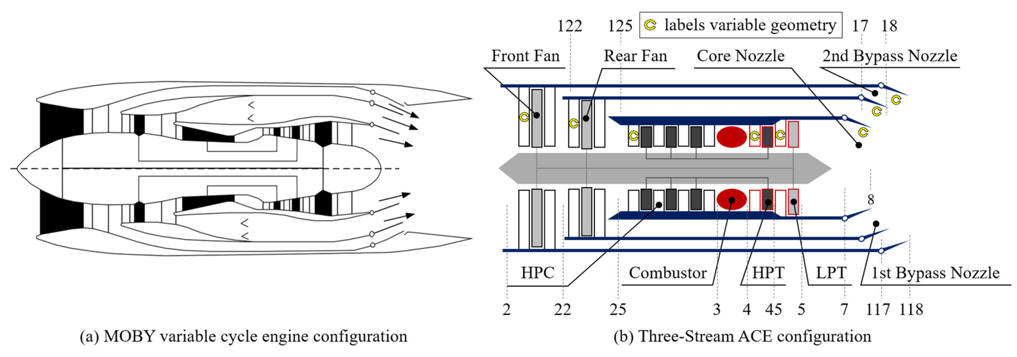
2. Case Description

The research object of this paper is an ACE with a three-stream configuration, as shown in Figure 1b. This ACE was derived from a modulating bypass (MOBY) variable-cycle engine [27], as shown in Figure 1a, and the three-spool configuration of the MOBY was replaced by a two-spool configuration. The ACE consisted of an adaptive fan, including front and rear fans, a high-pressure compressor (HPC), a combustor, a high-pressure turbine (HPT), an LPT, a core nozzle, a first-bypass nozzle, and a second-bypass nozzle, rather than a variable-area bypass injector (VABI). The adjustable components included guide vanes or stator vanes on the front and rear fans, the HPC, HPT, LPT, and three nozzles.

The design operating point of the ACE was set to be at sea level and static state, and the main parameters considered at this point are shown in

Table 1. Design operating point parameters.

Parameter	Value	Unit
Front fan pressure ratio	1.8	-
Rear fan pressure ratio	1.42	-
HPC pressure ratio	7.0	-
Turbine inlet temperature (T4)	1700	K
Front fan bypass ratio	0.15	-
Rear fan bypass ratio	1.0	-
Specific thrust	543	N·s/kg
Specific fuel consumption (SFC)	70.68	kg/(kN·h)

. The front fan bypass ratio is equal to the ratio of the mass flow rate in the second bypass duct to the mass flow rate in the rear fan. The rear fan bypass ratio is equal to the ratio of the mass flow rate in the first bypass duct to the mass flow rate in the HPC. The front and rear fans and the LPT all consist of a single stage with rotors and stators, while the front fan consists of an inlet guide vane (IGV), a rotor, and a stator. The geometrical parameters of the adaptive fan and the LPT were designed according to the performance of each component and are shown in

Table 2. Geometrical parameters of the adaptive fan and LPT.

Parameter	Value	Unit
Number of S0 (front fan IGV) blades	15	-
Number of R1 (front fan rotor) blades	28	-
Number of S1 (front fan stator) blades	46	-
Assembled tip clearance of the front fan	0.3	mm
Number of rear fan rotor blades	29	-
Number of rear fan stator blades	49	-
Assembled tip clearance of the rear fan	0.3	mm
Number of LPT stator blades	36
Number of LPT rotor blades	53
Assembled tip clearance of the LPT	0.3	mm

.

3. Methodology

This section establishes the ACE integrated model, including the 0D engine performance simulation model, the 3D adaptive fan numerical simulation model, the 1D LPT mean line model, and the MD tip clearance prediction model. The 0D engine performance simulation model provides the engine performance and boundary conditions for the other models. The 3D numerical simulation and 1D mean line models provide the adaptive fan and LPT performance, respectively. The MD tip clearance prediction model provides variations in the tip clearance under different rotating speeds. Finally, the engine performance considering tip clearance variations can be obtained.

3.1. ACE Performance Simulation Method

3.1.1. Zero-Dimensional Engine Performance Simulation Model

The 0D engine performance simulation model was developed on the MATLAB and Simulink platforms based on the object-oriented programming technique, adopting the open-source package T-MATS (toolbox for the modeling and analysis of thermodynamic systems) [28]. The empirical relations from Refs. [29,30] were used for the HPC, HPT, and LPT, adding the impacts of variable geometry on the components’ characteristics. Furthermore, variable multi-angle characteristic maps were used for the front and rear fans, which reflect characteristics including the mass flow rate, pressure ratio, and isentropic efficiency under different guide vane angles. The iteration and error variables of the engine required to reach equation convergence are shown in

Table 3. Off-design point iteration and error variables.

Component Class	Class Number	Iteration Variable	Error Variable
Inlet	1	Mass flow	-
Compressor	3	R-value	Mass flow
Splitter	2	Split ratio	-
Burner	1	Fuel air ratio	-
Turbine	2	Expansion ratio	Mass flow
Nozzle	3	-	Mass flow
Shaft	2	Spool speed	Power
Summary	14	11	10

, which is based on the matching of each component at the off-design point. Moreover, after setting the low-pressure spool speed, the Newton–Raphson iterative method was adopted to evaluate the off-design point performance.

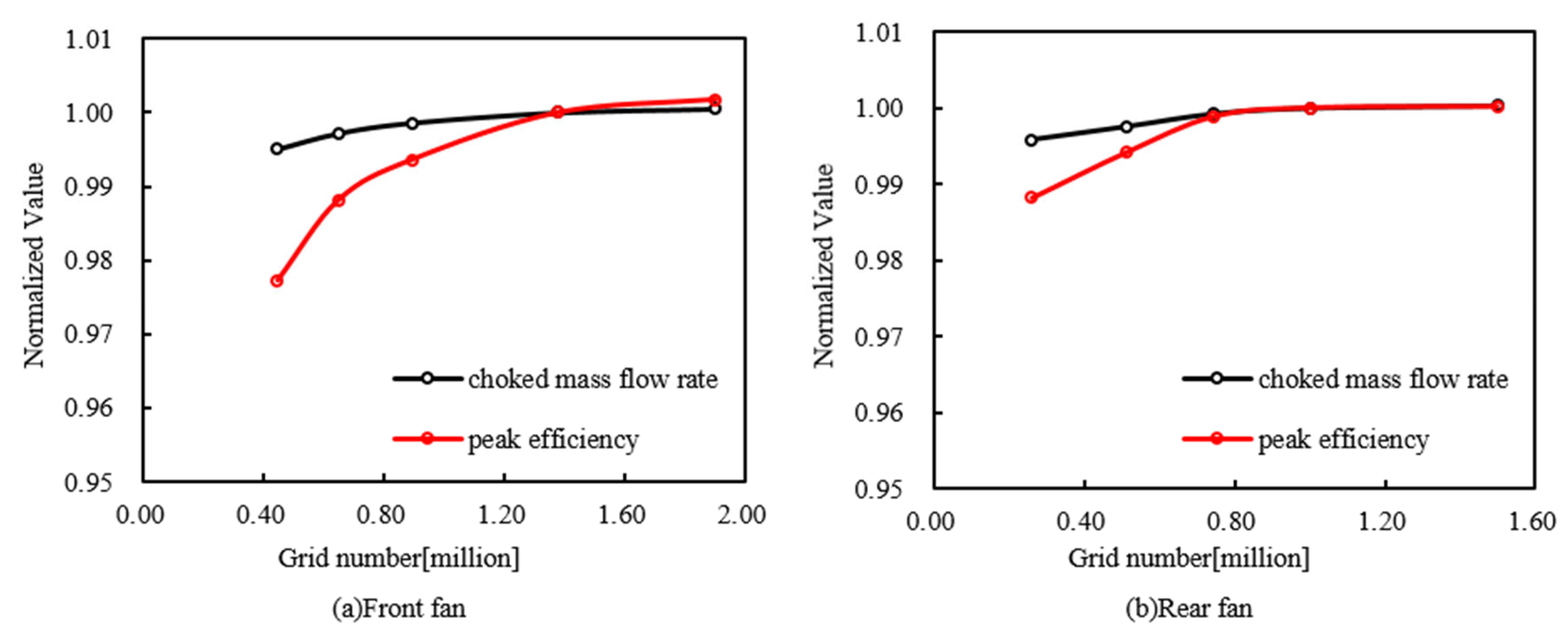
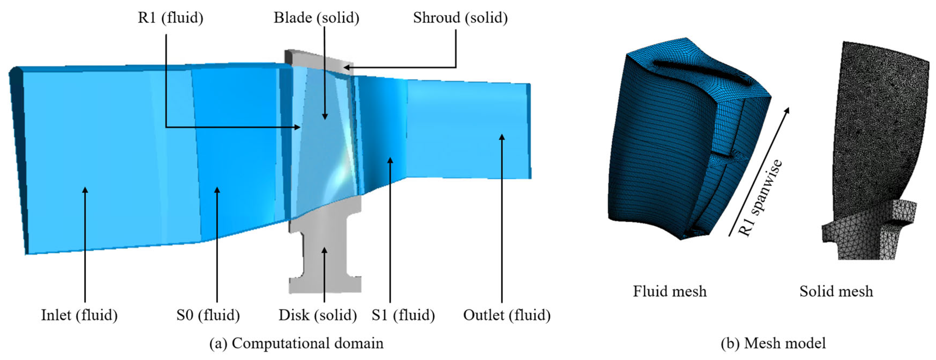
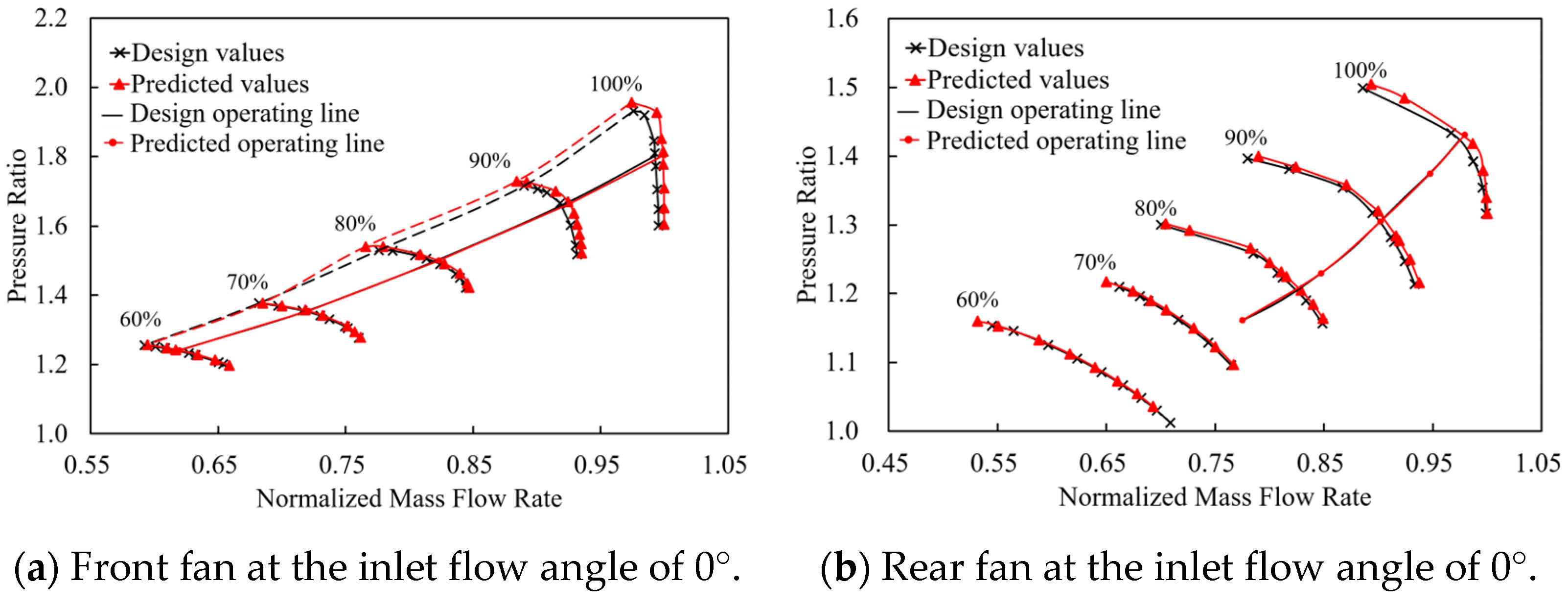
3.1.2. Three-Dimensional Adaptive Fan Numerical Simulation Model

ANSYS CFX19.2 was adopted for the 3D numerical simulation of the characteristic map of the adaptive fan. It adopted the second-order-accuracy high-resolution method and second-order Euler backward scheme for spatial and temporal discretization, respectively. Moreover, the shear stress transport (SST) model was adopted for the turbulence closure, and the mixing-plane model was used for the rotor–stator interface. Furthermore, considering the cyclic symmetric structure of the adaptive fan, a single-passage setting was adopted for both the front and rear fans. Moreover, TurboGrid was used to generate the mesh, and the passage and tip areas were meshed as an H-grid, while the blade area was meshed as an O-grid. Furthermore, the grid numbers of the front and rear fans were 1.37 million and 1 million, respectively. More specifically, the computational domain and the mesh of the front fan are shown in Figure 2, and those of the rear fan are similar.

The mesh independence was studied prior to numerous simulations. Five types of mesh from the front and rear fans were investigated, respectively. The calculated parameters are plotted in Figure 3, including the normalized choked mass flow rate and peak efficiency. It can be concluded that the CFD simulation remains unchangeable after the mesh nodes reach 1.3 million for the front fan and 1.0 million for the rear fan. Hence, the adopted mesh is appropriate for this research.

3.1.3. One-Dimensional LPT Mean Line Model

The 1D LPT mean line model was developed on the MATLAB platform in Ref. [31]. The off-design profile loss model is shown in Equation (1), and the empirical coefficients were optimized based on Kacker and Okapuu [32]. The deviation model is shown in Equation (2), the empirical coefficients of which were optimized from Zhu’s research [33]. In Equation (1), ω, ω_ref, i, and i_stall are the profile loss coefficient, the profile loss coefficient of the reference value, the incidence angle, and the stalling incidence angle, respectively. In Equation (2), δ, γ, c, β₁, β_1m, β_2m, t_max, and Re are the deviation angle, stagger angle, chord length, inlet flow angle, inlet metal angle, outlet metal angle, maximum blade thickness, and Reynolds number, respectively.

$$\omega =\left[0.2235{\left(i/i_{\mathrm{stall}}\right)}^3+1.4057{\left(i/i_{\mathrm{stall}}\right)}^2+0.4796\left(i/i_{\mathrm{stall}}\right)+1.0\right]{\omega }_{\mathrm{ref}}$$

(1)

$$\delta =12.5\frac{{\left(\gamma /c\right)}^{0.05}{\left({\beta }_1+{\beta }_{2\mathrm{m}}\right)}^{0.63}{\cos }^2(\gamma ){\left(t_{\max }/c\right)}^{0.29}}{\left(32.3+0.01{\beta }_{1\mathrm{m}}^{2.07}\right){\tanh }^{0.2}(\mathrm{Re}/200000)}$$

(2)

Also, the influence of turbine tip clearance proposed by Kacker and Okapuu [32,34] was considered, as shown in Equation (3). In Equation (3), ${\mathrm{\gamma }}_{cl}$, B, Z, c, H, and t_cl are the clearance loss coefficient, the constant defined by the Kacker–Okapuu loss system, the Ainley–Mathieson loading parameter, the chord length, the blade height, and the tip clearance, respectively.

$${\mathrm{\gamma }}_{\mathrm{cl}}=B\times Z\times \left(\frac{c}{H}\right)\times {\left(\frac{t_{\mathrm{cl}}}{H}\right)}^{0.78}$$

(3)

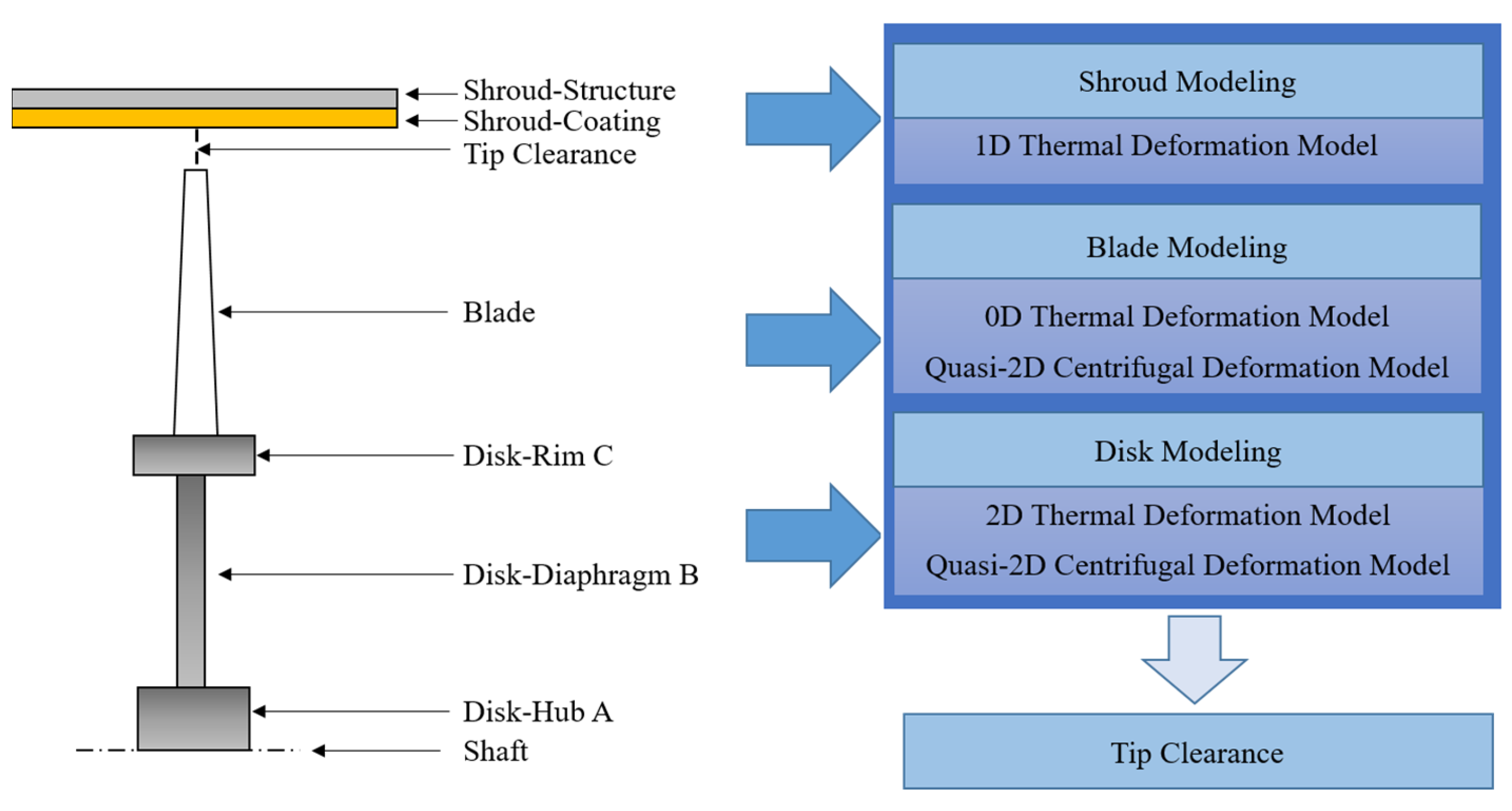
3.2. MD Tip Clearance Prediction Model

This section established an MD tip clearance prediction model with three components, the shroud, blade, and disk, which was developed in the MATLAB platform. Furthermore, considering the geometries and heat transfer characteristics of the different components, a 0D–2D coupled prediction model was established for each component, as shown in Figure 4. The tip clearance prediction model was first established for transient tip clearance predictions [17]. However, it can also be used for steady-state predictions, and the equation for clearance is as follows:

$$TC=T{C}_{\mathrm{assemble}}+(u_{\mathrm{shroud}}-u_{\mathrm{blade}}-u_{\mathrm{disk}})$$

(4)

where $TC$ is the predicted tip clearance, $T{C}_{\mathrm{assemble}}$ is the assembled tip clearance, and $u_{\mathrm{shroud}}$, $u_{\mathrm{blade}}$, and $u_{\mathrm{disk}}$ represent the deformations of the shroud, blade, and disk, respectively. Furthermore, the following are the deformation models of each component.

3.2.1. Shroud Modeling

The radial deformation of the shroud is mainly caused by thermal loads. Moreover, the 1D thermal deformation model of the shroud was established based on the 1D difference method [21] and the elastic theory [26]. Furthermore, the shroud is usually divided into an abradable coating and a superalloy structure, as shown in Figure 4. The temperatures of the two layers were calculated via 1D difference equations; interested readers may refer to Ref. [17]. In addition, the model adopts the flat plate heat transfer formula from Ref. [35] for the heat transfer coefficient of the outer wall of the shroud and the empirical formula from Ref. [36] for the heat transfer coefficient of the inner wall of the shroud. The shroud can be considered a hollow cylinder, and the thermal deformation of the shroud can be calculated based on the elastic theory. The deformations of the inner and outer walls of each layer can be derived, respectively. Furthermore, the radial deformation compatibility and force equilibrium were considered at the interface of the two layers. The thermal deformation of the shroud $u_{\mathrm{shroud}\_\mathrm{thermal}}$ can be calculated by combing and solving the inner and outer wall equations of each layer.

3.2.2. Blade Modeling

The radial deformation of the blade is mainly caused by thermal and centrifugal loads. The 0D thermal deformation and the quasi-2D centrifugal deformation model of the blade were established based on the lumped capacitance method and the elastic theory, respectively. After using the lumped capacitance method, the temperature of the blade at each time step p can be calculated using the following equation [21]:

$$T_{\mathrm{blade}}^{p+1}=(T_{\mathrm{blade}}^p-T_{\mathrm{ref}}^p)\times e^{-\frac{\mathrm{\Delta }t}{{\tau }^p}}+T_{\mathrm{ref}}^p$$

(5)

where $T_{\mathrm{blade}}^{p+1}$, $T_{\mathrm{blade}}^p$, $T_{\mathrm{ref}}^p$, $\tau$, and $\mathrm{\Delta }t$ are the temperature of the blade at time step p + 1, the temperature of the blade at time step p, the reference temperature at time step p, the time constant, and the time interval of each time step, respectively. For a blade without cooling, the reference temperature $T_{\mathrm{ref}}^p$ is equal to the temperature of the main flow $T_{\mathrm{f}}^p$, while for a blade with cooling, it can be defined as follows:

$$T_{\mathrm{ref}}^p=\eta \times (T_{\mathrm{cool}}^p-T_{\mathrm{f}}^p)+T_{\mathrm{f}}^p$$

(6)

where $T_{\mathrm{cool}}^p$ is the temperature of the cooling air and $\eta$ is the film cooling efficiency. When the temperature of the blade becomes steady, the model of the blade’s thermal deformation can be calculated as follows:

$$u_{\mathrm{blade}\_\mathrm{thermal}}={\alpha }_{\mathrm{blade}}\times L_{\mathrm{blade}}\times T_{\mathrm{blade}}$$

(7)

where $u_{\mathrm{blade}\_\mathrm{thermal}}$, ${\alpha }_{\mathrm{blade}}$, $L_{\mathrm{blade}}$, and $T_{\mathrm{blade}}$ are the thermal deformation, the thermal expansion coefficient, the length of the blade, and the temperature of the blade, respectively. A quasi-2D centrifugal deformation model was established to analyze the centrifugal deformation of the variable-thickness blade. The centrifugal deformation equation of the blade was derived as follows:

$$u_{\mathrm{blade}\_\mathrm{centrifugal}}=\frac{{\rho }_{\mathrm{blade}}{L}_{{}_{\mathrm{blade}}}^2}{2E_{\mathrm{blade}}}{\left(\frac{2\pi }{60}N\right)}^2\left[\left(1-\frac{2}{3}a\right)r_{\mathrm{disk}}+\left(\frac{2}{3}-\frac{1}{2}a\right)L_{\mathrm{blade}}\right]$$

(8)

where $u_{\mathrm{blade}\_\mathrm{centrifugal}}$, ${\rho }_{\mathrm{blade}}$, $E_{\mathrm{blade}}$, a, $r_{\mathrm{disk}}$, and N are the centrifugal deformation of the blade, the density of the blade, the modulus of elasticity of the blade, the blade area coefficient, the outer radius of the disk, and the rotating speed, respectively.

3.2.3. Disk Modeling

Thermal and centrifugal loads mainly cause the radial deformation of the disk, and the 2D thermal deformation and the quasi-2D centrifugal deformation models of the disk were established based on the 2D difference method and elastic theory, respectively. The heat transfer equations of the internal and boundary nodes were established to calculate the temperature field of the disk. More specifically, the equation of the internal nodes is as follows:

$$\begin{array}{l}{T}_{\mathrm{i},\mathrm{j}}^{p+1}=\left(1-\frac{2a_{\mathrm{i},\mathrm{j}}^p\mathrm{\Delta }t}{{\left(\mathrm{\Delta }r\right)}^2}-\frac{2a_{\mathrm{i},\mathrm{j}}^p\mathrm{\Delta }t}{{\left(\mathrm{\Delta }z\right)}^2}\right)T_{\mathrm{i},\mathrm{j}}^p+\frac{a_{\mathrm{i},\mathrm{j}}^p\mathrm{\Delta }t}{{\left(\mathrm{\Delta }r\right)}^2}\left(1-\frac{\mathrm{\Delta }r}{2r_{\mathrm{j}}}\right)T_{\mathrm{i},\mathrm{j}-1}^p\\ \hspace{0.33em}\hspace{0.33em}\hspace{0.33em}\hspace{0.33em}\hspace{0.33em}\hspace{0.33em}\hspace{0.33em}+\frac{a_{\mathrm{i},\mathrm{j}}^p\mathrm{\Delta }t}{{\left(\mathrm{\Delta }r\right)}^2}\left(1+\frac{\mathrm{\Delta }r}{2r_{\mathrm{j}}}\right)T_{\mathrm{i},\mathrm{j}+1}^p+\frac{a_{\mathrm{i},\mathrm{j}}^p\mathrm{\Delta }t}{{\left(\mathrm{\Delta }z\right)}^2}\left(T_{\mathrm{i}-1,\mathrm{j}}^p+T_{\mathrm{i}+1,\mathrm{j}}^p\right)\end{array}$$

(9)

where T, a, r, and z are the temperature, thermal diffusion coefficient, the radial position of the disk nodes, and the axial position of the disk nodes, respectively. Moreover, the equations of the other node types can be derived, and interested readers may refer to Ref. [17]. In addition, the model adopts the empirical formula from Ref. [18] for the convective heat transfer coefficient of the disk. When the temperature of the disk becomes steady, the disk thermal deformation model is calculated as follows:

$$u_{\mathrm{disk}\_\mathrm{thermal}}={\alpha }_{\mathrm{disk}}\times r_{\mathrm{disk}}\times T_{\mathrm{disk}\_\mathrm{average}}$$

(10)

where $u_{\mathrm{disk}\_\mathrm{thermal}}$, ${\alpha }_{\mathrm{disk}}$, $r_{\mathrm{disk}}$, and $T_{\mathrm{disk}\_\mathrm{average}}$ are the thermal deformation, the thermal expansion coefficient, the outer radius, and the average temperature of the disk, respectively. The entire disk was assumed to be three segments with constant thicknesses. Then, the deformation equations at the inner and outer wall of each segment can be deduced based on the elastic theory [26]. In addition, the radial deformation compatibility and the radial force equilibrium at the interface of the three segments were considered; thus, the centrifugal deformation of the disk $u_{\mathrm{disk}\_\mathrm{centrifugal}}$ can be obtained.

3.3. Model Validation

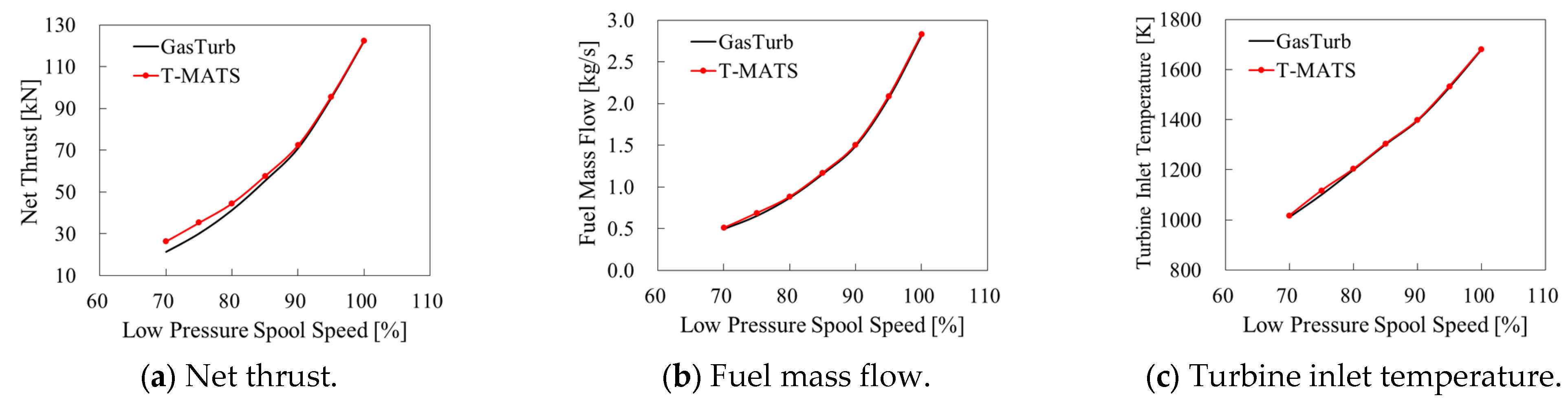
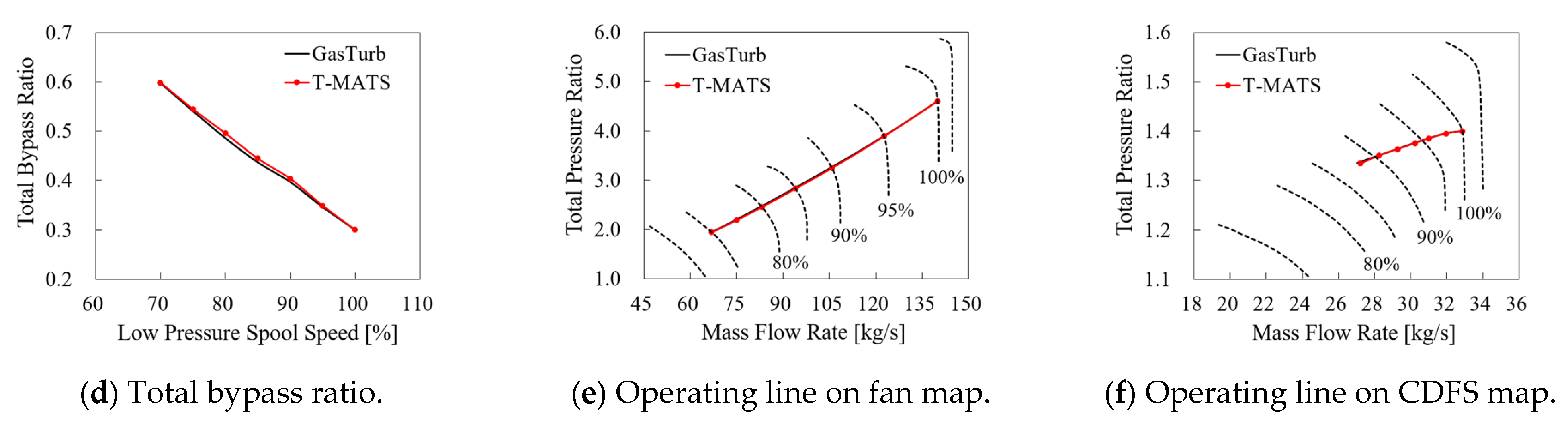
3.3.1. Validation of the ACE Performance Simulation Method

The 0D engine performance model was validated on the double bypass variable cycle engine. As no engine experiment was available to validate the established ACE model in this paper, the accuracy of the model was determined by the health and maturity of the developed modeling methodologies and their results, which showed trends in variation for the most part [37]. Therefore, the developed double-bypass variable-cycle engine was chosen as the object, and the prediction results were compared with those of GasTurb. As shown in Figure 5, the critical performance parameters, including the thrust, fuel mass flow, turbine inlet temperature (T4), total bypass ratio, and the operating lines predicted by T-MATS, show the same trends as those of GasTurb. Except for the thrust deviation at a low rotating speed, which is caused by the use of a different mixed-modeling method, the comparison proves the validity of the modeling methodologies.

The 3D simulation method was validated on a five-stage axial compressor by our team in previous work [38]. The SST model and mixing-plane method were used for the turbulence closure and rotor–stator interface, respectively. TurboGrid was adopted to generate the structured grids, and an H-grid was used for the passage and tip area, while an O-grid was used for the blade area; the same settings were used in this paper for the adaptive fan. Moreover, the experiment was conducted on the five-stage axial compressor. The static and total pressures of the inlet and outlet, the static and total temperatures of the inlet and outlet, and the inlet mass flow rate, rotating speed, and ambient pressure and temperature were measured for analysis. Diaphragm pressure sensors with an error of less than ±0.35 kPa were used for the pressure measurement, a thermocouple with an error of less than ±0.25 K was used for the temperature measurement, a vortex flow meter with a relative error within ±0.5% was used for the mass flow rate measurement, and an electromagnetic transducer with a relative error within ±0.25% was used for the rotating speed measurement. The results are shown in Figure 6. The errors between the experimental and numerical results in the choked mass flow rate, peak pressure ratio, and peak efficiency are about 0.1%, 1.4%, and 1.1%, respectively. Despite some small errors, the trend in the variation of the experimental and numerical results is the same.

Moreover, the 1D mean line model was validated on NASA’s axial turbine by our team in previous work [31]. The empirical coefficients of the 1D mean line model were optimized via the genetic algorithm. The predicted results were compared with the original 1D mean-line model and validated through experiments; they are shown in Figure 7. It can be seen that, in this experiment, the optimized model improved the prediction accuracy by 1.7% with respect to the output power. Then, the optimized 1D model was used to conduct an LPT performance evaluation in this paper.

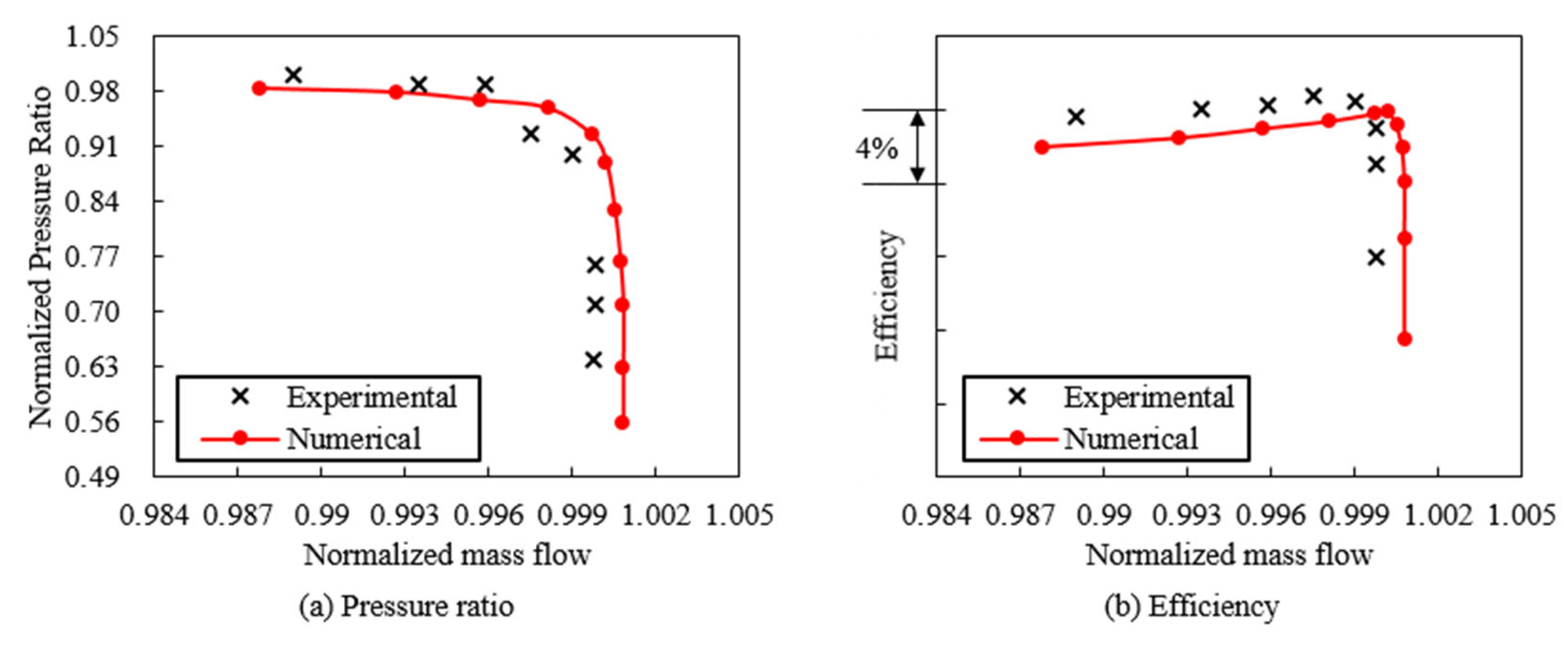
3.3.2. Validation of the Tip Clearance Model

In this section, the 3D FSTM was adopted to validate the prediction accuracy of the tip clearance prediction model for the adaptive fan and turbine. The fan rotors, shroud structure, and shroud coating are made of an Al7075 alloy, austenitic chromium–nickel stainless steel, and zirconium oxide, respectively. In the design case, the rotating speed is 49,000 revolutions per minute (RPM), and the assembled clearance is 0.3 mm. Moreover, the computational domain and the mesh of the front fans for a conjugate heat transfer (CHT) analysis are shown in Figure 8, and those of the rear fan are similar.

After the CHT analysis, the component deformations were predicted via a thermal–structural analysis at the rotating speed of the design case, and the results of the front and rear fans are shown in Figure 9. Furthermore, a comparison of component deformations and tip clearance between the multi-dimensional tip clearance model (MDM) and the FSTM of the front and rear fans are shown in

Table 4. Deformation and tip clearance prediction comparisons for the front fan.

	Shroud Deformation	Blade Deformation	Disk Deformation	Tip Clearance
MDM	0.10 mm	0.18 mm	0.12 mm	0.10 mm
FSTM	0.14 mm	0.22 mm	0.12 mm	0.10 mm
Difference	−0.04 mm	−0.04 mm	0 mm	0 mm

and

Table 5. Deformation and tip clearance prediction comparisons for the rear fan.

	Shroud Deformation	Blade Deformation	Disk Deformation	Tip Clearance
MDM	0.16 mm	0.15 mm	0.22 mm	0.09 mm
FSTM	0.18 mm	0.14 mm	0.21 mm	0.13 mm
Difference	−0.02 mm	+0.01 mm	+0.01 mm	−0.04 mm

. It can be concluded from the tables that the difference between the MDM and FSTM is small (not exceeding 0.04 mm), and the MDM can be a useful tool for tip clearance prediction.

The results for turbines are similar to the results for fans. The main difference lies in considering the heat transfer of the disk cavity and the cooling of the blade film. The author adopted the FSTM to validate the variation in the transient tip clearance in another case with an assembled clearance of 0.2 mm, considering the heat transfer of the disk cavity [17]. Furthermore, the computational domain of the turbine for a CHT analysis is shown in Figure 10. Moreover, the comparison results of the predicted steady-state deformations and tip clearance among the 1 DM (one-dimensional tip clearance model), MDM, and FSTM, and the computational cost of the entire variation process are shown in

Table 6. Comparison of deformation and tip clearance predictions for the turbine.

	Shroud Deformation	Blade Deformation	Disk Deformation	Tip Clearance	Time	Cores
1 DM	1.18 mm	0.45 mm	0.17 mm	0.76 mm	20 min	4
MDM	1.00 mm	0.35 mm	0.36 mm	0.49 mm	120 min	4
FSTM	0.97 mm	0.30 mm	0.30 mm	0.57 mm	18,000 min	40

. It can be concluded from the table that the difference between the MDM and FSTM is 0.11 mm smaller than the difference between the 1 DM and FSTM, and the computational cost of the MDM is only 1/1500 of the FSTM.

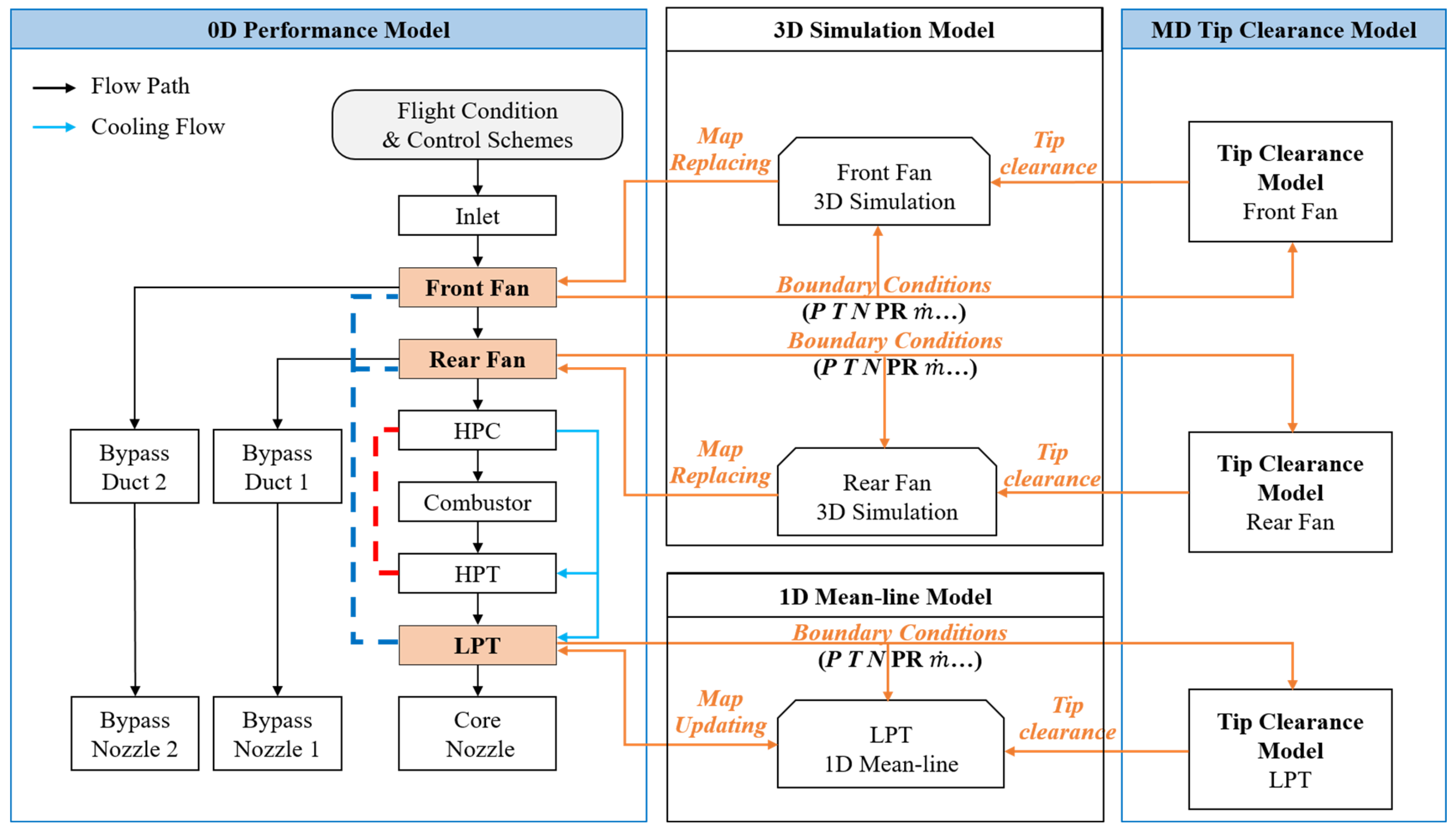
3.4. The Integration of the Models

An ACE performance simulation system that considers the impact of variations in tip clearance was established and is shown in Figure 11. The architecture of the whole system shows the following:

• The ACE’s performance in double-bypass mode is calculated through the 0D performance model. Furthermore, it provides boundary conditions for the 3D simulation model of the front and rear fans, the 1D mean line model of the LPT, and the MD tip clearance model of the fans and the LPT.
• The MD tip clearance model provides the predicted tip clearances for the front and rear fans and the LPT under different rotating speeds. Moreover, the boundary conditions for the tip clearance model originate from the 0D performance model, including the temperature and mass flow rate of the airflow through the components and the rotating speed.
• The 3D simulation model calculates the impact of clearance variations on the characteristic maps of the front and rear fans, using the tip clearances from the clearance model and the boundary conditions from the 0D performance model. The new maps are then used to replace the front and rear fan maps in the 0D performance model.
• The 1D mean line model is used to calculate the impact of variations in tip clearance on the performance of the LPT, using the tip clearances from the clearance model and the boundary conditions from the 0D engine model. The map is then updated and processed for the LPT, meaning that several iterations between the 0D performance model and the 1D mean line model are processed to calculate the LPT’s performance.
• Finally, the engine performance considering the effect of variations in the tip clearance can be obtained.

4. Results Analysis

In this section, the results of the prediction of the tip clearance model at each rotating speed are calculated, and the characteristic maps of the adaptive fan and the LPT, which consider the influence of variations in the tip clearance, are analyzed. Then, changes in the performance of the ACE between the engine with an assembled clearance of 0.3 mm and the engine with the predicted tip clearance were compared. Moreover, the performance results calculated under the assembled tip clearance are designated as the design values, while the performance results calculated under the predicted tip clearance are designated as the predicted values.

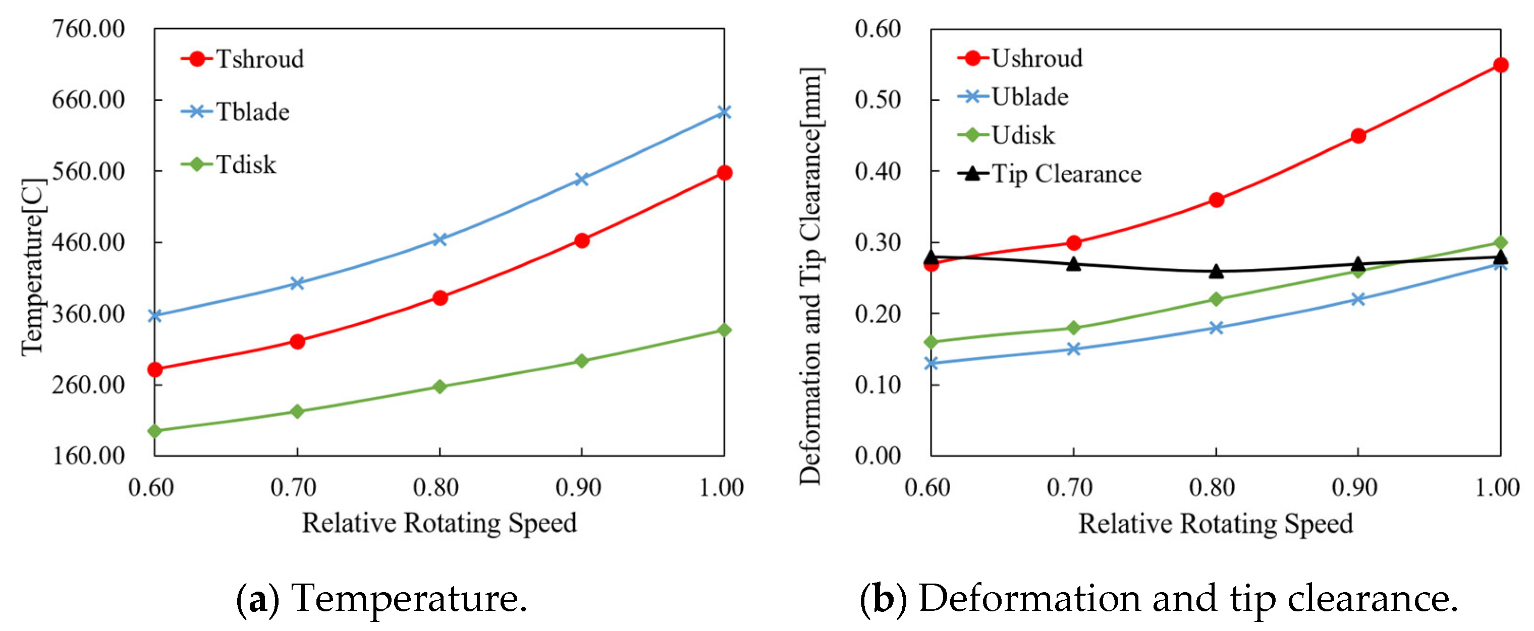
4.1. Tip Clearance Model Prediction Results

The results of the variations in tip clearance under different rotating speeds were calculated based on the boundary conditions provided by the 0D engine performance simulation model. Moreover, the wall of the fan disk was considered adiabatic, and heat conduction from the shaft to the disk was considered. Furthermore, the turbine disk and blade were cooled by bleeding air from the middle stage of the high-pressure compressor, and the outer wall of the turbine shroud was cooled by the first bypass nozzle.

The components’ temperature, the components’ deformation, and the tip clearance prediction results for the front fan are shown in Figure 12, as follows:

In Figure 12, Tshroud, Tblade, and Tdisk denote the shroud, blade, and disk temperature. Moreover, Ushroud, Ublade, and Udisk denote the shroud, blade, and disk deformation. As can be seen from this figure, the component temperature and deformation increase as the rotating speed increases. In addition, the overall temperature of the front fan is low, so the deformation caused by centrifugal force is relatively large. Therefore, the sum of the deformation of the blade and disk is larger than that of the shroud, resulting in a tighter clearance as the rotating speed increases.

The components’ temperature, the components’ deformation, and the tip clearance prediction results for the rear fan are shown in Figure 13, as follows:

As shown in Figure 13, similar to the results for the front fan, the sum of the deformation of the blade and disk is larger than that of the shroud, resulting in a tighter clearance as the rotating speed increases.

The components’ temperature, the components’ deformation, and the tip clearance prediction results for the LPT are shown in Figure 14, as follows:

As shown in Figure 14, differing from the deformation of the adaptive fan, the cooling effect of the outer wall of the turbine shroud effectively controls the growth of the shroud, and the sum of the deformation of the blade and disk is close to that of the shroud. Therefore, the turbine’s tip clearance mostly remains the same at different rotating speeds.

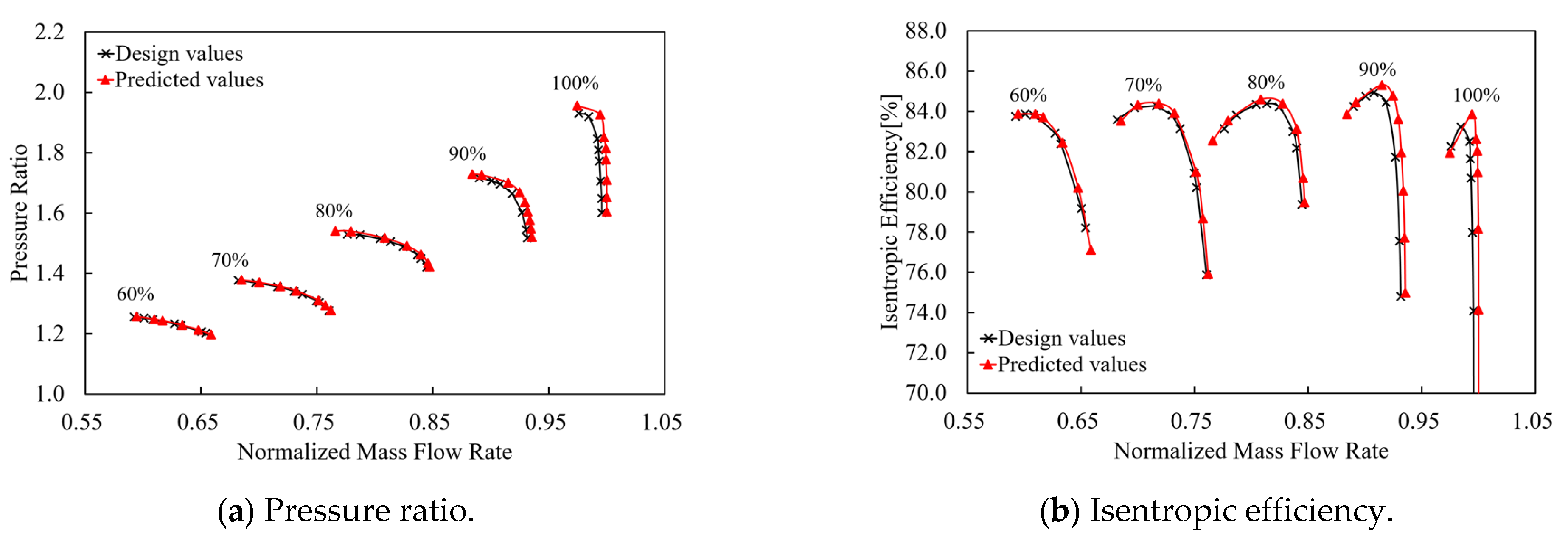
4.2. Characteristic Maps of the Adaptive Fan

The 3D numerical simulation was adopted for the characteristic maps of the front and rear fans, respectively.

The characteristic maps of the front fan at different rotating speeds are shown in Figure 15. The mass flow rate is normalized by the choked mass flow rate of the design case. As the figure shows, the tip clearance decreases at a high rotating speed, reducing the tip leakage vortex. Hence, the predicted choked mass flow rate of the fan is larger than the design value. Moreover, the pressure ratio and the isentropic efficiency increase. For example, at 100% of the rotating speed, compared with the design value of the front fan, the predicted choked mass flow rate, peak pressure ratio, and peak efficiency increase by 0.4%, 1.3%, and 0.6%, respectively. However, at lower rotating speeds, the change in the characteristic line is less due to the small variation in the tip clearance.

The characteristic maps of the rear fan at different rotating speeds were calculated. Meanwhile, to introduce the variable-geometry characteristics of the ACE, characteristic maps of different inlet flow angles of the rear fan were calculated from −20° to 0°. The mass flow rate was normalized by the choked mass flow rate of the design case at an inlet flow angle of 0°. The rear fan at an inlet flow angle of 0° is shown in Figure 16. As the figure shows, the tip clearance decreases at a high rotating speed, reducing tip leakage vortex, similar to the front fan case. Moreover, at 100% of the rotating speed, compared with the design value of the rear fan, the predicted choked mass flow rate, peak pressure ratio, and peak efficiency increase by 0.1%, 0.3%, and 1.0%, respectively. Furthermore, the rear fan at an inlet flow angle of −20° is shown in Figure 17. As the figure shows, at 100% of the rotating speed, compared with the value of the rear fan in the design case, the predicted choked mass flow rate, peak pressure ratio, and peak efficiency increase by 0.1%, 0.4%, and 1.0%, respectively.

Still, at lower rotating speeds, especially at 70% of the rotating speed or less, the change in the characteristic line is smaller due to the small variation in the tip clearance. The characteristic maps of other inlet flow angles of the rear fan are similar.

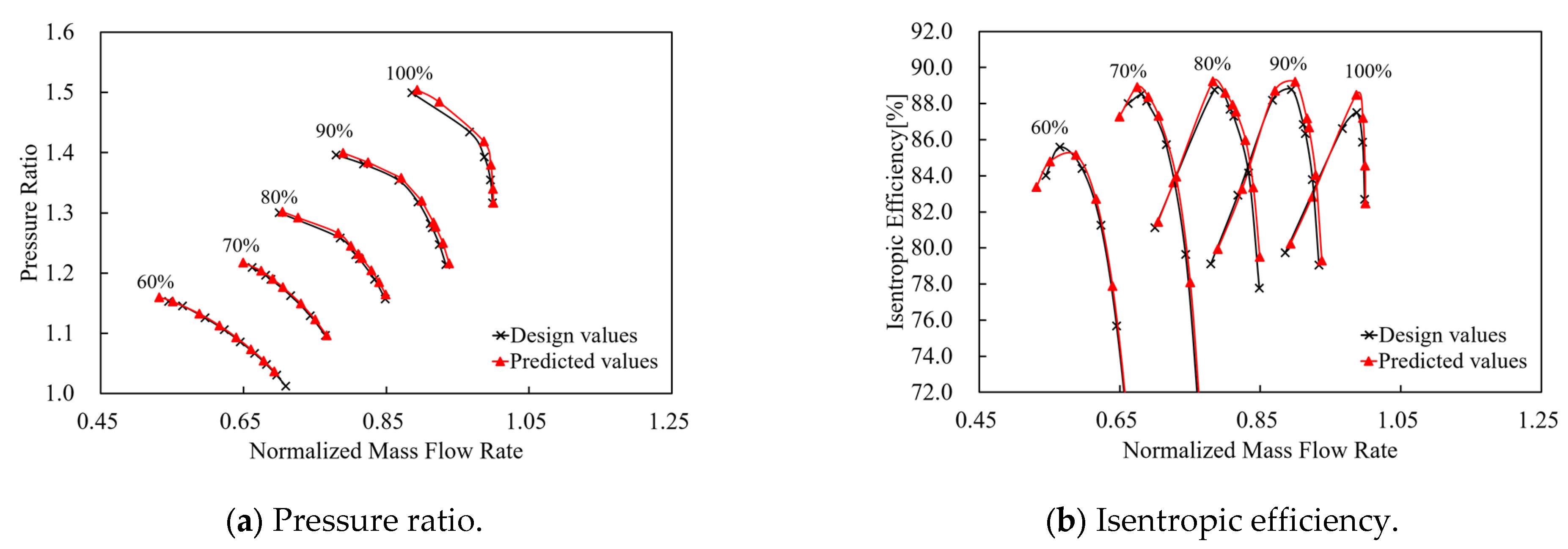
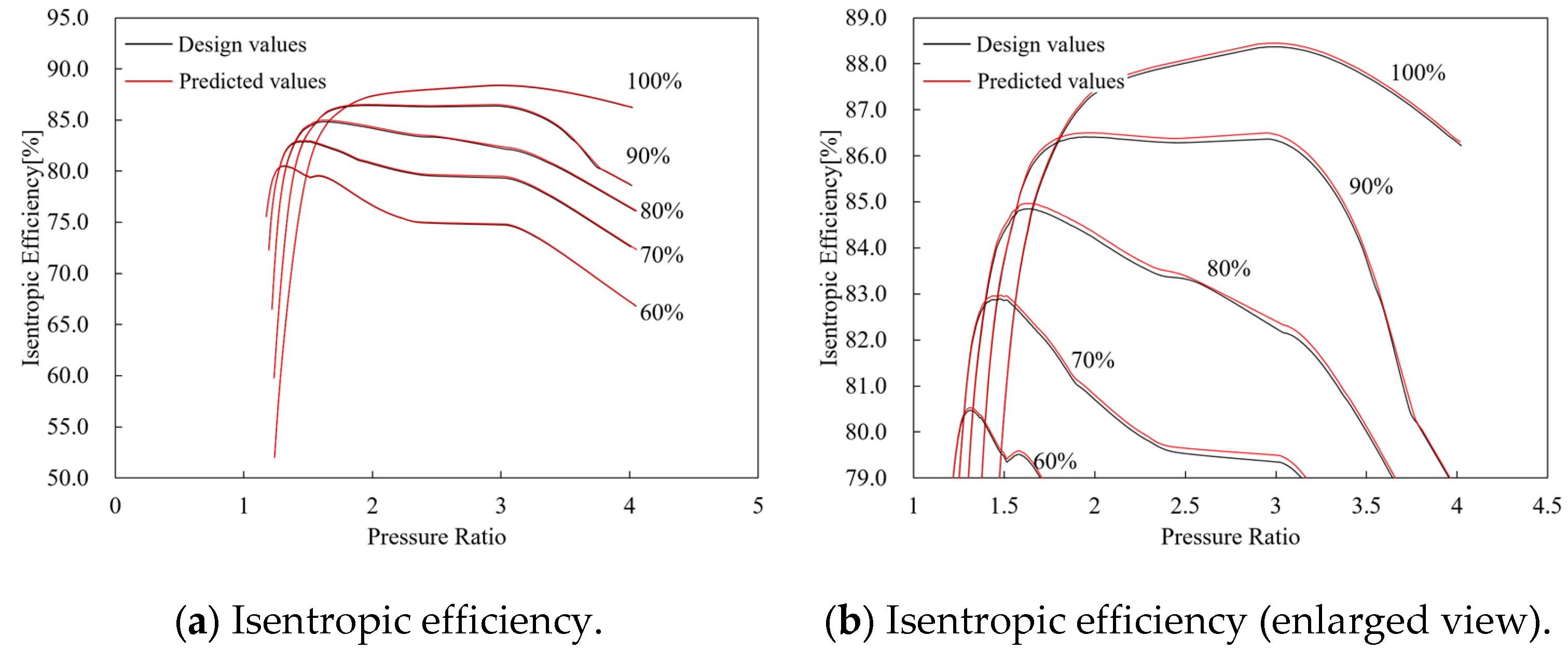
4.3. Characteristic Maps of the LPT

The iteratively coupled method was used to determine variations in the performance of the LPT, meaning that iterations between the 0D performance model and the 1D mean line model were processed to calculate the performance of the LPT. Meanwhile, to show the impact of variations in tip clearance on the LPT, characteristic maps of the LPT at different rotating speeds and an enlarged view of the LPT are shown in Figure 18. As the figure shows, the predicted LPT efficiency is higher than the value for the design case. The difference in the maximum efficiency is approximately 0.2% at high rotating speeds. However, at lower rotating speeds, especially under 70% of the rotating speed, the difference decreases to 0.05%. The difference in the efficiency of the LPT is small because the tip clearance difference is less than 0.04 mm (0.15% of the blade height). If the tip clearance variation increases as the difference of each component’s deformation increases, for example, when the cooling air temperature of the shroud changes, the efficiency difference could be large.

4.4. Engine Performance Evaluation

After introducing the influence of the tip clearance, the integrated model was used to compare the performance of the ACE between the assembled tip clearance and the predicted tip clearance. Similarly, the performance calculated for the assembled tip clearance is designated as the design value, while the performance calculated for the predicted tip clearance is designated as the predicted value.

Firstly, the design and predicted operating characteristics of the ACE in double-bypass mode were compared. Figure 19 shows the characteristic maps of the front fan with an inlet flow angle of 0°, the rear fan with an inlet flow angle of 0°, and the movement of the operating line of the engine. The inlet flow angle of the rear fan needs to be adjusted according to the outlet condition of the front fan, as shown in

Table 7. Control schemes of the variable geometry.

Low-Pressure Spool Relative Speed	100%	90%	80%	70%	60%
Front fan inlet flow angle (deg)	0	0	0	0	0
Rear fan inlet flow angle (deg)	0	−5	−10	−15	−20
Throat area of the 1st bypass nozzle (%)	0	5	10	15	20
Throat area of the 2nd bypass nozzle (%)	0	15	30	45	60

. Furthermore, only the rear fan map with an inlet flow angle of 0° is displayed here. It can be seen from the figure that the shape of the operating line hardly changes between the two cases. However, due to the change in the characteristic map, the position of the operating point moves toward the direction of the larger mass flow rate and higher-pressure ratio. Taking 100% speed as an example, the operating point of the front fan changes from the normalized mass flow rate of 0.993 to 0.999, and the pressure ratio changes from 1.802 to 1.804. Furthermore, the operating point of the rear fan changes from the normalized mass flow rate of 0.973 to 0.979, and the pressure ratio changes from 1.422 to 1.431. The pressure ratio change is small due to the selection of the design case’s operating point at a lower pressure ratio. However, the change in the pressure ratio of the front fan could exceed 1% if the design case’s operating point is set at the peak pressure point. The characteristic maps of the rear fan at other inlet flow angles are similar.

The performance of the engine with two tip clearances was further analyzed, and the thrust, specific fuel consumption (SFC), and T4 under different rotating speeds were compared, as shown in Figure 20. Finally, the difference is presented in

Table 8. Difference in engine performance at different rotating speeds.

Low-Pressure Spool Relative Speed	100%	90%	80%	70%	60%
Net thrust difference	1.0%	1.3%	0.8%	0.6%	0.5%
SFC difference	−0.3%	−0.2%	−0.2%	−0.3%	−0.2%
T4 difference	−0.2 K	3.0 K	1.4 K	0.4 K	0.4 K

. It can be seen from the table that, considering the variation in the tip clearance, the predicted thrust, SFC, and T4 all change. For example, at 100% rotating speed, the thrust difference can reach 1%, the SFC difference is −0.3%, and the T4 difference is −0.2 K. Therefore, the changes in the tip clearance during operation cannot be ignored. They should be considered when predicting the performance of an ACE.

5. Conclusions

This paper aimed to solve the problem of considering the impact of tip clearance on the ACE and further improving its thrust and fuel consumption prediction accuracy. A new integrated model for predicting the performance of an ACE was established, and the conclusions can be drawn as follows:

• This paper developed a new integrated model for predicting the performance of an ACE, including a 0D engine performance simulation model, a 3D adaptive fan numerical simulation model, a 1D LPT mean line model, and an MD tip clearance prediction model. Specifically, the 0D model provides the boundary conditions for the 1D LPT, 3D adaptive fan, and MD tip clearance models. Then, the MD tip clearance model provides the predicted clearances for the 3D adaptive fan and 1D LPT models, so the impact of the variation in tip clearance on the components can be considered. Finally, after replacing the map of the adaptive fan and updating the map of the LPT, the ACE performance can be obtained while considering the effect of the variant clearance.
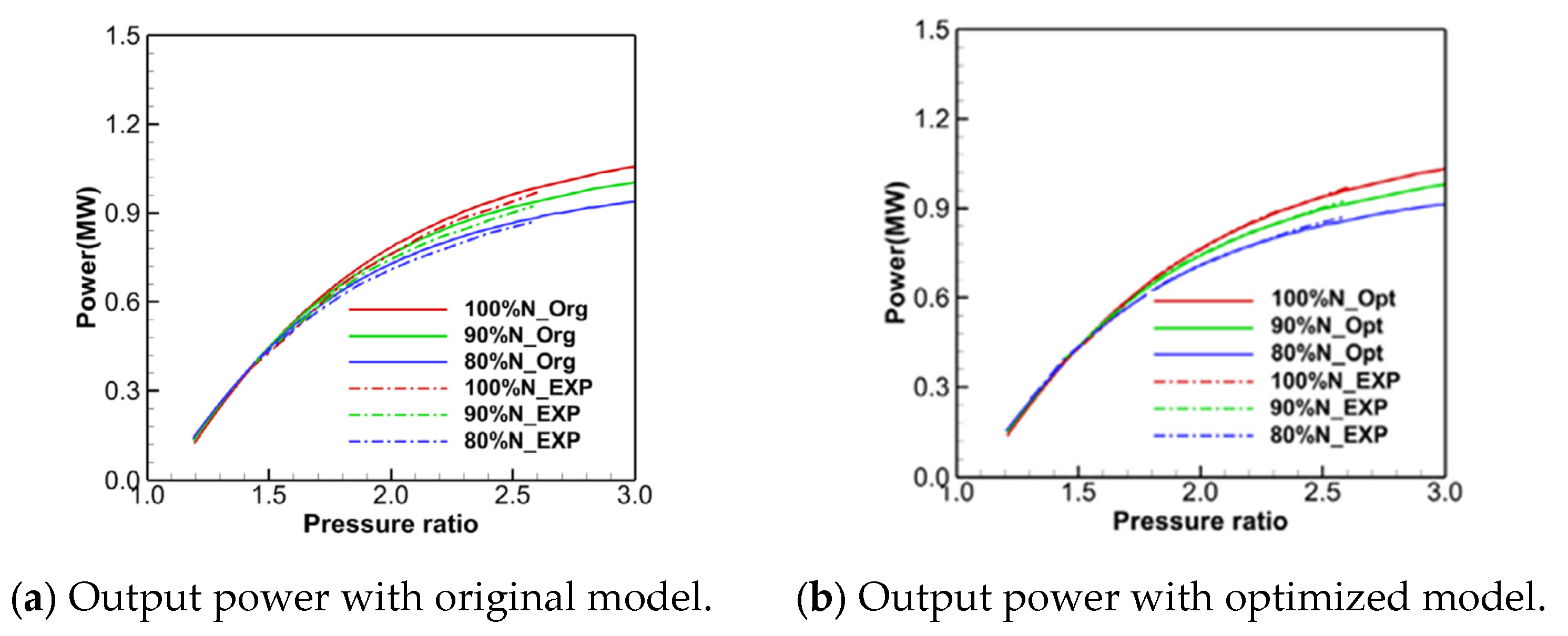
• The traditional 0D engine performance model mainly adopts empirical relations and variable multi-angle characteristic maps for predicting the maps of the components, which usually cannot meet the design and analysis requirements of engineers and researchers for the ACE. The new integrated model combines high-fidelity models of the adaptive fan and LPT, and the accuracy of the adaptive fan and LPT model was validated via experiments. Moreover, the MD tip clearance model, validated via the 3D FSTM, further improves the accuracy of the prediction of the ACE’s performance, as it considers the variation in the tip clearance under different operating conditions.
• The integrated model calculated the performance of the ACE considering variations in the tip clearance under different operating conditions, and the results were compared with the performance of an ACE with the assembled clearance values. When compared with the performance of the ACE without considering the clearance variations, the thrust under the design conditions increased by 1%, and the SFC decreased by 0.3%. Moreover, this indicates that the impact of tip clearance on the performance of an ACE cannot be ignored.

References

- Westmoreland, J.S.; Howlett, R.A.; Lohmann, R.P. Progress on Variable Cycle Engines. In Proceedings of the 15th Joint Propulsion Conference, Las Vegas, NV, USA, 18–20 June 1979. [Google Scholar]
- Claus, R.W.; Evans, A.L.; Lylte, J.K.; Nichols, L.D. Numerical Propulsion System Simulation. Comput. Syst. Eng. 1991, 2, 357–364. [Google Scholar] [CrossRef]
- Alexiou, A.; Baalbergen, E.H.; Kogenhop, O.; Mathioudakis, K.; Arendsen, P. Advanced Capabilities for Gas Turbine Engine Performance Simulations. In Proceedings of the ASME Turbo Expo 2007: Power for Land, Sea, and Air, Montreal, QC, Canada, 14–17 May 2007. [Google Scholar]
- Kim, S.; Kim, D.; Son, C.; Kim, K.; Kim, M.; Min, S. A Full Engine Cycle Analysis of a Turbofan Engine for Optimum Scheduling of Variable Guide Vanes. Aerosp. Sci. Technol. 2015, 47, 21–30. [Google Scholar] [CrossRef]
- Follen, G.; AuBuchon, M. Numerical Zooming between a NPSS Engine System Simulation and a One-Dimensional High Compressor Analysis Code; NASA/TM-2000-209913; NASA: Washington, DC, USA, 2000.
- Kolias, I.; Alexiou, A.; Aretakis, N.; Mathioudakis, K. Axial Compressor Mean-Line Analysis: Choking Modelling and Fully-Coupled Integration in Engine Performance Simulations. Int. J. Turbomach. Propuls. Power 2021, 6, 4. [Google Scholar] [CrossRef]
- Pilet, J.; Lecordix, J.L.; Garcia-Rosa, N.; Barènes, R.; Lavergne, G. Towards a Fully Coupled Component Zooming Approach in Engine Performance Simulation. In Proceedings of the ASME Turbo Expo 2011: Power for Land, Sea, and Air, Vancouver, BC, Canada, 6–10 June 2011. [Google Scholar]
- Klein, C.; Wolters, F.; Reitenbach, S.; Schönweitz, D. Integration of 3D-CFD Component Simulation into Overall Engine Performance Analysis for Engine Condition Monitoring Purposes. In Proceedings of the ASME Turbo Expo 2018: Power for Land, Sea, and Air, Oslo, Norway, 11–15 June 2018. [Google Scholar]
- Zhewen, X.; Ming, L.; Hailong, T.; Chen, M. A Multi-Fidelity Simulation Method Research on Front Variable Area Bypass Injector of an Adaptive Cycle Engine. Chin. J. Aeronaut. 2022, 35, 202–219. [Google Scholar]
- Fu, S.; Li, Z.; Zhanxue, W.; Lin, Z.; Shi, J. Integration of High-Fidelity Model of Forward Variable Area Bypass Injector into Zero-Dimensional Variable Cycle Engine Model. Chin. J. Aeronaut. 2021, 34, 1–15. [Google Scholar]
- Ameri, A.A.; Steinthorsson, E.; Rigby, D.L. Effects of Tip Clearance and Casing Recess on Heat Transfer and Stage Efficiency in Axial Turbines. J. Turbomach. 1999, 121, 683–693. [Google Scholar] [CrossRef]
- Bringhenti, C.; Barbosa, J.R. Effects of Turbine Tip Clearance on Gas Turbine Performance. In Proceedings of the ASME Turbo Expo 2008: Power for Land, Sea, and Air, Berlin, Germany, 9–13 June 2008. [Google Scholar]
- Lattime, S.B.; Steinetz, B.M. High Pressure Turbine Engine Clearance Control Systems: Current Practices and Future Directions. J. Propuls. Power 2004, 20, 302–311. [Google Scholar] [CrossRef]
- Ebert, E.; Reile, E. Bridging The Gap between Structural and Thermal Analysis in Aircraft Engine Design. In Proceedings of the 8th AIAA/USA/NASA/ISSMO Symposium on Multidisciplinary Analysis and Optimization, Long Beach, CA, USA, 6–8 September 2000. [Google Scholar]
- Yu, Y.; Liu, Q.; Shen, B.; Gao, X. Radical Clearance Analysis on the High Pressure Compressor. In Proceedings of the 18th AIAA/3AF International Space Planes and Hypersonic Systems and Technologies Conference, Tours, France, 24–28 September 2012. [Google Scholar]
- Kumar, R.; Kumar, V.S.; Butt, M.M.; Sheikh, N.A.; Khan, S.A.; Afzal, A. Thermo-Mechanical Analysis and Estimation of Turbine Blade Tip Clearance of a Small Gas Turbine Engine under Transient Operating Conditions. Appl. Therm. Eng. 2020, 179, 115700. [Google Scholar] [CrossRef]
- Wei, J.; Yang, H.; Zheng, P.; Wang, B.; Zheng, X. Transient Tip Clearance Prediction Model Considering Transient Radial Temperature Distribution of Discs in a Gas Turbine Engine. In Proceedings of the ASME Turbo Expo 2023, Boston, MA, USA, 26–30 June 2023. in press. [Google Scholar]
- Pilidis, P.; Maccallum, N.R.L. A Study of the Prediction of Tip and Seal Clearances and Their Effects in Gas Turbine Transients. In Proceedings of the ASME 1984 International Gas Turbine Conference and Exhibit, Amsterdam, The Netherlands, 4–7 June 1984. [Google Scholar]
- Kypuros, J.A.; Melcher, K.J. A Reduced Model for Prediction of Thermal and Rotational Effects on Turbine Tip Clearance; NASA/TM–2003–212226; NASA: Washington, DC, USA, 2003.
- Agarwal, H.; Akkaram, S.; Shetye, S.; McCallum, A. Reduced Order Clearance Models for Gas Turbine Applications. In Proceedings of the 49th AIAA/ASME/ASCE/AHS/ASC Structures, Structural Dynamics, and Materials Conference, Schaumburg, IL, USA, 7–10 April 2008. [Google Scholar]
- Chapman, J.W.; Guo, T.H.; Kratz, J.L.; Litt, J.S. Integrated Turbine Tip Clearance and Gas Turbine Engine Simulation. In Proceedings of the 52nd AIAA/SAE/ASEE Joint Propulsion Conference, Salt Lake City, UT, USA, 25–27 July 2016. [Google Scholar]
- Peng, K.; Fan, D.; Yang, F.; Fu, Q.; Li, Y. Active Generalized Predictive Control of Turbine Tip Clearance for Aero-Engines. Chin. J. Aeronaut. 2013, 26, 1147–1155. [Google Scholar] [CrossRef]
- Dong, Y.; Xinqian, Z.; Qiushi, L. An 11-Stage Axial Compressor Performance Simulation Considering the Change of Tip Clearance in Different Operating Conditions. Proc. IMechE Part A J. Power Energy 2014, 228, 614–625. [Google Scholar] [CrossRef]
- Luberti, D.; Tang, H.; Scobie, J.A.; Pountney, O.J.; Owen, J.M.; Lock, G.D. Influence of Temperature Distribution on Radial Growth of Compressor Disks. J. Eng. Gas. Turbines Power 2020, 142, 071004. [Google Scholar] [CrossRef]
- Youlong, F.; Yongbao, L.; Xing, H. Study of the Radial Elongations of the Turbine Rotor with the Centrifugal Effect. Ship Electron. Eng. 2011, 31, 177–180. [Google Scholar]
- Vullo, V.; Vivio, F. Rotors: Stress Analysis and Design; Springer: Berlin, Germany, 2013. [Google Scholar]
- Johnson, J.E. Variable Cycle Engine Developments at General Electric-1955–1995. In Murthy S N B, Curran E T. Developments in High-Speed Vehicle Propulsion Systems; AIAA Inc.: Reston, VA, USA, 1996; pp. 105–158. [Google Scholar]
- Chapman, J.W.; Lavelle, T.M.; May, R.D.; Litt, J.S.; Guo, T.-H. Toolbox for The Modeling and Analysis of Thermodynamic Systems (T-MATS) User’s Guide; NASA/TM-2014-216638; NASA: Washington, DC, USA, 2014.
- Edmunds, D.B. Multivariable Control for a Variable Area Turbine Engine. Master’s Dissertation, Ohio State University, Columbus, OH, USA, 1977. [Google Scholar]
- Grönstedt, T. Development of Methods for Analysis and Optimization of Complex Jet Engine Systems. Ph.D. Dissertation, Chalmers University of Technology, Gothenburg, Sweden, 2000. [Google Scholar]
- Wang, B.; Song, Z.; Zou, W.; Yang, H.; Wen, M.; Zhou, K.; Feng, X.; Zheng, X. Rapid Performance Prediction Model of Axial Turbine with Coupling One-Dimensional Inverse Design and Direct Analysis. Aerosp. Sci. Technol. 2022, 130, 107828. [Google Scholar] [CrossRef]
- Kacker, S.C.; Okapuu, U. A Mean Line Prediction Method for Axial Flow Turbine Efficiency. J. Eng. Power 1982, 104, 111–119. [Google Scholar] [CrossRef]
- Zhu, J.; Sjolander, S.A. Improved Profile Loss and Deviation Correlations for Axial-Turbine Blade Rows. In Proceedings of the ASME Turbo Expo 2005: Power for Land, Sea, and Air, Reno-Tahoe, NV, USA, 6–9 June 2005. [Google Scholar]
- Agromayor, R.; Nord, L.O. Preliminary Design and Optimization of Axial Turbines Accounting for Diffuser Performance. Int. J. Turbomach. Propuls. Power 2019, 4, 32. [Google Scholar] [CrossRef]
- Incropera, F.P.; DeWitt, D.P. Fundamentals of Heat and Mass Transfer; John Wiley & Sons: New York, NY, USA, 1996. [Google Scholar]
- Tachibana, F.; Fukui, S. Convective Heat Transfer of the Rotational and Axial Flow between Two Concentric Cylinders. Bull. JSME 1958, 7, 385–391. [Google Scholar] [CrossRef]
- Kopasakis, G.; Cheng, L.; Connolly, J.W. Stage-by-Stage and Parallel Flow Path Compressor Modeling for a Variable Cycle Engine. In Proceedings of the 51st AIAA/SAE/ASEE Joint Propulsion Conference, Orlando, FL, USA, 27–29 July 2015. [Google Scholar]
- Zheng, X.; Yang, H. Influence of Tip Clearance on the Performance and Matching of Multistage Axial Compressors. In Proceedings of the ASME Turbo Expo 2016: Turbomachinery Technical Conference and Exposition, Seoul, Republic of Korea, 13–17 June 2016. [Google Scholar]