Exploring Bayesian Optimization for Photocatalytic Reduction of CO₂

Abstract

The optimization of photocatalysis is complex, as heterogenous catalysis makes its kinetic modeling or design of experiment (DOE) significantly more difficult than homogeneous reactions. On the other hand, Bayesian optimization (BO) has been found to be efficient in the optimization of many complex chemical problems but has rarely been studied in photocatalysis. In this paper, we developed a BO platform and applied it to the optimization of three photocatalytic CO₂ reduction systems that have been kinetically modeled in previous studies. Three decision variables, namely, partial pressure of CO₂, partial pressure of H₂O, and reaction time, were used to optimize the reaction rate. We first compared BO with the traditional DOE methods in the Khalilzadeh and Tan systems and found that the optimized reaction rates predicted by BO were 0.7% and 11.0% higher, respectively, than the best results of optimization by DOE, and were significantly better than the original experimental data, which were 1.9% and 13.6% higher, respectively. In both systems, we also explored the best combination of the surrogate model and acquisition function for BO, and the results showed that the combination of Gaussian processes (GP) and upper confidence bound (UCB) had the most stable search performance. Furthermore, the Thompson system with time dependence was optimized with BO according to the selectivity of CH₄. The results showed that the optimized reaction time of BO agreed with the actual experimental data with an error of less than 5%. These results suggest that BO is a more promising alternative to kinetic modeling or traditional DOE in the efficient optimization of photocatalytic reduction.

1. Introduction

The conversion of CO₂ into high-value-added sustainable chemicals and fuels (e.g., CH₄) using photocatalytic reduction [1] has become one of the effective solutions for chemists worldwide to address the challenges of global warming and the energy crisis. As different photocatalytic systems have different catalysts, light sources, and photoreactors, the scale and geometry-independent Langmuir–Hinshelwood (hereafter L-H) kinetic model has been widely used to correlate experimental data and as a benchmark to describe the performance of photocatalytic CO₂ reduction. In this context, a heterogeneous photocatalytic kinetic model was developed by Tan et al. [2]. For catalysts with different energy sites, Khalilzadeh et al. [3] developed a kinetic model based on the sips [4] isotherm. Thompson et al. [5] responded to the challenge of catalyst deactivation by developing a new CO₂ photoreduction kinetic for a selectivity model for different products (CH₄, CO, H₂). Currently, kinetic models of conventional photocatalytic systems have limited generality, and small changes in catalyst and experimental variables [6,7] can render the model ineffective. Furthermore, reconstructing a model [8] is often time-consuming and costly. In the case of heterogeneous photocatalytic [9] systems involving adsorption processes, kinetic models require more parameters, which makes model tuning more difficult and increases the computational effort. In addition, more decision variables [10], such as light level, temperature, and pressure, further add to the complexity and difficulty of optimizing photocatalytic systems. Therefore, there is an urgent need for more economical and effective optimization methods for photocatalytic reduction research.

Design of experiment (DOE) has been widely used in process flow and quality control due to its advantages of low cost, high quality, and short test period. Paul et al. [11] used a resolution IV DOE method to optimize SNAr reaction; Randall et al. [12] successfully applied the fractional factorial (FF) DOE method in the study of biological in vitro culture. Lee et al. [13] explained the application of the central composite design (CCD) DOE method in environmental chemistry. Anika et al. [14] successfully implemented the full factorial design (FFD) DOE method in furniture and other manufacturing industries. DOE seeks key factors and control-related factors through quantitative analysis of process parameters. However, DOE is not suitable for high-dimensional variable space [15], especially in the mixed domain with category variables. As the number of experiments required by the DOE method increases exponentially with the number of factors, factor screening [16] must be carried out. In addition, DOE tests continuous variables with predefined values, so the optimal value between these values will likely be missed [17]. Moreover, in DOE, the data obtained from the previous batches of experiments do not influence the selection of variable combinations for the next batch. Therefore, these limitations of DOE may prevent it from efficiently optimizing complex reaction systems like photocatalytic reduction.

Bayesian optimization (BO) is a statistics-based global optimization algorithm that has been used to solve optimization problems with high evaluation costs, such as multimodal [18], nonconvex objectives [19], and observed noise [20], due to its powerful generalization performance [21]. It mainly consists of the surrogate model and the acquisition function. BO constantly updates the fitting of the surrogate model with previously obtained data and determines the next most “potential” evaluation point [22] based on the optimization of acquisition functions. In recent years, chemists have used the BO algorithm for applications in chemical reactions and processes [23,24]. Doyle et al. [25] applied BO to optimize Mitsunobu and defluorination reactions; Aspuru-Guzik et al. [26] used a closed-loop system developed with BO algorithms to optimize stereoselective Suzuki–Miyaura coupling reactions. In material sciences-related research fields, Deshwal et al. [27] successfully found covalent organic frameworks (COFs) with the highest simulated methane transport capacity through BO in a database consisting of about 70,000 hypothetical COFs; Neaton et al. [28] conducted a proof-of-concept study using BO on the methane absorption capacity of an existing hypothetical metal–organic frameworks (MOFs) dataset; Xie et al. [29] built an intelligent platform combining BO algorithms with synthetic robots to accelerate the synthesis of MOFs. However, research on BO for photocatalytic reduction has rarely been conducted. Traditional experiments for photocatalytic CO₂ reduction are often costly, and repeat experiments usually use the univariate control method, which results in low efficiency. However, the BO method [30] is a low-cost and relatively efficient alternative with the ability to optimize multiple variables at the same time while seeking the optimal value. As a result, the use of BO methods for photocatalytic reduction has the potential to significantly advance the field.

In this study, we aimed to demonstrate the plausibility of utilizing BO photocatalytic reduction of CO₂ to convert it into CH₄. Initially, BO was performed on two photocatalytic reduction systems, with the partial pressure of reactants serving as the decision variable. The outcomes were then compared with those of the conventional DOE method. We also explored the impact of various alternate models and acquisition functions on the photocatalytic BO model. In addition, we optimized a photocatalytic reduction system with three variables, including catalyst deactivation time, to demonstrate the capability of BO in optimizing time-sensitive photocatalysis.

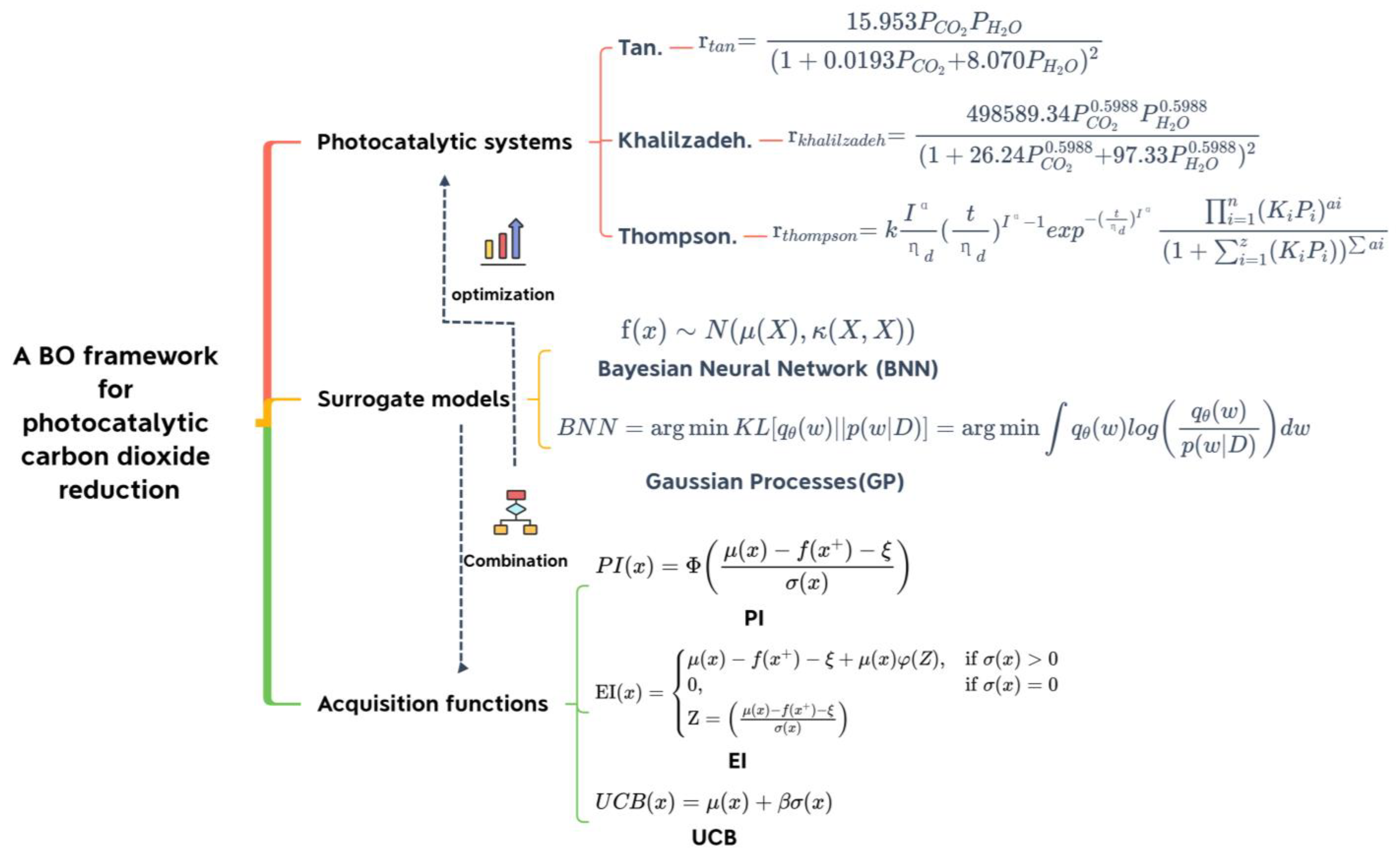
2. Methods and Models

2.1. Optimization Methods

2.1.1. Bayesian Optimization

BO uses the famous Bayesian theorem (see Equation (1)) in the optimization process [22] where $H$ represents the unknown objective function $f\left(x\right)$ (or represents the parameters in the parametric model); $D=\left\{\left(x_1,y_1\right),\left(x_2,y_2\right),\dots ,\left(x_n,y_n\right)\right\}$ represents the observed dataset; $P\left(D\right|H)$ represents the likelihood probability distribution of f(x), which is also called “noise” due to unavoidable errors in the observation; P(H) represents the prior probability distribution, that is, the assumption of $f\left(x\right)$; $P\left(D\right)$ is expressed as the marginal likelihood distribution or “evidence” of the unknown objective function $f\left(x\right)$, for which it is usually challenging to obtain a clear analytical formula due to the difficulty of calculation, so it is mainly used to optimize hyperparameters; $P\left(H\right|D)$ is expressed as the posterior probability distribution of $f\left(x\right)$, which represents the confidence of the unknown objective function after the prior one is modified by the known dataset.

$$P\left(H|D\right)=\frac{P\left(D\right|H\left)P\right(H)}{P\left(D\right)}$$

(1)

The two most critical parts of the BO algorithm [31] are a probabilistic surrogate model [32] to approximate the expensive unknown objective function and an acquisition function optimized by the posterior information of the surrogate model.

2.1.2. Surrogate Model

The optimization objective is a computationally expensive function f(x), which is approximated using a simple, low-cost model [33]. Actually, it is a surrogate function that is trained on observations from previous experiments and inexpensively quantifies the uncertainty.

The probability surrogate model includes the prior probability model P(H) and the observation models, that is, the likelihood distribution P(D|H) generated by the observation data. After updating the probability surrogate model, the posterior probability distribution P(H|D) is obtained. This section briefly introduces the surrogate models GP and BNN. For details, see Supplementary Materials.

Gaussian Processes (GP)

$$f\left(x\right)\sim N\left(\mu \left(x\right),\kappa \left(x,x\right)\right)$$

(2)

where $\mu \left(x\right):R^n\to R^n$ represents the mean function, which returns the mean value of each dimension; $\kappa \left(x,x\right):R^n\times R^n\to R^{n\times n}$ is the covariance [34] function, which returns the covariance matrix between dimensions (see Equation (2)).

Bayesian Neural Network (BNN)

$$BNN=argminKL[q_{\theta }(w)|\left|p\left(w|D\right)\right]=argmin\int q_{\theta }\left(w\right)\log \left(\frac{q_{\theta }\left(w\right)}{p\left(w|D\right)}\right)dw$$

(3)

where the training set $D$ is $\left\{x_i,y_i\right\}$, $0\le i\le N$; the proper distribution of the random variable $w$ is $p\left(w|D\right)$ (see Equation (3)); the posterior distribution is $q\left(W|\theta \right)$ ($q_{\theta }\left(w\right)$ for short); and BNN uses the KL divergence [35] to measure the similarity between $q\left(W|\theta \right)$ and $p\left(w|D\right)$.

2.1.3. Acquisition Function

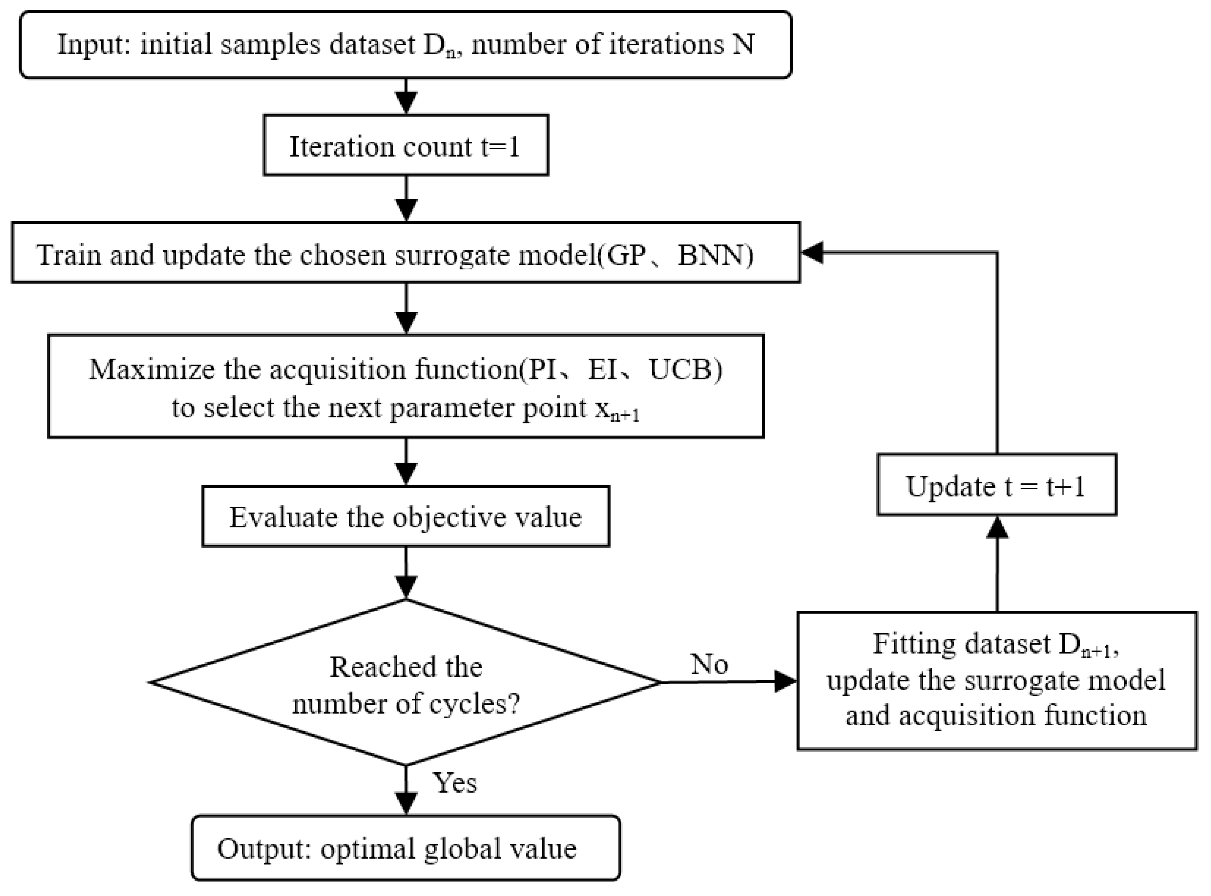
The acquisition function relies on the surrogate model to provide an efficient, intelligent, and active search for the optimal target. It is constructed based on the posterior probability distribution $P\left(H\right|D)$ and determines the next most “potential” evaluation point by maximizing the acquisition function. A suitable acquisition function can effectively ensure the minimum total loss and maintain a balance between exploitation (i.e., using the currently developed area to search for predictions around the optimal value) and exploration (the unknown area where the uncertainty is high). This section briefly introduces the acquisition functions PI, EI, and UCB. For details, see Supplementary Materials.

Probability of Improvement (PI)

$$PI\left(x\right)=\Phi \left(\frac{u\left(x\right)-f\left(x^{+}\right)-\xi }{\sigma \left(x\right)}\right)$$

(4)

where $\Phi (\cdot )$ represents the cumulative probability distribution (CDF); $f\left(x^{+}\right)$ represents the best value among all parameter combinations tested so far; $x^{+}$ represents the best parameter combination itself; $\xi$ is a minimal positive integer. A threshold is set above the current optimal value (see Equation (4)).

Expected Improvement (EI)

$$\begin{gathered} EI\left(x\right)=\left\{\begin{array}{c}\left({\mu }_t\left(x\right)-f\left(x^{+}\right)-\xi \right)\Phi \left(Z\right)+{\sigma }_t\left(x\right)\phi \left(Z\right), if {\sigma }_t\left(x\right)>0\\ 0, if {\sigma }_t\left(x\right)=0\end{array}\right. \\ Z=\frac{{\mu }_t\left(x\right)-f\left(x^{+}\right)-\xi }{{\sigma }_t\left(x\right)} \end{gathered}$$

(5)

where $\Phi (·)$ and $\phi (·)$ are the cumulative distribution function (CDF) and the probability density function (PDF) of the standard normal distribution [36], respectively; $\xi$ is a parameter, which is used to balance exploration and development; $f\left(x^{+}\right)$ is the current maximum; $x^{+}={argmax}_{x_i\in x_{1:t}}f\left(x_i\right)$, where $x_i$ is the query position of the i-th step (see Equation (5)).

Upper Confidence Bound (UCB)

$$UCB\left(x;D\right)=\mu \left(x\right)+\beta \sigma \left(x\right)$$

(6)

For any $x$ in the dataset $D$, the first item is the mean $\mu \left(x\right)$, focusing on development; the second item has a standard deviation $\sigma \left(x\right)$, which reflects the floating range and degree; $\beta$ is often the Chernoff–Hoeffding bound [37]; the larger $\beta$ is, the more emphasis is placed on exploration (see Equation (6)).

2.1.4. Algorithm

BO framework for CO₂ photocatalytic reduction:

Input: a dataset consisting of n initial samples D_n, set the number of iterations N

Output: the global optimal value for the desired properties (the yield or selectivity of CH₄)

(1)

Begin with t = 1;

(2)

Pre-sample, build initial samples [38], train and update the chosen surrogate model $\widehat{f}\left(x_n\right)$, $x_n\in \mathrm{X}$;

(3)

For i = 1, 2,..., measure the CO₂ photocatalytic properties $f\left(x_n\right)$ represented by known parameter values [39] (partial pressure $P_i$ and/or deactivation time h) $x_n$;

(4)

Maximize the acquisition function $A\left(x_n\right)$ to determine the next evaluated process parameter value $x_{n+1}$: $x_{n+1}={\mathit{\text{argmax}}}_{xϵX}A\left(x|D_{1:n}\right)$;

(5)

Evaluate the objective function value $f\left(x_{n+1}\right)=\widehat{f}\left(x_{n+1}\right)+{\epsilon }_{n+1}$;

(6)

Fitting data: $D_{n+1}=D_n\cup \left(x_{n+1},f\left(x_{n+1}\right)\right)$, update the probability surrogate model;

(7)

Update t = t + 1;

(8)

BO actively iterates increases from t times to N times in the feedback loop until it finds the optimal global value $x^{\mathrm{*}}$ (see Equation (7)).

$$\begin{array}{c}{x}^{\mathrm{*}}= \mathit{\text{argmax}} f\left(x\right)\\ x\in X_n\end{array}$$

(7)

$$\begin{array}{c} \hspace{1em}\hspace{1em}{x}_{n+1}= \mathit{\text{argmax}} A\left(x;{\widehat{f}}_n\left(x\right)\right)\\ x\in X\end{array}$$

(8)

2.1.5. Design of Experiments (DOE)

The basic principles of DOE are repetition, randomization, and chunking, which means allowing for repetition of basic experiments, random determination of the order of each experiment, chunking of the search space, and enabling internal comparison of experimental conditions of interest. This paper uses doepy (https://pypi.org/project/doepy/ (accessed on 16 February 2023)), a third-party extension package for Python, to implement the DOE sampling method, using three main sampling methods, URS, LHS, and OLHS.

Latin hypercube sampling (LHS), a stratified random sampling, enables efficient sampling from intervals of the distribution of variables. Assuming that there are k variables x₁, x₂ … x_k, to take N samples from their specified intervals, the cumulative distribution of each variable is divided into the same N small intervals, and a value is randomly selected from each interval. The N values of each variable are randomly combined with the values of the other variables. Unlike random sampling, this method can guarantee total coverage of each range of variables by maximizing the stratification of each marginal distribution.

Uniform random sampling (URS). This module generates uniformly distributed random numbers at intervals you specify. The same non-negative seeds and parameters generate random numbers and then generate a normal distribution. The seeds are reset to the specified value each time a repeatable sequence is started. The general method uses the inverse transform sampling method of the target random variable’s cumulative distribution function (CDF). Because simulations using this method require reversing the CDF of the target variable, alternative methods have been devised for cases where the CDF is not in closed form.

Optimal Latin hypercube sampling (OLHS), which optimizes the sampling process by using the ESE algorithm [40] based on LHS, aims to make the (generalized) distance between sample points larger so that the sample points are entirely scattered in the overall design space. It is worth noting that the values of x and y did not change during the entire optimization process, but the distribution of sample points was changed by using different combinations. Using a matrix operation for high-dimensional problems can significantly speed up the optimization process. Meanwhile, there are mature theoretical and experimental results for the algorithm’s parameters, such as threshold values.

2.1.6. Langmuir–Hinshelwood (L-H) Mechanism

The L-H mechanism is a heterogeneous catalytic mechanism in which the surface reaction is controlled by two adsorbed molecules [41]. The two reactants (CO₂ and H₂O) are first adsorbed onto the solid catalyst; the redox reaction takes place on the surface, and then the products are desorbed again. The surface reaction is the rate-controlling step, as the adsorption and desorption rates are much higher than the surface reaction rates [2]. As can be seen from the kinetic model, the process parameters that affect the rate of CO₂ reduction include the constant rate $k$, irradiance $I$, light intensity $\alpha$, equilibrium adsorption constant $K_i$, partial pressure $P_i$, non-uniform coefficient of reactants $n$, all reactants and product $z$. In addition, temperature, photocatalyst, and photoreactor are also factors that affect the rate of CO₂ photoreduction. According to a related paper [42], the rate constant $k$ and the equilibrium adsorption constant $K_i$ can be determined based on experimental results of CO₂ photoreduction with a specific photocatalyst at a specific temperature T, irradiance $I$, and light intensity $\alpha$.

2.2. Kinetic Models

2.2.1. L-H-Based Kinetic Model

For CO₂ photoreduction, the rate expression must consider the light intensity ($I$) because the reaction occurs at the active site of the light. Since the complete mechanism and activation steps are still unknown, an empirically derived kinetic model of CO₂ photoreduction provides an alternative to the microkinetic modeling approach, whose model expression is shown in Equation (9).

$$r=k{I}^{\alpha }\frac{{\prod }_{i=1}^n{K}_i{P}_i}{{\left(1+{\sum }_{i=1}^z{K}_i{P}_i\right)}^n}$$

(9)

Parameter annotation:

$r$: CO₂ reduction reaction rate ($\mathsf{\mu }\mathrm{m}\mathrm{o}\mathrm{l}·{\mathrm{g}}_{\mathrm{c}\mathrm{a}\mathrm{t}}^{-1}·{\mathrm{h}}^{-1}$)

$k$: Rate constant ($\mathsf{\mu }\mathrm{m}\mathrm{o}\mathrm{l}·{\mathrm{g}}_{\mathrm{c}\mathrm{a}\mathrm{t}}^{-1}·{\mathrm{h}}^{-1}$); the value of $k$ is only a function of temperature (T)

$I$: Irradiance ($\mathrm{m}\mathrm{w}/{\mathrm{c}\mathrm{m}}^2$); depends on the geometry of the photoreactor

$\alpha$: Reaction order of light intensity

$K_i$: Equilibrium adsorption constants for reactants and products (${\mathrm{b}\mathrm{a}\mathrm{r}}^{-1}$)

$P_i$: Partial pressure of reactants and products ($\mathrm{b}\mathrm{a}\mathrm{r}$)

$n$: The inhomogeneity coefficient of adsorbed reactants in elementary surface reactions indicates the magnitude of the effect of concentration on the reaction rate

$z$: Quantities of all reactants and products.

2.2.2. A Probabilistic L-H-Based Dynamic Kinetic Model

The illuminated area ($\mathsf{\mu }\mathrm{m}\mathrm{o}\mathrm{l}{\mathrm{c}\mathrm{m}}^{-2}{\mathrm{h}}^{-1}$) is used to develop a kinetic model scalable relative to light rather than the mass of the photocatalyst. A new model is introduced that can be scaled for light (flexibility), for describing the change in the photocatalyst over time, and for attempting to include only the active sites involved; the estimated coverage is used to calculate the kinetic data rate (see Equation (10)).

$$r=k\frac{I^{\alpha }}{{\eta }_d}{\left(\frac{t}{{\eta }_d}\right)}^{I^{\alpha }-1}{{exp}^{-\left(\frac{t}{{\eta }_d}\right)}}^{I^{\alpha }}\frac{{\prod }_{i=1}^n{{(K}_i{P}_i)}^{ai}}{{\left(1+{\sum }_{i=1}^z{K}_i{P}_i\right)}^{\sum ai}}$$

(10)

Parameter annotation:

$r$: CO₂ reduction reaction rate ($\mathsf{\mu }\mathrm{m}\mathrm{o}\mathrm{l}{\mathrm{c}\mathrm{m}}^{-2}{\mathrm{h}}^{-1}$)

$k$: Rate constant ($\mathsf{\mu }\mathrm{m}\mathrm{o}\mathrm{l}{\mathrm{c}\mathrm{m}}^{-2}{\mathrm{h}}^{-1}$)

$t$: Time ($\mathrm{h}$)

$I$: $I=\frac{I}{I_0}$, Irradiance (dimensionless)

$\alpha$: Reaction order of light intensity (dimensionless)

${\eta }_d$: The deactivation scale parameter (dimensionless)

$K_i$: Equilibrium adsorption constants for reactants and products (${\mathrm{b}\mathrm{a}\mathrm{r}}^{-1}$)

$P_i$: Partial pressure of reactants and products ($\mathrm{b}\mathrm{a}\mathrm{r}$)

$n$: The inhomogeneity coefficient of adsorbed reactants in elementary surface reactions indicates the magnitude of the effect of concentration on the reaction rate

$ai$: The number of moles for each reactant from the assumed surface reaction

$z$: Quantities of all reactants and products.

2.3. CO₂ Photoreduction Kinetic Model

2.3.1. Tan

Tan et al. [2] systematically studied the process parameters; the irradiance $I$ is 81 $\mathrm{m}\mathrm{w}/{\mathrm{c}\mathrm{m}}^2$, the light intensity $\alpha$ is 0.044, the reaction rate constant $k$ was determined to be 84.42 $\mathsf{\mu }\mathrm{m}\mathrm{o}\mathrm{l}·{\mathrm{g}}_{\mathrm{c}\mathrm{a}\mathrm{t}}^{-1}·{\mathrm{h}}^{-1}$, and the adsorption equilibrium constants $K_{C{O}_2} \mathrm{a}\mathrm{n}\mathrm{d} K_{H_{2}O}$ are 0.019${\mathrm{b}\mathrm{a}\mathrm{r}}^{-1}$ and 8.07 ${\mathrm{b}\mathrm{a}\mathrm{r}}^{-1}$, respectively. Combining the values of the determined kinetic constants, the kinetic model of the photocatalytic reduction of CO₂ on 5GO-OTiO₂ is obtained as Equation (11).

$$r=15.953\frac{P_{H_{2}O}{P}_{C{O}_2}}{{\left(1+8.070P_{H_{2}O}+0.0193P_{C{O}_2}\right)}^2}$$

(11)

2.3.2. Khalilzadeh

Khalilzadeh et al. [3] used a doped photocatalyst (Fe-N-Ti@50CPO), and the kinetic model was changed to Equation (12). The kinetic model constants predicted using experimental data for the multi-component system at an irradiance of 85 $\mathrm{m}\mathrm{w}/{\mathrm{c}\mathrm{m}}^2$ and a light intensity $\alpha$ of 0.71 was a reaction rate constant $k$ of 8.33 $\mathsf{\mu }\mathrm{m}\mathrm{o}\mathrm{l}·{\mathrm{g}}_{\mathrm{c}\mathrm{a}\mathrm{t}}^{-1}·{\mathrm{h}}^{-1}$, and the optimum equilibrium rate constants $K_{C{O}_2}$ and $K_{H_{2}O}$ were determined to be 234.31 ${\mathrm{bar}}^{-1}$ and 2091.1${\mathrm{b}\mathrm{a}\mathrm{r}}^{-1}$, respectively, with a non-uniformity factor $n$ of 1.67. Combined with the predicted values of the kinetic constants, the kinetic model of the photocatalytic reduction of CO₂ on Fe-N-Ti@50CPO is shown in Equation (13).

$$r=k{I}^{\alpha }\frac{{\left(K_{CO2}{P}_{CO2}\right)}^{\frac{1}{n}}{\left(K_{H2O}{P}_{H2O}\right)}^{\frac{1}{n}}}{{\left(1+{\left(K_{CO2}{P}_{CO2}\right)}^{\frac{1}{n}}+{\left(K_{H2O}{P}_{H2O}\right)}^{\frac{1}{n}}\right)}^2}$$

(12)

$$r=498589.34\frac{{\left(P_{C{O}_2}{P}_{H_{2}O}\right)}^{0.5988}}{{\left(1+{26.24P_{C{O}_2}}^{0.5988}+{97.33P_{H_{2}O}}^{0.5988}\right)}^2}$$

(13)

2.3.3. Thompson

Thompson et al. [5] used the Weibull PDF (probability density function) to describe the deactivation of the catalyst over time in a kinetic model. This function incorporates the parameter ${\eta }_d$ for the change in yield over time and the parameter $\beta$ ($\beta$ = $I^{\alpha }$) for the reduction and deactivation of the active site over time, as in Equation 14. A probabilistic LH-based kinetic model of the assumed product was adopted (see Equation (15)). In particular; the constant irradiance I is 400 $\mathrm{m}\mathrm{w}/{\mathrm{c}\mathrm{m}}^2$; the estimated reaction rate constant $k$ for the CH₄ product was 7.16 × 10⁻¹ $\mathsf{\mu }\mathrm{m}\mathrm{o}\mathrm{l}{\mathrm{c}\mathrm{m}}^{-2}{\mathrm{h}}^{-1}$; the light intensity $\alpha$ and the deactivation scale parameter ${\eta }_d$ were 7.37 × 10⁻² and 4.81, respectively; the equilibrium rate constants $K_{C{O}_2}$ and $K_{H_{2}O}$ were determined to be 3.21 ${\mathrm{b}\mathrm{a}\mathrm{r}}^{-1}$ and 99.99 ${\mathrm{b}\mathrm{a}\mathrm{r}}^{-1}$; and the model coefficients for the other two products are not repeated. Combining the predicted values of the kinetic constants, a probabilistic L-H-based kinetic model is shown in Equation (16). In addition, a model for the selectivity concerning the CH₄ product is shown in Equation (17).

$$PDF(t)=\frac{I^{\alpha }}{{\eta }_d}{\left(\frac{t}{{\eta }_d}\right)}^{I^{\alpha }-1}{{exp}^{-\left(\frac{t}{{\eta }_d}\right)}}^{I^{\alpha }}$$

(14)

$$\left\{\begin{array}{c}{r}_{{CH}_4}=kPDF(t)\frac{{\left(K_{H_{2}O}{P}_{H_{2}O}\right)}^4{K}_{{CO}_2}{P}_{{CO}_2}}{{\left(1+K_{H_{2}O}{P}_{H_{2}O}+K_{{CO}_2}{P}_{{CO}_2}\right)}^5}\\ r_{CO}=kPDF(t)\frac{K_{H_{2}O}{P}_{H_{2}O}{K}_{{CO}_2}{P}_{{CO}_2}}{{\left(1+K_{H_{2}O}{P}_{H_{2}O}+K_{{CO}_2}{P}_{{CO}_2}\right)}^2}\\ r_{H_2}=kPDF(t)\frac{{\left(K_{H_{2}O}{P}_{H_{2}O}\right)}^2}{{\left(1+K_{H_{2}O}{P}_{H_{2}O}+K_{{CO}_2}{P}_{{CO}_2}\right)}^2}\end{array}\right.$$

(15)

$$\left\{\begin{array}{c}{r}_{{CH}_4}=74281779.8584{\left(\frac{t}{4.81}\right)}^{0.5549}{{exp}^{-\left(\frac{t}{4.81}\right)}}^{1.5549}\frac{{P_{H_{2}O}}^4{P}_{{CO}_2}}{{\left(1+99.99P_{H_{2}O}+3.21P_{{CO}_2}\right)}^5}\\ r_{CO}=51.74855{\left(\frac{t}{19.8}\right)}^{0.2339}{{exp}^{-\left(\frac{t}{19.8}\right)}}^{1.2339}\frac{P_{H_{2}O}{P}_{{CO}_2}}{{\left(1+79.33P_{H_{2}O}+22.65P_{{CO}_2}\right)}^2}\\ r_{H_2}=138.93623{\left(\frac{t}{2.78}\right)}^{0.8867}{{exp}^{-\left(\frac{t}{2.78}\right)}}^{1.8867}\frac{{P_{H_{2}O}}^2}{{\left(1+77.22P_{H_{2}O}+12.54P_{{CO}_2}\right)}^2}\end{array}\right.$$

(16)

$${Selectivity}_{{CH}_4}=\frac{r_{{CH}_4}}{r_{CO}+r_{H_2}}$$

(17)

3. Results

Photocatalytic reduction of CO₂ into CH₄ is a prevalent research focus for CO₂ reduction. In this study, three different photocatalytic systems, Tan [2], Khalilzadeh [3], and Thompson [5], were selected to demonstrate the feasibility of performing BO on heterogeneous photocatalysis. The kinetic models of the three systems (

Table 1. Kinetic model name and chemical principle.

Kinetic Model Name	Catalyst	Catalyst Shape	Reaction Time (h)	Photoreactor	Type of Light Source
Tan [2]	5GO-OTiO2	Yellowish solid powder, binary nanocomposites, hybrid heterostructures	8	Continuous gas flow reactor	Xenon arc lamp
Khalilzadeh [3]	0.12%Fe-0.5%N/ TiO2	Nanoparticles, crystal structure	1	Pyrex vessel and quartz tube	70W mercury lamp
Thompson [5]	P25 TiO2	Coating method, pure and cracks, similar coverage	5	Photo differential photoreactor	OmniCure S2000

), built upon the L-H mechanism [43], were used to simulate experimental data under certain reaction conditions (Figure 1). The study began with the Tan and Khalilzadeh systems that had the partial pressure of CO₂ and H₂O as decision variables. The optimization performance of conventional DOE approaches and BO were compared based on the optimized reaction rates. Also, the BO model was further improved by selecting the best combination of different surrogate models and acquisition functions. Finally, the BO optimization of the Thompson system for the selectivity of CH₄ was explored with an additional variable of catalyst deactivation time.

As is shown in Figure 2, BO in this study uses batch data D_n from previous experiments to train the surrogate model, and the acquisition function recommends the next set of experiments by evaluating the prediction results. The iteration continues for N times in the feedback loop until a satisfactory optimal value is found. A detailed introduction of BO and DOE algorithms, as well as the kinetic models of the photocatalytic systems, were included in the “methods and models” section.

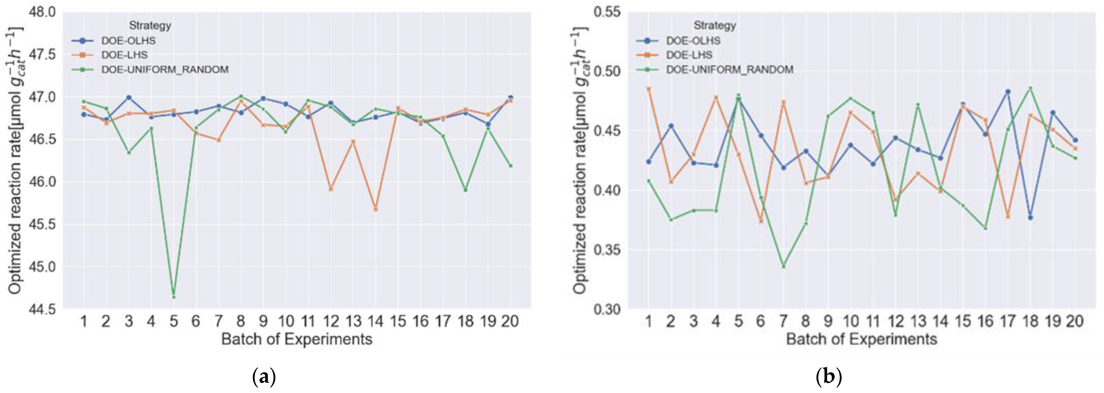
3.1. Comparing Different Traditional DOE Methods in Two-Dimensional Space

First of all, the optimized performance of three DOE methods, optimal Latin hypercube sampling (OLHS [44]), Latin hypercube sampling (LHS [45]), and uniform random sampling (URS [46]), was evaluated on the Tan and Khalilzadeh photocatalysis systems with the partial pressure of H₂O and CO₂ as decision variables. Figure 3 shows that, although the average optimized reaction rates given by the three algorithms are similar, OLHS has the highest stability, while the other two methods have a higher fluctuation of optimized reaction rates between different trials, especially the URS strategy where the biggest difference between the highest and lowest optimized reaction rates reached 0.15 $\mathsf{\mu }\mathrm{m}\mathrm{o}\mathrm{l}·{\mathrm{g}}_{\mathrm{c}\mathrm{a}\mathrm{t}}^{-1}·{\mathrm{h}}^{-1}$ in Tan and 2.364 $\mathsf{\mu }\mathrm{m}\mathrm{o}\mathrm{l}·{\mathrm{g}}_{\mathrm{c}\mathrm{a}\mathrm{t}}^{-1}·{\mathrm{h}}^{-1}$ in Khalilzadeh. The best performance of OLHS was due to the fact that OLHS was optimized on top of LHS in combination with the enhanced stochastic evolutionary (ESE [40]) sampling optimization algorithm. Maximizing the sampling distance in space makes the overall sampling space more homogeneous. In contrast, URS is relatively more random [47].

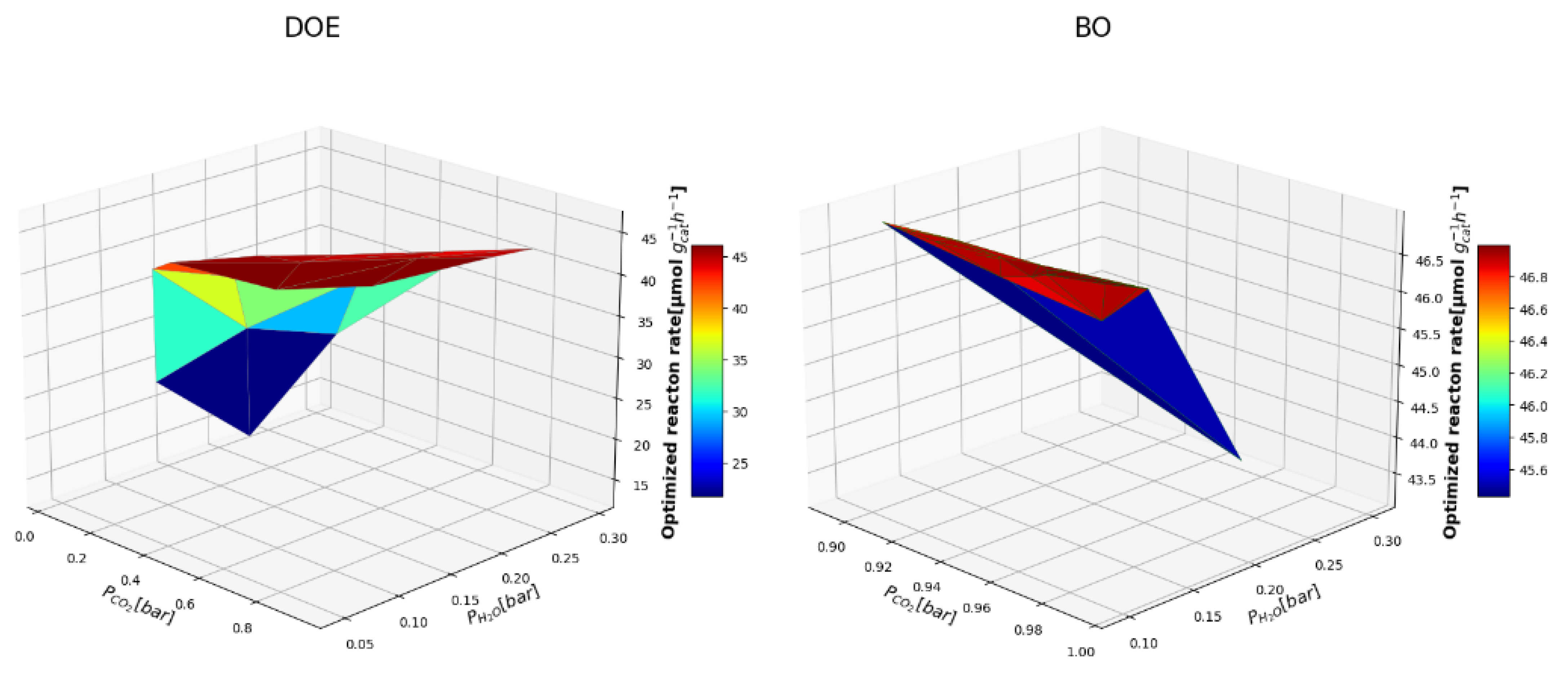
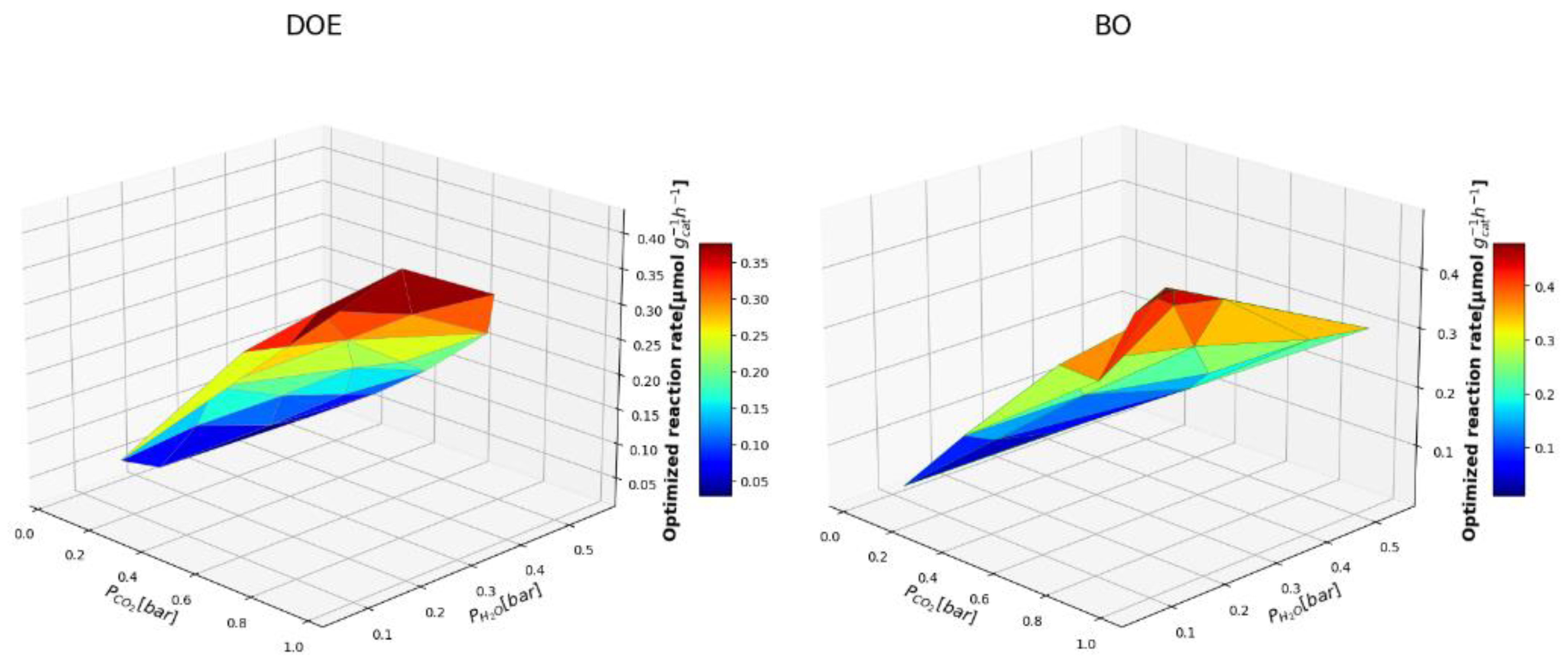
3.2. Comparing BO and DOE-OLHS

The same systems in 3.1 were optimized using BO, and the results are shown in Figure 3. In both the Khalilzadeh and Tan photocatalytic systems, the optimized reaction rates from the BO approach were generally higher than those from the DOE-OLHS, with the maximum optimized reaction rates obtained of 47.339 $\mathsf{\mu }\mathrm{m}\mathrm{o}\mathrm{l}·{\mathrm{g}}_{\mathrm{c}\mathrm{a}\mathrm{t}}^{-1}·{\mathrm{h}}^{-1}$ and 0.490 $\mathsf{\mu }\mathrm{m}\mathrm{o}\mathrm{l}·{\mathrm{g}}_{\mathrm{c}\mathrm{a}\mathrm{t}}^{-1}·{\mathrm{h}}^{-1}$, respectively, which were on average 0.7% and 11.0% higher, respectively, than DOE-OLHS, and on average 1.9% and 13.6% higher, respectively, than the original experimental data. (The optimal partial pressures of CO₂ and H₂O are 0.6 bar and 0.12 bar (Khalilzadeh), and 0.9 bar and 0.173 bar (Tan), respectively.) Meanwhile, the BO method was more stable in the Tan system (Figure 4b), with a difference of only an 1.124% error between the highest and lowest optimized reaction rates, compared to 1.875% in the Khalilzadeh system, which was related to the magnitude difference in the optimized reaction rates between the two systems.

The optimization results of BO and DOE-OLHS were further compared in a 3D triangular surface plot (Figure 5 and Figure 6). The results show that the optimal global solution searched using BO outperforms DOE-OLHS for the same photocatalytic system. During the iterative phase, the data sampled by BO are significantly more compact than those sampled by DOE, as there is a general tendency for the data points sampled by the BO iteration to converge toward the final best point. In contrast, the data points obtained by the DOE-OLHS iteration are more dispersed. In addition, the best reaction rates obtained by BO were higher than those obtained by DOE-OLHS, as is shown in Figure 4.

In this case, the BO strategy, giving the search range for each factor and recommending a more appropriate sampling order based on the distribution of sampling points, exhibited significantly better optimization performance compared to the DOE-OLHS method, which uses a sampling approach in multi-factor search space optimization. Compared to BO’s active learning strategy, DOE’s fixed sampling model tends to lose some of the maximum potential gain points, and it cannot make sampling decisions based on previously obtained experimental data or compromise between exploration and exploration of the search space.

In addition, we assessed the impact of the initial sampling size on BO. The initial sampling size was reduced to five, and the same experiments as in Figure 5 and Figure 6 were performed (Figure S2). The results using 10 initial sampling data had a more concentrated data distribution and obtained a higher optimum response rate than those using 5 initial sampling data. These results suggest that increasing the initial amount of data without increasing the fixed search domain density can significantly improve the performance of BO due to the robustness of GP to non-linear function optimization.

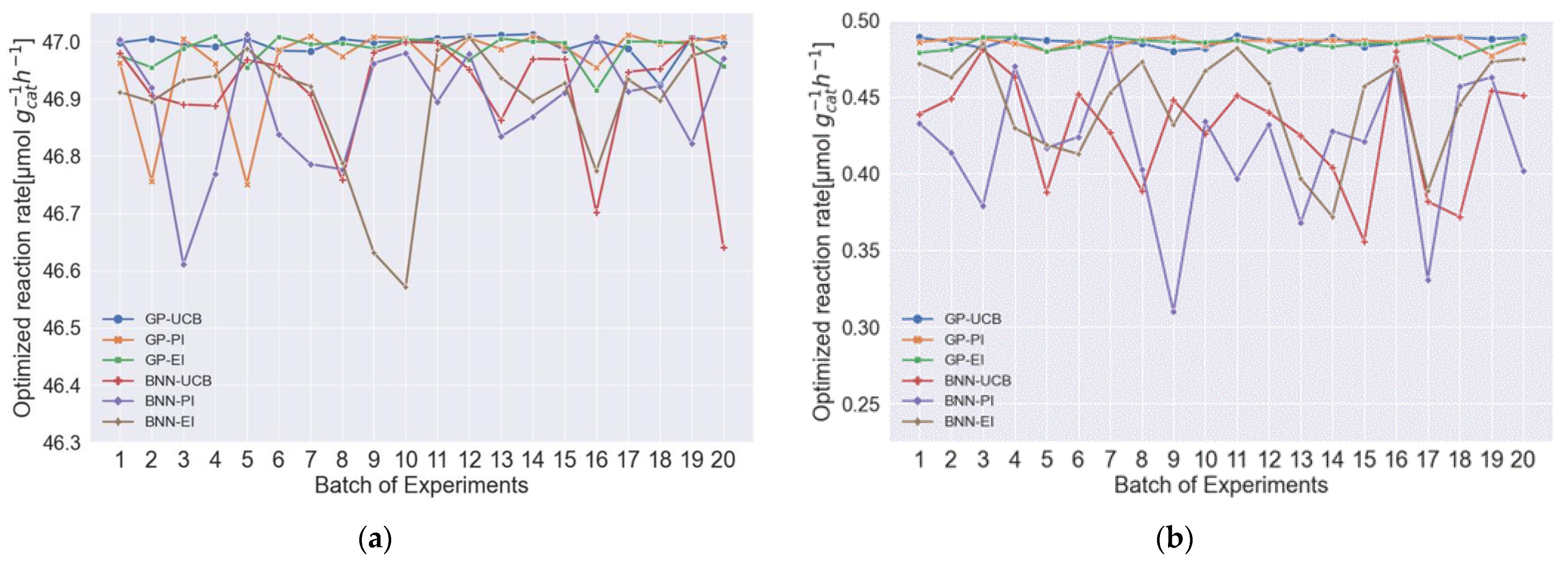
3.3. Investigating the Effects of Different Combinations of Surrogate Models and Acquisition Functions

We also compared the performance of different BO strategies by testing different combinations of surrogate models and acquisition functions. Figure 7 shows that the Gaussian processes (GP) model outperforms the Bayesian neural network (BNN) as the surrogate model, as the combinations with GP reached higher optimized reaction rates. In particular, the combination of GP and upper confidence bound (UCB) had the highest maximum yield and the best stability. In contrast, BNN-EI and BNN-PI yielded the worst optimization in each system. The above results show that GP has better scalability and search performance than BNN in the multi-parameter optimization of both photocatalytic systems. This is because GP’s inherent Gaussian structure allows for fewer parameters to be adjusted compared to BNN, making it suitable for interpretable uncertainty estimation on relatively small data sizes [48], while BNN maximizes performance on various machine-learning tasks with significantly larger datasets [49].

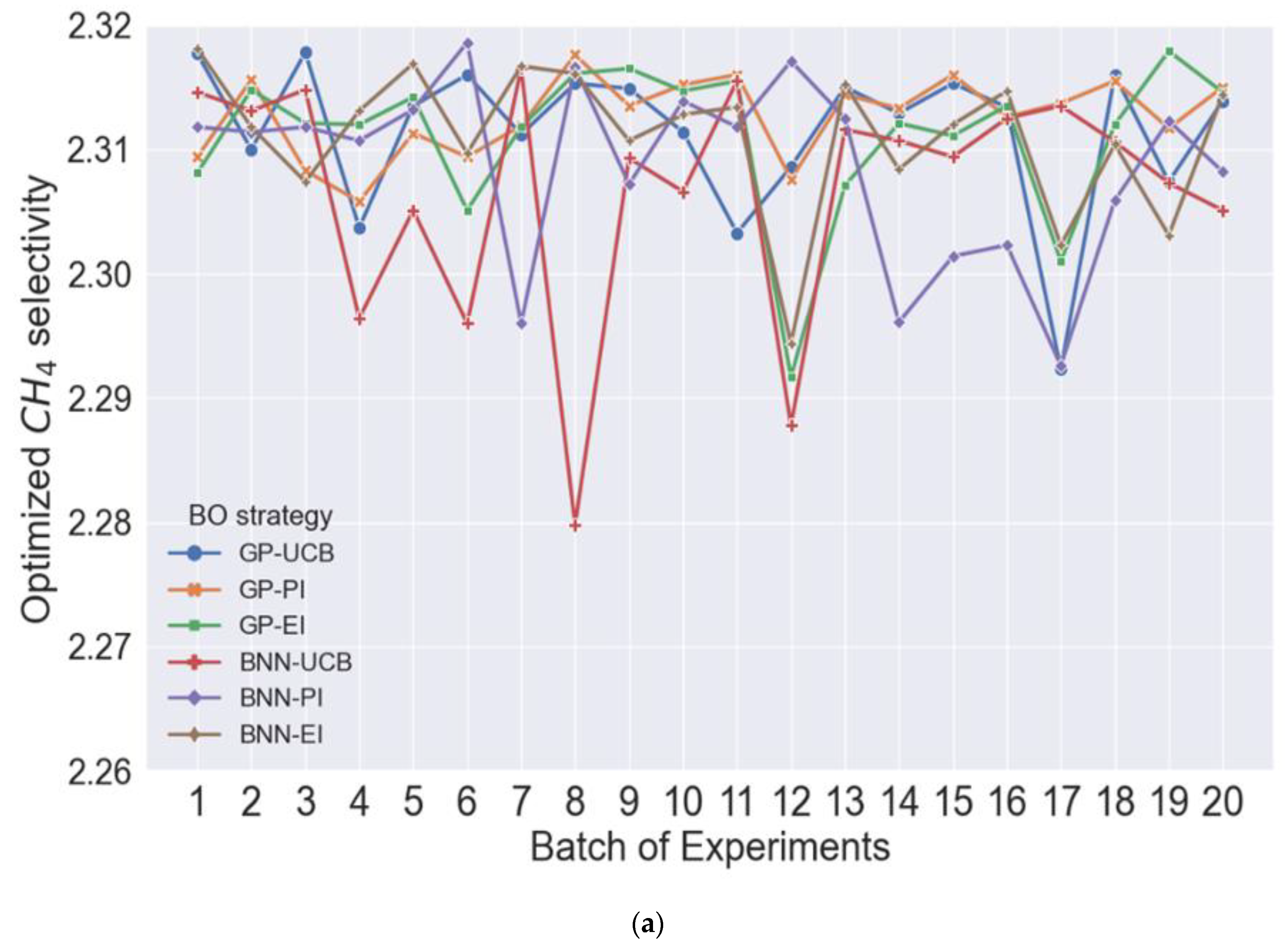
3.4. Optimization of Product Selectivity including Catalyst Deactivation

Thompson’s system with reaction time (t) as an additional variable was optimized by different BO models for the selectivity of CH₄ (Figure 8a). The combination of GP and PI shows the most stable performance with a difference between the highest and lowest optimized selectivity of only 0.012. Therefore, we demonstrated the results of the GP-PI model in a three-dimensional triangular surface plot (Figure 8b). The results show that when the partial pressure of CO₂ is 94.53 kPa, the partial pressure of H₂O is 5.17 kPa, and the time is 2.58 h, the BO model can obtain the best CH₄ selectivity of 2.3176, which is merely 0.1% compared with the corresponding error in the actual experiment. To obtain the maximum CH₄ selectivity of 2.32, the reaction needs to be stopped at a partial pressure of CO₂ of 98.38 kPa and a partial pressure of H₂O of 5.44 kPa for 2.69 h.

On the other hand, the optimized BNN-PI strategy produced the maximum product selectivity of 2.3186 when the partial pressure of CO₂ was 96.23 kPa, the partial pressure of H₂O was 5.34 kPa, and the time was 2.68 h. This is consistent with the increase in sample datasets to enhance the BNN optimization performance mentioned earlier. The previous optimization of reaction rate used a dataset containing 600 samples; here, the product selective optimization uses a dataset containing 1200 samples. In particular, in such a complex product selectivity model, the PI acquisition function tended to explore near the maximum value, which provided a practical compromise for the optimization properties of BNN. To obtain better optimization performance, BNN’s complex model architecture [50] requires more datasets with more samples and more training rounds to demonstrate its powerful learning ability. Overall, the GP surrogate model performs more consistently compared to BNN in bivariate optimization due to GP’s superior performance on small datasets. In contrast, BNN as an inverse optimization method [51] lacks robustness on static datasets compared to the forward optimization of the GP method, which makes it perform better on complex product selectivity models with deactivation times. However, in future research, we expect BNN to perform even better on large mixed dynamic datasets [52].

4. Discussion

For complex and unknown photocatalytic reduction reactions, kinetic models are usually constructed from the rate law developed by the photocatalytic reduction reaction mechanism proposed [53], and the kinetic data are generally estimated using mathematical software methods (such as the least squares regression method) to correlate the input and output data of the photocatalytic reaction experiment [54]. However, kinetic models often assume that the output of the photocatalytic system is only related to the current input and is not affected by the past and future input values and the internal effects of the system (such as feedback mechanisms and nonlinear effects), so they cannot react and predict the historical effects and future trends of the photocatalytic system. The photocatalytic reduction reaction is time-sensitive, while the kinetic model can only describe the short-term behavior of the system but cannot predict its long-term evolution trend. In addition, due to the nonlinear changes in the photocatalytic system, the parameters of the kinetic model may have complex spatial distribution characteristics, which makes it difficult to solve the model parameters accurately.

As a tool for developing experimental strategies, DOE is widely used in scientific fields such as quality control and process improvement. However, as a local optimization algorithm, DOE cannot locate the global optimal solution in the dynamic photocatalytic reduction reaction. In the case of a given range of parameters, DOE has design limitations that involve only three levels [14] and three factors [55]. When there are multi-factor variables or even mixed-parameter spaces containing categorical variables, DOE must carry out factor screening [56], thus increasing the experimental budget. The cost of these experiments is often high for photocatalytic reduction reactions, so the DOE method may not be an ideal method for the optimization of photocatalytic reduction reactions.

BO is a statistics-based optimization algorithm developed to find the global optimal solution to an expensive black-box function. The core components of BO are the surrogate model and acquisition function. The surrogate model is responsible for training the initial dataset fitted from the historical input experimental data; it also makes predictions for the unevaluated simulation experiments to include the effects of past and future inputs on the system. The acquisition function verifies the prediction results of the model mainly by balancing development (known areas with good prediction performance of the model) and exploration (areas with high uncertainty of the unknown) and recommends the next sampling point for testing, which avoids the appearance of locally optimal solutions to a great extent and increases the scientific insights of the system.

We acknowledge that the comparison of various optimization techniques in this study relies on experimental data from kinetic model simulations and is not exceptional compared to earlier results on optimizing photocatalytic CO₂ reduction. The previous experimental optimization [57,58], utilizing the single-variable control approach, displayed encouraging outcomes for both CH₄ yield and selectivity. For instance, Alkanad et al. [57] achieved a methane yield of 48 $\mathsf{\mu }\mathrm{m}\mathrm{o}\mathrm{l}·{\mathrm{g}}_{\mathrm{c}\mathrm{a}\mathrm{t}}^{-1}·{\mathrm{h}}^{-1}$ by optimizing the hydrothermal reaction conditions and identified one catalyst that outperformed the other seven in their experimental comparison. Single-variable optimization methods can be costly and time-consuming in terms of experimentation and data production. However, a simulation of experimental noises was added to the implementation of this work. In addition, the use of simulated data makes sure that all comparison tests are based on the same conditions and baseline level. Although BO has its inherent limitations, such as the high cost of surrogate model calculation for updating and the absence of a general acquisition function, we can still narrow these gaps by designing more advanced models and suitable filters in future studies.

5. Conclusions

In this work, we developed a BO framework and applied it to a series of photocatalytic reduction systems. Compared to the conventional DOE approach for maximum CH₄ yield optimization in the two-variable [P_CO2, P_H2O] space, the global optimization of BO outperformed the DOE approach, and the optimized reaction rates found using BO were 0.7% and 11.0% higher, respectively, than the best results of optimization by DOE, and it was significantly better than the original experimental data, which were 1.9% and 13.6% higher, respectively. In addition, the best combination of the two main components of BO, the surrogate model and acquisition function, was investigated, and the combination of GP and UCB was found to have the highest optimization efficiency, obtained at 47.339 $\mathsf{\mu }\mathrm{m}\mathrm{o}\mathrm{l}·{\mathrm{g}}_{\mathrm{c}\mathrm{a}\mathrm{t}}^{-1}·{\mathrm{h}}^{-1}$ and 0.490 $\mathsf{\mu }\mathrm{m}\mathrm{o}\mathrm{l}·{\mathrm{g}}_{\mathrm{c}\mathrm{a}\mathrm{t}}^{-1}·{\mathrm{h}}^{-1}$, respectively. Furthermore, BO was used to optimize the CH₄ product selectivity model in the Thompson system with the additional variable of catalyst deactivation time. The results showed that BO exhibited superior performance, and the optimization results agreed well with the actual experimental data, with an error of less than 5%. In the meantime, BO was found to significantly increase the efficiency of optimization compared to the traditional DOE methods.

Our BO framework can be conveniently applied to complex photocatalytic systems to optimize multivariable reaction processes. The use of BO can also help the development of photocatalysis experiments toward automation. Future research will aim to improve the BO framework for parallel optimization in a more complex search space (i.e., containing categorical variables). In addition, material descriptors will be added to the BO framework to optimize the selection of photocatalysts in CO₂ photoreduction.

References

1. Tahir, M.; Amin, N.S. Indium-doped TiO2 nanoparticles for photocatalytic CO2 reduction with H2O vapors to CH4. Appl. Catal. B Environ. 2015, 162, 98–109. [Google Scholar] [CrossRef]
2. Tan, L.-L.; Ong, W.-J.; Chai, S.-P.; Mohamed, A.R. Photocatalytic reduction of CO2 with H2O over graphene oxide-supported oxygen-rich TiO2 hybrid photocatalyst under visible light irradiation: Process and kinetic studies. Chem. Eng. J. 2017, 308, 248–255. [Google Scholar] [CrossRef]
3. Khalilzadeh, A.; Shariati, A. Fe-N-TiO2/CPO-Cu-27 nanocomposite for superior CO2 photoreduction performance under visible light irradiation. Solar Energy 2019, 186, 166–174. [Google Scholar] [CrossRef]
4. Sips, R. On the Structure of a Catalyst Surface. J. Chem. Phys. 1948, 16, 490–495. [Google Scholar] [CrossRef]
5. Thompson, W.A.; Sanchez Fernandez, E.; Maroto-Valer, M.M. Probability Langmuir-Hinshelwood based CO2 photoreduction kinetic models. Chem. Eng. J. 2020, 384, 123356. [Google Scholar] [CrossRef]
6. Bu, X.; Xie, G.; Peng, Y.; Chen, Y. Kinetic modeling and optimization of flotation process in a cyclonic microbubble flotation column using composite central design methodology. Int. J. Miner. Process. 2016, 157, 175–183. [Google Scholar] [CrossRef]
7. Danesh, S.M.S.; Faghihian, H.; Shariati, S. Sulfonic Acid Functionalized SBA-3 Silica Mesoporous Magnetite Nanocomposite for Safranin O Dye Removal. Silicon 2018, 11, 1817–1827. [Google Scholar] [CrossRef]
8. Jin, H.; Zhu, J.; Hu, J.; Li, Y.; Zhang, Y.; Huang, X.; Ding, K.; Chen, W. Structural and electronic properties of tungsten trioxides: From cluster to solid surface. Theor. Chem. Acc. 2011, 130, 103–114. [Google Scholar] [CrossRef]
9. Purkait, P.K.; Majumder, S.; Roy, S.; Maitra, S.; Chandra Das, G.; Chaudhuri, M.G. Enhanced heterogeneous photocatalytic degradation of florasulam in aqueous media using green synthesized TiO2 nanoparticle under UV light irradiation. Inorg. Chem. Commun. 2023, 155, 111017. [Google Scholar] [CrossRef]
10. Lais, A.; Gondal, M.A.; Dastageer, M.A.; Al-Adel, F.F. Experimental parameters affecting the photocatalytic reduction performance of CO2 to methanol: A review. Int. J. Energy Res. 2018, 42, 2031–2049. [Google Scholar] [CrossRef]
11. Murray, P.M.; Bellany, F.; Benhamou, L.; Bucar, D.K.; Tabor, A.B.; Sheppard, T.D. The application of design of experiments (DoE) reaction optimisation and solvent selection in the development of new synthetic chemistry. Org. Biomol. Chem. 2016, 14, 2373–2384. [Google Scholar] [CrossRef] [PubMed]
12. Niedz, R.P.; Evens, T.J. Design of experiments (DOE)—History, concepts, and relevance to in vitro culture. Vitr. Cell. Dev. Biol. Plant 2016, 52, 547–562. [Google Scholar] [CrossRef]
13. Lee, B.C.Y.; Mahtab, M.S.; Neo, T.H.; Farooqi, I.H.; Khursheed, A. A comprehensive review of Design of experiment (DOE) for water and wastewater treatment application—Key concepts, methodology and contextualized application. J. Water Process Eng. 2022, 47, 102673. [Google Scholar] [CrossRef]
14. Anika, N.A.; Tanzeem, N.; Gupta, H.S. Design of Experiment (DoE): Implementation in Determining Optimum Design Parameters of Portable Workstation. Engineering 2020, 12, 25–32. [Google Scholar] [CrossRef]
15. Bowden, G.D.; Pichler, B.J.; Maurer, A. A Design of Experiments (DoE) Approach Accelerates the Optimization of Copper-Mediated (18)F-Fluorination Reactions of Arylstannanes. Sci. Rep. 2019, 9, 11370. [Google Scholar] [CrossRef] [PubMed]
16. Lucks, S.; Brunner, H. In Situ Generated Palladium on Aluminum Phosphate as Catalytic System for the Preparation of β,β-Diarylated Olefins by Matsuda–Heck Reaction. Org. Process Res. Dev. 2017, 21, 1835–1842. [Google Scholar] [CrossRef]
17. Caron, S.; Thomson, N.M. Pharmaceutical Process Chemistry: Evolution of a Contemporary Data-Rich Laboratory Environment. J. Org. Chem. 2015, 80, 2943–2958. [Google Scholar] [CrossRef]
18. Emmerich, M.T.M.; Giannakoglou, K.C.; Naujoks, B. Single- and multiobjective evolutionary optimization assisted by Gaussian random field metamodels. IEEE Trans. Evol. Comput. 2006, 10, 421–439. [Google Scholar] [CrossRef]
19. Shuai, D. Hyper parameter optimization of CNN based on improved Bayesian Optimization algorithm. Appl. Res. Comput. 2018, 36, 1984–1987. [Google Scholar] [CrossRef]
20. Rasmussen, C.E. Gaussian Processes in Machine Learning. In Advanced Lectures on Machine Learning, Proceedings of the ML Summer Schools 2003, Canberra, Australia, 2–14 February 2003, Tübingen, Germany, 4–16 August 2003; Revised Lectures; Bousquet, O., von Luxburg, U., Rätsch, G., Eds.; Springer: Berlin/Heidelberg, Germany, 2004; pp. 63–71. [Google Scholar] [CrossRef]
21. Kusner, M.J.; Paige, B.; Hernández-Lobato, J.M. Grammar Variational Autoencoder. Mach. Learn. 2017, 2017, 1945–1954. [Google Scholar] [CrossRef]
22. Cui, J.; Yang, B. Survey on Bayesian optimization methodology and applications. J. Softw. 2018, 29, 3068–3090. (In Chinese) [Google Scholar] [CrossRef]
23. Häse, F.; Roch, L.M.; Kreisbeck, C.; Aspuru-Guzik, A. Phoenics: A Bayesian Optimizer for Chemistry. ACS Cent. Sci. 2018, 4, 1134–1145. [Google Scholar] [CrossRef]
24. Seifrid, M.; Pollice, R.; Aguilar-Granda, A.; Morgan Chan, Z.; Hotta, K.; Ser, C.T.; Vestfrid, J.; Wu, T.C.; Aspuru-Guzik, A. Autonomous Chemical Experiments: Challenges and Perspectives on Establishing a Self-Driving Lab. ACC Chem. Res. 2022, 55, 2454–2466. [Google Scholar] [CrossRef] [PubMed]
25. Shields, B.J.; Stevens, J.; Li, J.; Parasram, M.; Damani, F.; Alvarado, J.I.M.; Janey, J.M.; Adams, R.P.; Doyle, A.G. Bayesian reaction optimization as a tool for chemical synthesis. Nature 2021, 590, 89–96. [Google Scholar] [CrossRef] [PubMed]
26. Christensen, M.; Yunker, L.P.E.; Adedeji, F.; Häse, F.; Roch, L.M.; Gensch, T.; dos Passos Gomes, G.; Zepel, T.; Sigman, M.S.; Aspuru-Guzik, A.; et al. Data-science driven autonomous process optimization. Commun. Chem. 2021, 4, 112. [Google Scholar] [CrossRef]
27. Deshwal, A.; Simon, C.M.; Doppa, J.R. Bayesian optimization of nanoporous materials. Mol. Syst. Des. Eng. 2021, 6, 1066–1086. [Google Scholar] [CrossRef]
28. Taw, E.; Neaton, J.B. Accelerated Discovery of CH4 Uptake Capacity Metal–Organic Frameworks Using Bayesian Optimization. Adv. Theory Simul. 2022, 5, 515. [Google Scholar] [CrossRef]
29. Xie, Y.; Zhang, C.; Deng, H.; Zheng, B.; Su, J.W.; Shutt, K.; Lin, J. Accelerate Synthesis of Metal-Organic Frameworks by a Robotic Platform and Bayesian Optimization. ACS Appl. Mater. Interfaces 2021, 13, 53485–53491. [Google Scholar] [CrossRef]
30. Pang, Y.; Zang, X.; Li, H.; Liu, J.; Chang, Q.; Zhang, S.; Wang, C.; Wang, Z. Solid-phase microextraction of organophosphorous pesticides from food samples with a nitrogen-doped porous carbon derived from g-C3N4 templated MOF as the fiber coating. J. Hazard. Mater. 2020, 384, 121430. [Google Scholar] [CrossRef]
31. Hao, W.; Dit-Yan, Y. A Survey on Bayesian Deep Learning. ACM Comp. Surv. 2020, 53, 1–37. [Google Scholar] [CrossRef]
32. Lei, B.; Kirk, T.Q.; Bhattacharya, A.; Pati, D.; Qian, X.; Arroyave, R.; Mallick, B.K. Bayesian optimization with adaptive surrogate models for automated experimental design. npj Comput. Mater. 2021, 7, 194. [Google Scholar] [CrossRef]
33. Ronquist, F.; Teslenko, M.; van der Mark, P.; Ayres, D.L.; Darling, A.; Hohna, S.; Larget, B.; Liu, L.; Suchard, M.A.; Huelsenbeck, J.P. MrBayes 3.2: Efficient Bayesian Phylogenetic Inference and Model Choice Across a Large Model Space. Syst. Biol. 2012, 61, 539–542. [Google Scholar] [CrossRef] [PubMed]
34. Ma, X.; Blaschko, M.B. Additive Tree-Structured Conditional Parameter Spaces in Bayesian Optimization: A Novel Covariance Function and a Fast Implementation. IEEE Trans. Pattern Anal. Mach. Intell. 2021, 43, 3024–3036. [Google Scholar] [CrossRef] [PubMed]
35. Cheng, Z.; Judith, B.; Hedvig, K.; Stephan, M. Advances in Variational Inference. IEEE Trans. Pattern Anal. Mach. Intell. 2018, 41, 2008–2026. [Google Scholar] [CrossRef]
36. Hutter, F.; Hoos, H.H.; Leyton-Brown, K. Sequential Model-Based Optimization for General Algorithm Configuration. In Lecture Notes in Computer Science; Coello, C.A.C., Ed.; Learning and Intelligent Optimization, LION 2011; Springer: Berlin/Heidelberg, Germany, 2011; Volume 6683. [Google Scholar] [CrossRef]
37. Coley, C.W.; Eyke, N.S.; Jensen, K.F. Autonomous Discovery in the Chemical Sciences Part I: Progress. Angew. Chem. Int. Ed. Engl. 2020, 59, 22858–22893. [Google Scholar] [CrossRef] [PubMed]
38. Lookman, T.; Balachandran, P.V.; Xue, D.; Yuan, R. Active learning in materials science with emphasis on adaptive sampling using uncertainties for targeted design. npj Comput. Mater. 2019, 5, 21. [Google Scholar] [CrossRef]
39. Coley, C.W. Defining and Exploring Chemical Spaces. Trends Chem. 2021, 3, 133–145. [Google Scholar] [CrossRef]
40. Jin, R.; Chen, W.; Sudjianto, A. An efficient algorithm for constructing optimal design of computer experiments. J. Stat. Plan. Inference 2005, 134, 268–287. [Google Scholar] [CrossRef]
41. Wang, Y.; Ma, J.; Wang, X.; Zhang, Z.; Zhao, J.; Yan, J.; Du, Y.; Zhang, H.; Ma, D. Complete CO Oxidation by O2 and H2O over Pt–CeO2−δ/MgO Following Langmuir–Hinshelwood and Mars–van Krevelen Mechanisms, Respectively. ACS Catal. 2021, 11, 11820–11830. [Google Scholar] [CrossRef]
42. Matsubara, Y. Standard Electrode Potentials for the Reduction of CO2 to CO in Acetonitrile–Water Mixtures Determined Using a Generalized Method for Proton-Coupled Electron-Transfer Reactions. ACS Energy Lett. 2017, 2, 1886–1891. [Google Scholar] [CrossRef]
43. Kumar, K.V.; Porkodi, K.; Rocha, F. Langmuir–Hinshelwood kinetics—A theoretical study. Catal. Commun. 2008, 9, 82–84. [Google Scholar] [CrossRef]
44. Pholdee, N.; Bureerat, S. An efficient optimum Latin hypercube sampling technique based on sequencing optimisation using simulated annealing. Int. J. Syst. Sci. 2013, 46, 1780–1789. [Google Scholar] [CrossRef]
45. Ayyub, B.M.; Lai, K.-L. Selective Sampling in Simulation-Based Reliability Assessment. Int. J. Press. Vessel. Pip. 1991, 46, 229–249. [Google Scholar] [CrossRef]
46. Corona, P.; Franceschi, S.; Pisani, C.; Portoghesi, L.; Mattioli, W.; Fattorini, L. Inference on diversity from forest inventories: A review. Biodivers. Conserv. 2015, 26, 3037–3049. [Google Scholar] [CrossRef]
47. Lee, J.-H.; Ko, Y.-D.; Yun, I.-G.; Han, K.-H. Comparison of Latin Hypercube Sampling and Simple Random Sampling Applied to Neural Network Modeling of HfO2 Thin Film Fabrication. Trans. Electr. Electron. Mater. 2006, 7, 210–214. [Google Scholar] [CrossRef]
48. Belkin, M. Fit without fear: Remarkable mathematical phenomena of deep learning through the prism of interpolation. Mach. Learn. 2021, 30, 203–248. [Google Scholar] [CrossRef]
49. Semenova, E.; Williams, D.P.; Afzal, A.M.; Lazic, S.E. A Bayesian neural network for toxicity prediction. Comput. Toxicol. 2020, 16, 100133. [Google Scholar] [CrossRef]
50. Dawson, J.M.; Davis, T.A.; Gomez, E.L.; Schock, J. A self-supervised, physics-aware, Bayesian neural network architecture for modelling galaxy emission-line kinematics. Mon. Not. R. Astron. Soc. 2021, 503, 574–585. [Google Scholar] [CrossRef]
51. Kingma, D.P.; Welling, M. Auto-Encoding Variational Bayes. arXiv 2013, arXiv:1312.6114. [Google Scholar]
52. Häse, F.; Aldeghi, M.; Hickman, R.J.; Roch, L.M.; Aspuru-Guzik, A. Gryffin: An algorithm for Bayesian optimization of categorical variables informed by expert knowledge. Appl. Phys. Rev. 2021, 8, 48164. [Google Scholar] [CrossRef]
53. Abdullah, H.; Khan, M.M.R.; Yaakob, Z.; Ismail, N.A. A kinetic model for the photocatalytic reduction of CO2 to methanol pathways. IOP Conf. Ser. Mater. Sci. Eng. 2019, 702, 012026. [Google Scholar] [CrossRef]
54. Luong, G.K.T.; Ku, Y. Enhanced photocatalytic reduction of Cr(VI) in aqueous solution by UV/TiO2 process in the presence of Fe(III): Performance, kinetic, and mechanisms. Chem. Eng. Process. Process Intensif. 2022, 181, 109135. [Google Scholar] [CrossRef]
55. Liu, T.; Yu, X.; Yin, H. Study of Top-down and Bottom-up Approaches by Using Design of Experiment (DoE) to Produce Meloxicam Nanocrystal Capsules. AAPS PharmSciTech 2020, 21, 79. [Google Scholar] [CrossRef] [PubMed]
56. Vardhan, H.; Mittal, P.; Adena, S.K.; Mishra, B. Long-circulating polyhydroxybutyrate-co-hydroxyvalerate nanoparticles for tumor targeted docetaxel delivery: Formulation, optimization and in vitro characterization. Eur. J. Pharm. Sci. 2017, 99, 85–94. [Google Scholar] [CrossRef] [PubMed]
57. Alkanad, K.; Hezam, A.; Al-Zaqri, N.; Bajiri, M.A.; Alnaggar, G.; Drmosh, Q.A.; Almukhlifi, H.A.; Neratur Krishnappagowda, L. One-Step Hydrothermal Synthesis of Anatase TiO2 Nanotubes for Efficient Photocatalytic CO2 Reduction. ACS Omega 2022, 7, 38686–38699. [Google Scholar] [CrossRef]
58. Deng, H.; Zhu, X.; Chen, Z.; Zhao, k.; Cheng, G. Oxygen vacancy engineering of TiO2-x nanostructures for photocatalytic CO2 reduction. Carbon Lett. 2022, 32, 1671–1680. [Google Scholar] [CrossRef]
Figure 1. Workflow of the BO framework, including combination and optimization.
Processes 11 02614 g001
Figure 2. Bayesian optimization flowchart.
Processes 11 02614 g002
Figure 3. Contains 20 batch tests with 20 experimental sampling points per batch taking the optimal reaction rate for each batch; scatter shapes are used to distinguish between different DOE strategies, and line plots are used to observe the trend of the maximum yield. (a) Khalilzadeh. Multivariate optimization comparison of maximum yields for DOE methods. (b) Tan. Multivariate optimization comparison of DOE methods for maximum yield.
Processes 11 02614 g003
Figure 4. Comparison of BO and DOE for maximum reaction rate optimization in multivariate search space for two photosensitized systems. The BO was initialized with 10 LHS containing 20 batch trials with 20 simulations per batch to take the optimal reaction rate per batch; the DOE was 20 OLHS sampling points; scatter shapes are used to distinguish the different optimization strategies, and line plots are used to observe the trend of the maximum yield. (a) Comparison of multivariate optimization of Khalilzadeh. BO (GP-UCB) with DOE maximum yield. (b) Multivariate optimization comparison of Tan. BO (GP-UCB) with DOE maximum yield.
Processes 11 02614 g004
Figure 5. Comparison of DOE (OLHS) and BO (GP-UCB, 10 LHS samples) binary optimization results in Khalilzadeh. Curved triangulation distinguishes the size and distribution of the data, with triangular colors used to distinguish the magnitude of the values, with the corresponding optimized reaction rate color bars on the right.
Processes 11 02614 g005
Figure 6. Comparison of DOE (OLHS) and BO (GP-UCB, 10 LHS samples) binary optimization results in Tan. Curved triangulation distinguishes the size and distribution of the data, with triangular colors used to distinguish the magnitude of the values, with the corresponding optimized reaction rate color bars on the right.
Processes 11 02614 g006
Figure 7. BO models’ optimization results compare six combinations of surrogate models and acquisition functions under two photocatalytic systems. The BO was initialized with 10 LHS containing 20 batch tests and 20 simulations per batch, and the optimal reaction rate was taken for each batch. The rates were plotted as line plots (a,b), using scatter shapes to distinguish between different BO strategies and lines connecting the scatters to observe the trend in maximum yield. (a) Khalilzadeh. Optimal reaction rate; (b) Tan. Optimal reaction rate.
Processes 11 02614 g007
Figure 8. Comparison of different BO selectivity models for CH4 under the Thompson photocatalytic system. (a) BO strategy screening. The optimization results of BO models for six different combinations of surrogate models and acquisition functions were compared for the selectivity model of CH4. Twenty batches of simulation trials were conducted for each strategy separately; each set of trials was initialized with 10 LHS points for the BO framework and iterated 50 times separately; the optimal reaction rate for each batch was taken to plot the experimental simulation points; scatter shapes are used to distinguish the different BO strategies, and scatter points are connected with a dash to observe the trend of maximum yield; (b) 3D triangular surface plots containing catalyst deactivation times were drawn using the data from the better-performing BO models (BNN-PI and GP-PI) in (a), where the 3D coordinates indicate the partial pressures of CO2 and H2O, and the catalyst deactivation time, respectively. The triangulation of the surface distinguishes the size and distribution of the data, and colors are used to distinguish the magnitude of the values, with the corresponding color bars of the optimized deactivation time to the right.
Processes 11 02614 g008aProcesses 11 02614 g008b