A Timestep-Adaptive-Diffusion-Model-Oriented Unsupervised Detection Method for Fabric Surface Defects

Abstract

Defect detection is crucial in quality control for fabric production. Deep-learning-based unsupervised reconstruction methods have been recognized universally to address the scarcity of fabric defect samples, high costs of labeling, and insufficient prior knowledge. However, these methods are subject to several weaknesses in reconstructing defect images into defect-free images with high quality, like image blurring, defect residue, and texture inconsistency, resulting in false detection and missed detection. Therefore, this article proposes an unsupervised detection method for fabric surface defects oriented to the timestep adaptive diffusion model. Firstly, the Simplex Noise–Denoising Diffusion Probabilistic Model (SN-DDPM) is constructed to recursively optimize the distribution of the posterior latent vector, thus gradually approaching the probability distribution of surface features of the defect-free samples through multiple iterative diffusions. Meanwhile, the timestep adaptive module is utilized to dynamically adjust the optimal timestep, enabling the model to flexibly adapt to different data distributions. During the detection, the SN-DDPM is employed to reconstruct the defect images into defect-free images, and image differentiation, frequency-tuned salient detection (FTSD), and threshold binarization are utilized to segment the defects. The results reveal that compared with the other seven unsupervised detection methods, the proposed method exhibits higher F1 and IoU values, which are increased by at least 5.42% and 7.61%, respectively, demonstrating that the proposed method is effective and accurate.

1. Introduction

Fabric defect detection plays a key role in controlling textile quality. Fabric defects may influence the appearance of the product, resulting in performance degradation or even functional failure. Punctual detection and repair of fabric defects can lower the defective rate and scrapped quantity, reduce waste and repeated production costs, ensure the qualification of final products, and improve customer satisfaction and brand reputation [1]. However, manual detection currently still prevails in many enterprises, which not only places high requirements on the technical qualifications of inspectors but also leads to a heavy burden of labor costs. Consequently, promoting a highly precise and efficient fabric defect detection system is extremely significant in improving product quality, ensuring the smooth running of production machines, and effectively lowering labor costs [2].

Machine vision has been highly recognized and is gradually replacing manual vision, becoming an important application in fabric defect detection. Machine vision detection, a traditional processing method for images, can extract low-level features of images by obtaining prior knowledge of defect features, thus identifying and classifying the defects [3]. Under the premise of ensuring accuracy, machine vision detection can realize automation and intelligence while imposing high requirements for camera performance and light source environment [4]. Fabric defects are diversified in form and complicated in texture, as shown in Figure 1. Notably, small defects, as displayed in Figure 1b, occupy fewer pixels and have little impact on the overall structure or pattern of the image, increasing the difficulty of distinguishing them from the surrounding texture or pattern. Owning to the above factors, machine vision fails to recognize defects in specific textured fabrics, which is only one of its application restrictions.

Deep learning technologies break through the deficiencies of traditional machine learning technologies. The deep-learning-based supervised detection method [5,6], which automatically extracts the features of the detected object, has shown significant effectiveness in image classification, which further supports its application in surface defect detection. Notably, the deep-learning-based supervised detection method possesses high performance but still requires lots of annotated data to train the model and a certain number of defect samples as references. Actually, collecting and annotating numerous defect sample data is challenging and even impractical [7]. Therefore, some scholars [8,9,10] have comprehensively and extensively studied deep-learning-based unsupervised detection methods to detect surface defects. A prevailing method [11,12] is to obtain the reconstruction models with positive product features by learning defect-free samples, then reconstructing defect images into defect-free images by utilizing the trained reconstruction models, and positioning defects by comparing the differences before and after reconstruction.

The above method is superior because it does not require obtaining the defect type in advance and free from labeling of the sample defects. Currently, the unsupervised defect detection models primarily include the generative adversarial network (GAN) [13] and the automatic encoder (AE) [14]. Nevertheless, these models face challenges in reconstructing defect images into defect-free images in a high-quality manner [15], causing lower accuracy in defect detection. GAN is composed of manually designed generators and discriminators and focuses on solving potential gradient vanishing or explosions, increasing its training difficulty. AE maps high-dimensional feature images to low-dimensional vector representations, which leads to pixel merging, resulting in blurry reconstructed images. In addition, the fabric surface texture features are distributed in a non-periodic manner, and such decentralized data are extremely likely to generate a highly similar image to the original one, resulting in residual defects in the reconstructed image. During the post-processing, the fixed threshold segmentation makes it hard to distinguish defects from reconstruction differences, especially for small and low-contrast defects, making it difficult to accurately position defects. The denoising diffusion probabilistic model [16], as a new generative model, is of higher stability and controllability, and can effectively solve the saddle point by minimizing the convex cross-entropy loss [17]. In consideration of the above contents, a timestep-adaption-diffusion-model-oriented unsupervised detection method for fabric surface defects is proposed in this article. By recursively optimizing the distribution of the posterior latent vector and fitting a distribution that is closer to the real one, it effectively solves the poor model reconstruction mentioned above. First, regarding the low accuracy of GAN-based and AE-based methods in repairing defect images, the simplex noise [18]–denoising diffusion probabilistic model (SN-DDPM) is proposed to control the diffusion to repair defect images and keep the authenticity and interpretability of the image. Secondly, targeting inefficient high-quality reconstruction and no appropriate timestep for the diffusion model, the structural similarity index (SSIM) [19] and mean squared error (MSE) are employed as the guided timestep adaption modules, aiming at the optimal step size of the SN-DDPM and high-quality reconstruction. Additionally, an effective defect segmentation algorithm that utilizes image difference and FTSD [20] is employed to highlight the morphological features of defects. Furthermore, the adaption threshold binarization and closed operations are adopted to segment the defect precisely and improve the detection accuracy.

In summary, the contributions of this article may be summarized as follows:

Applying the SN-DDPM to repair fabric defect images for precise detection;

Employing SSIM and MSE as the parameterized timestep adaption modules to achieve the optimal timestep of the model (DDPM);

Proposing a post-processing method based on FTSD to achieve pixel-level segmentation of defects.

This article is organized structurally as follows.

In Section 2, the unsupervised detection models and DDPM are introduced. Section 3 elaborates on the proposed timestep-adaption-diffusion-model-oriented unsupervised detection method for fabric surface defects. The applied dataset, training details, and evaluation indicators are described in Section 4. The next section summarizes and discusses the experimental results. The last section is the conclusion highlighting the experimental results and prospects for future research directions.

2. Related Works

Recently, unsupervised detection models have been recognized widely due to their outstanding performance. This section will introduce partial models and explore the application prospects of DDPMs in defect detection.

2.1. Unsupervised Detection Method

The current unsupervised detection methods benefit from the support of image reconstruction technologies, which combine higher reconstruction results accuracy with applying other measurement methods (such as potential vector errors) to identify and discover defects. Thus, the quality of reconstructed images directly influences the final detection effect. There are many new technologies and algorithms with excellent performance in enhancing the quality of reconstructed images. Li et al. [21] initially used a denoising automatic encoder to reconstruct fabric defect images, which can categorize defect and defect-free images and segment defects by fixed thresholds. While this method holds great potential for improvement in small defects with low contrast, Zhang et al. [22] put forward a multi-scale U-shaped denoising convolutional autoencoder model and applied it to defect detection. Their experimental results disclosed that this model has good generalization capability. Li et al. [23] constructed a generative network with an encoder–decoder structure and introduced multi-scale channel attention and pixel attention into the encoder network. Meanwhile, they improved the performance of defect detection by applying consistency loss constraints in the reconstruction of pixels, structure, and gradients of the image. In terms of image generation, GAN outperforms the AE-based method [13], increasingly extending its application in derived models for defect detection. Zhang et al. [24] integrated attention mechanisms based on GAN to enhance its feature representation capability for high-quality information, achieving better reconstruction. Wei et al. [25] conducted multi-stage training based on a deep convolutional generation adversarial network (DCGAN) and reduced the interference of defects in the image reconstruction using the linear weighted integration method. They proved that the constructed method outperformed others in terms of f-score measurement. However, the fabric images exhibit abundant texture details, complicated color changes, and irregular patterns, increasing the difficulty for GAN to capture their true distribution. Thus, the generator learns many subtle differences and local structures, extremely weakening the gradient signal and increasing the likelihood of gradient cancellation [26]. In addition, there are multi-scale and multi-level structures in the texture of fabric images, which not only increases the risk of pattern breakdown but also results in the failure to generate real textures and detail changes in the test image.

2.2. Denoising Diffusion Probabilistic Models

DDPMs have shown excellent performance in various applications, such as image synthesis, video generation, and molecular design [27]. DDPMs improve the training stability by systematically adding the noise to the generated data and real data, and sending them to the discriminator for processing [28]. Moreover, DDPMs are capable of effectively solving the instability caused by a mismatch between the distribution of generated data and real data during GAN training. Müller-Franzes et al. [29] verified that the DDPM showed better precision and recall than the GAN-based models during the generation of medical images. Lugmayr et al. [30] developed a DDPM model based on mask repairing that generates an image of the masked area by reasoning the unmasked image information. Their results were more semantic and authentic in contrast to those of other models. Li et al. [31] reconstructed the super-resolution of the image using a DDPM and obtained simpler and more stable properties in the training process compared with the GAN-based model. With only one loss term, the adopted DDPM could complete the training without an additional discriminator module, enhancing the convenience and efficiency of the model in practical application. Additionally, Gedara Chaminda Bandara et al. [32] pre-trained a DDPM to obtain information on unannotated remote sensing images and then utilized the multi-scale feature representation of the diffusion model decoder to train a lightweight change detection classifier. The method was proved to extract key semantics of remote sensing images and produce better feature representations than VAE-based and GAN-based methods.

Thus, it is evident that DDPMs have demonstrated outstanding performance in image generation, not only better preserving the structure and detailed features of images, but also presenting unique advantages in solving the instability during GAN training. Therefore, SN-DDPM is adopted in this article to repair fabric defect images, reconstruct defect images into defect-free images of higher quality, and position the defect areas more accurately.

3. Proposed Methods

Furthermore, this article proposes a timestep-adaptive-diffusion-model-oriented unsupervised detection method for fabric surface defects. This mainly contributes to the feature extraction of good fabric surface and defect detection with SN-DDPM, as illustrated in Figure 2.

(1)

Surface Feature Extraction of Flawless Fabrics

As demonstrated in Figure 2a, the constructed SN-DDPM gradually adds SN to the training data from a certain target distribution $X_0$ through the forward diffusion process $q(x_t|x_{t-1})$ to obtain the pure noise $X_T$. The model converts $X_T$ into $X_0$ by learning the reverse process $p_{\theta }(x_t|x_{t-1})$, and iteratively outputs the optimal timestep $t_k$ through the timestep adaptive module.

(2)

Defect Detection with SN-DDPM

As explicated in Figure 2b, SN is added to a defective image, with a timestep of $t_k$ and reconstructed images are obtained after denoising. The grayscale processing and Gaussian filtering are performed on the defect image and reconstructed image, followed by an absolute difference to obtain a residual image. Finally, FTSD is employed to highlight defects, followed by threshold binarization and closed operation to obtain the detection results.

3.1. Surface Feature Extraction of Flawless Fabrics

SN-DDPM is generative and can produce high-quality images by narrowing the distribution of training data after training, so as to capture the essential characteristics of the fabric surface. Figure 2a reveals the two processes during diffusion, forward and reverse. During the forward diffusion, SN is gradually added to the original image $X_0$ until the image completely turns to pure noise $X_T$. The reverse diffusion transfers the $X_T$ to $X_0$ gradually through training the denoising Unet, and iteratively outputs the optimal timestep $t_k$ using the timestamp adaptive module.

3.1.1. Forward Diffusion

In each step of forward diffusion, an SN with a variance of ${\beta }_t$ is added to $X_{t-1}$ to generate a new hidden variable $X_t$, with a distribution of $q(x_t|x_{t-1})$. The specific diffusion process is expressed in Formula (1) below.

$$q(x_t|x_{t-1})=\mathcal{N}(x_t|x_{t-1}\sqrt{1-{\beta }_t},{\beta }_{t}I)$$

(1)

where $\mathcal{N}(x_t|x_{t-1}\sqrt{1-{\beta }_t},{\beta }_{t}I)$ represents the normal distribution of mean $x_{t-1}\sqrt{1-{\beta }_t}$ and covariance ${\beta }_{t}I$ that produces $x_t$; $I$ is the identity matrix, showing that each dimension exhibits the same standard deviation ${\beta }_t$, which satisfies ${\beta }_1<{\beta }_2<\dots <{\beta }_T$; $q(x_t|x_{t-1})$ represents the normal distribution, with a mean value of $x_{t-1}\sqrt{1-{\beta }_t}$ and a variance of ${\beta }_{t}I$. To sample $X_t$ at any timestep t [16], ${\alpha }_t=1-{\beta }_t$ and $\overline{{\alpha }_t}={\displaystyle {\prod }_{i=0}^T{\alpha }_i}$ are set herein, and the following two formulas can be obtained:

$$q(x_t|x_0)=\mathcal{N}(x_t|x_0\sqrt{\overline{{\alpha }_t}},(1-\overline{{\alpha }_t}){\rm I})$$

(2)

$$x_t=x_0\sqrt{\overline{{\alpha }_t}}+{ϵ}_t\sqrt{1-\overline{{\alpha }_t}},{ϵ}_t\sim \mathcal{N}(0,{\rm I})$$

(3)

where ${ϵ}_t$ serves as a learned gradient of the data density. Using the above methods, $X_t$ can be acquired at once without sampling the $t-1$ times, and thus the noisy image $X_t$ can be generated faster, further improving the overall diffusion efficiency.

3.1.2. Simplex Noise

SN possesses a higher frequency than Gaussian noise, due to which it shows the complicated details and textures of the fabric surface better. Regarding the coordinate transformation, the simplex coordinate is transformed into the positive super lattice volume space of the corresponding space by skewing, as follows:

$$x^{\prime }=x+(x+y)\times F$$

(4)

$$y^{\prime }=y+(x+y)\times F$$

(5)

where $x$ and $y$ are the coordinates of the original super lattice body; $x^{\prime }$ and $y^{\prime }$ are the coordinates of the positive super lattice body; and $F$ can be calculated as follows:

$$F=\frac{\sqrt{n+1}-1}{n}$$

(6)

where $n$ denotes the spatial dimension, which is assigned as 2 in this article for two-dimensional image processing.

Then, the simplex lattice should be determined. The vectors of pixel points are sequenced from largest to smallest to obtain a new vector, and the largest value in the dimension is taken in sequence until three vertices are obtained. According to the obtained vertices, the vertex gradient vector $grad$ can be determined, taking the permutation sequence table as the indexing to obtain the vertex gradient value, the same as Perlin noise.

To obtain the distance vector $dist$ between pixel points and vertices, the inverse function $G$ in the skewing formula $F$ is applicable, and G can be expressed as Formula (7):

$$G=\frac{1-\frac{1}{\sqrt{n+1}}}{n}$$

(7)

Then, $dist$ can be expressed as follows:

$$dist=(x-1+2G,y-1+2G)$$

(8)

Finally, the radial attenuation function is applied to calculate the contribution value of each vertex (Formula (9)), and the values are summed.

$${(\max (0,r^2-|dist{|}^2))}^4\times dot(dist,grad)$$

(9)

where better visual effects can be obtained at $r^2$ = 0.6 [18].

3.1.3. Reverse Diffusion

Being opposite to the forward diffusion, the reverse process is to remove noise. It can be realized by learning a model $p_{\theta }$ by the denoising Unet to approximately simulate the conditional probability $q(x_{t-1}|x_t)$. By parameterizing the mean and variance values, $p_{\theta }$ can be obtained:

$$p_{\theta }(x_{t-1}|x_t)=\mathcal{N}(x_{t-1};{\mu }_{\theta }(x_t,t),{\displaystyle \sum {}_{\theta }(x_t,t)})$$

(10)

$x_0$ is known, so the following expression can be obtained through the Bayesian formula:

$$q(x_{t-1}|x_t,x_0)=\mathcal{N}(x_{t-1};\tilde{\mu }(x_t,x_0),{\tilde{\beta }}_{t}I)$$

(11)

where ${\tilde{\beta }}_t=\frac{1-{\overline{\alpha }}_{t-1}}{1-{\overline{\alpha }}_t}{\beta }_t$ and ${\tilde{\mu }}_t(x_t,x_0)=\frac{\sqrt{{\alpha }_t}(1-{\overline{\alpha }}_{t-1})}{1-{\overline{\alpha }}_{t-1}}{x}_t+\frac{\sqrt{{\overline{\alpha }}_{t-1}}{\beta }_t}{1-{\overline{\alpha }}_t}{x}_0$.

By combining with Formula (3), the below expression can be obtained:

$${\tilde{\mu }}_t=\frac{1}{\sqrt{{\alpha }_t}}(x_t-\frac{1-{\alpha }_t}{\sqrt{1-{\overline{\alpha }}_t}}{ϵ}_t)$$

(12)

Therefore, the training model ${\mu }_{\theta }(x_t,t)$ is applied to estimate ${\tilde{\mu }}_t$, while $x_t$ serves as input during the training, so the model can estimate the noise ${ϵ}_t$.

3.1.4. Denoising Unet

The structure of the denoising Unet is explicated in Figure 3 below:

The denoising Unet possesses an encoder–decoder structure, where the right half is down-sampling and the left half is up-sampling. During the encoder operation, the resolution of the image can be gradually reduced through continuous down-sampling to obtain image information at different scales. Meanwhile, this process can support the model to extract low-level features, such as points, lines, and gradients from the underlying image information, and gradually transition to high-level features, such as contours and more abstract information. In this way, the network fulfills the feature extraction and combination from details to the whole, making the finally obtained features more comprehensive. In addition, using the denoising Unet with the supplemented skip connection structure, the network integrates various feature diagrams of encoder positioning to the channel while the up-sampling is implemented at each level. Furthermore, with the integration of the underlying and apparent features, the network can maintain more high-resolution details contained in high-level feature diagrams, improving the accuracy of image reconstruction.

To support the model in estimating noise ${ϵ}_t$, the logarithmic likelihood of the predicted distribution of the model should be maximized and the negative logarithmic likelihood should be optimized by using the lower bound of variation. After that, the following formulas can be obtained:

$${\mathcal{L}}_{VLB}={\mathcal{L}}_T+{\mathcal{L}}_{T-1}+\cdots +{\mathcal{L}}_0$$

(13)

$${\mathcal{L}}_T=D_{KL}(q(x_T|x_0)\left|\right|p_{\theta }(x_T))$$

(14)

$${\mathcal{L}}_t=D_{KL}(q(x_t|x_{t-1},x_0)\left|\right|p_{\theta }(x_t|x_{t+1}));1\le t\le T-1$$

(15)

$${\mathcal{L}}_0=-\log p_{\theta }(x_0|x_1)$$

(16)

Since the forward diffusion consists of no learnable parameters, $x_T$ is pure noise and can be ignored as a constant, so the loss function can be simplified [16] and calculated:

$${\mathcal{L}}_t^{simple}={\mathbb{E}}_{x_0,t,ϵ}[||ϵ-{ϵ}_{\theta }(\sqrt{{\overline{a}}_t}{x}_0+\sqrt{1-{\overline{a}}_tϵ},t)|{|}^2]$$

(17)

Furthermore, the above formula can be utilized to predict the noise $ϵ$ at each time $t$ to allow the model to accurately predict by measuring the difference between $ϵ$ and the real noise ${ϵ}_{\theta }$ till they are the same.

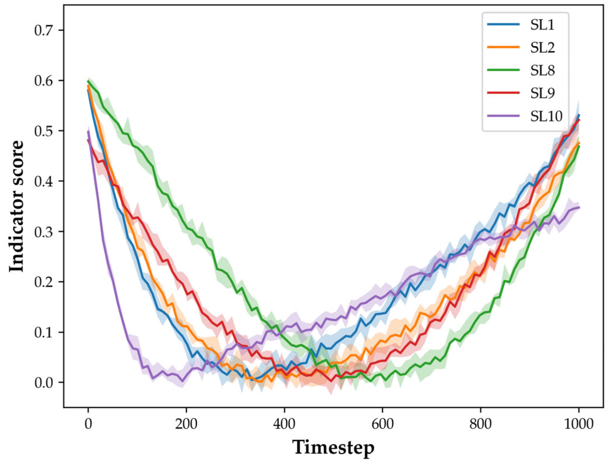
3.1.5. Timestep Adaptive Module

The timestep largely determines the quality of reconstructed images. Relevant experiments and research [27,33] show the single valley function relationship between timestep and the quality of reconstructed images. In this article, the advance–retreat method is adopted as the core concept of the timestep adaptive module. It is a dominant optimization algorithm, with adjusted search steps to achieve the closest optimal solution in accordance with the change in objective function.

The timestep adaptive module is illustrated in Figure 4.

The training data for the feature extraction of defect-free surfaces are defect-free images only. In consideration of this, SSIM and MSE served as evaluation indicators to ensure the reconstruction result is maximally similar to the original image, which can be defined as follows:

$$𝕃=(1-\alpha )MS{E}_{x,y}+\alpha (1-SSI{M}_{x,y})$$

(18)

where $x$ and $y$ represent the original and reconstructed data, respectively; and $\alpha$ refers to the weight factor to balance the relative importance of the pixels and SSIM. Herein, $\alpha =0.5$ is designated to balance the degree of distortion and SSIM of the images. SSIM can be calculated based on the data of brightness, contrast, and structure:

$$SSI{M}_{x,y}=\frac{(2{\mu }_x{\mu }_y+c_1)(2{\sigma }_{xy}+c_2)}{({\mu }_x{}^2+{\mu }_y{}^2+c_1)({\sigma }_x{}^2+{\sigma }_y{}^2+c_2)}$$

(19)

In the formula above, ${\mu }_x$ and ${\mu }_y$ represent the average values of $x$ and $y$, respectively; ${\sigma }_x$ and ${\sigma }_y$ denote the variance of $x$ and $y$, respectively; ${\sigma }_{xy}$ is the covariance of $x$ and $y$; $c_1={(k_{1}L)}^2$ and $c_2={(k_{2}L)}^2$ are constants to maintain stability; and $L$ stands for the dynamic range of pixel values, with $k_1=0.01$ and $k_2=0.03$ [19].

MSE can be calculated with the following formula:

$$MS{E}_{x,y}=\frac{1}{n}{\displaystyle \sum _{i=1}^n{(x-y)}^2}$$

(20)

After the initial point $T_0$ and the initial step $h=100$ are set, the next detection point can be written as $T_{100}=T_0+h$, based on which the $𝕃(T_0)$ and $𝕃(T_{100})$ can be calculated and compared. If $𝕃(T_0)\ge 𝕃(T_{100})$, the forward search can be continued, otherwise, the reverse search should be implemented, and the search step size is defined as $\frac{h}{2}$. To prevent the search from falling into an infinite loop, a counter is set herein to control the number of searches. It will stop the search and output $T_k$ when the number of cycles $n$ reaches 20.

3.2. Defect Detection with SN-DDPM

The SN-DDPM only containing the features of flawless products is obtained, as mentioned in Section 3.1, in which the corresponding optimal timestep is clarified. Here, the defect image is reconstructed, and the defect is located accurately. As shown in Figure 1b, the defect is segmented into main three steps, namely, image reconstruction, image difference, and FTSD, as specified below (Algorithm 1).

Algorithm 1: Defect Detection with SN-DDPM

Input: RGB image $X$ Output: Defect detection result $X_{result}$ 1:   Step 1: Obtaining the optimal timestep and reconstructing the defect image $\widehat{X}$. 2:   Step 2: Processing the images as follows: 3:   Converting the RGB image to grayscale: $X_{gray}=0.2125X_r+0.7154X_g+0.0721X_b$ 4:   Gaussian filter: $X_{gaussian}=\frac{1}{2\pi {\sigma }_x{\sigma }_y}\cdot \exp (-\frac{x^2+y^2}{2{\sigma }_x{\sigma }_y})$ 5:   Step 3: Absolute difference: 6:   $\Delta X=|X_{gaussian}-{\widehat{X}}_{gaussian}|$ 7:   Step 4: Performing FTSD: 8:   Applying the Gaussian filter to smooth the residual image 9:   Converting the smoothed image to LAB color space 10:    Calculating the average image feature vector 11:    Calculating the pixel vector value 12:    Calculating the saliency image from normalized Euclidean distance 13:  Step 5: Binarization: 14:    Calculating the threshold value: $T=\mu +\sigma$ 15:    Binarizing the saliency image: $O=\left\{\begin{array}{l}0,\mathrm{if}p\le T\\ 255,otherwise\end{array}\right.$ 16:  Step 6: Closed operation: 17:    $X_{result}=(X_{saliency}\oplus s)\ominus s$

Step 1: The defect image is reconstructed using the previously obtained reconstruction model and the optimal timestep. With the defect image serving as input, the optimal timestep controls the SN to generate a noisy image and input it into the reconstruction model to obtain the reconstructed image, which maximally keeps the features of flawless products, with the defects repaired.

Step 2: The grayscale processing and Gaussian filtering are conducted on defect images and reconstructed images, respectively, as expressed in Formulas (21) and (22), respectively:

$$X_{gray}=0.2125X_r+0.7154X_g+0.0721X_b$$

(21)

$$G(x,y)=\frac{1}{2\pi {\sigma }_x{\sigma }_y}\cdot \exp (-\frac{x^2+y^2}{2{\sigma }_x{\sigma }_y})$$

(22)

where, $X_{gray}$ represents the grayscale image; and $X_r$, $X_g$, and $X_b$ are the pixel values of the red, green, and blue (RGB) channels, respectively. Meanwhile, the convolution kernel with the size of 3 × 3 is selected for Gaussian filtering, and ${\sigma }_x$ and ${\sigma }_y$ denote the pixel deviations in the x-axis and y-axis directions of the image, respectively.

Step 3: The absolute difference operation (Formula (23) is performed on the test diagram and the reconstructed grayscale Gaussian image to obtain a residual image.

$$\Delta x_{(m,n)}=|x_{(m,n)}-{\widehat{x}}_{(m,n)}|$$

(23)

In the expression above, $x_{(m,n)}$ and ${\widehat{x}}_{(m,n)}$ represent the standard image and operated image with the dimension of $m\times n$, respectively, and $\Delta x_{(m,n)}$ refers to the residual image.

Step 4: The residual image is subjected to FTSD to obtain a saliency image. As demonstrated in Figure 5, the specific process includes smoothing the residual image using a 7 × 7 Gaussian filter to eliminate noise and preserve the overall structure of the image. The image obtained at this time is called a Gaussian image, which is then converted from the RGB color space to the LAB color space to obtain the Lab image. Subsequently, the average pixel values $L_{\mu }$, $a_{\mu }$, and $b_{\mu }$ of the L, A, and B channels of the converted Lab image are calculated to obtain the average image feature vector $I_{\mu }$ and pixel vector value $I_{\omega hc}(x,y)$. After the calculation and normalization of the Euclidean distance of these two vectors, the saliency image is finally obtained.

Step 5: The random noise in the unreal defect area is filtered for more accurate detection. Noise usually obeys a normal distribution, so binarization is employed to segment a gray residual image, with the threshold being defined as follows:

$$T=\mu +\sigma$$

(24)

where, $T$ is the adaptive threshold, and $\mu$ and $\sigma$ are the mean and standard deviation of the saliency image, respectively. The binarization and segmentation operations are expressed as follows:

$$\left\{\begin{array}{l}p=0,p\le T\\ p=255,p>T\end{array}\right.$$

(25)

where $p$ represents the pixel value of the residual image; 0 is defined if $p$ is less than or equal to the threshold, otherwise 255 is designated.

Step 6: Finally, through a closed operation, small holes are eliminated, and cracks in the contour line are filled, thus obtaining a complete defect form. The closed operation is expanded and corroded, with the formula as follows:

$$X_{result}=(X_{saliency}\oplus s)\ominus s$$

(26)

where $X_{result}$ is the image after the closed operation, $s$ represents the structural element, $\oplus$ is the expansion operation, and $\ominus$ refers to the corrosion operation.

The spatial complexity of the SN-DDPM model is significant, with 239.6 M parameters, each of which is stored using a 32-bit floating point data type. Such a large set of parameters endows SN-DDPM with powerful characterization capabilities, enabling it to extract more subtle patterns and associations, giving it an advantage in complex conditions, large-scale datasets, or high-dimensional data.

4. Experimental Setup

4.1. Datasets

The colored fabrics from the small lattice (SL) dataset from the Yarn-dyed Fabric Image Dataset Version 1 (YDFID-1) [34] were selected, which consisted of 3245 defect-free samples and 254 defect samples. The fabric pattern is primarily that of small lattices, displayed in RGB images of 512 × 512 pixels. To verify the applicability of SN-DDPM on different color fabrics, eight types of typical fabrics with different textures and colors were selected, which are SL1, SL2, SL5, SL8, SL9, SL10, SL11, and SL13. Images of some defect-free and defect samples were selected for comparison, as given in Figure 6. This dataset contains highly complicated defect categories and fabric textures, providing a sound solution for verifying the performance of deep learning models in detecting complicated defects.

Influenced by insufficient data of defect-free samples in the dataset, the sample size was increased using data enhancement methods, which is beneficial for improving the model invariance. A total of 51,888 high-quality images were obtained by rotating the original defect-free images at 90°, 180°, and 270°, as well as flipping the upper, lower, left, and right mirror surfaces. They served as training sets, while the rest of the samples were test sets.

4.2. Training Process

During the model training, the flawless fabric image was adopted only to train fully extracting the characteristics of flawless samples with the principle of unsupervised learning. The model was trained through flawless images, obtaining the feature distribution of these samples. The detection results of the proposed method were compared with those of DCAE [35], DCGAN [36], Recycle-GAN [37], MSCDAE [38], UDCAE [39], VAE-L2SSIM [40], and AFFGAN [12]. All models were trained with a batch size of 8, an epoch of 5000, and a learning rate of 1 × 10⁻⁴. Meanwhile, the model loss should be maintained in a stable state. A system equipped with an Intel i9-12900H CPU and Nvidia RTX3070ti GPU was employed to train and test the models in this article.

4.3. Evaluation Method

4.3.1. Evaluation Indicator of Image Reconstruction Results

The peak signal-to-noise ratio (PSNR) [41] and SSIM, two commonly applied indicators to assess image quality, can quantitatively analyze the reconstruction results and evaluate the model’s capability to retain details during image reconstruction objectively and accurately. SSIM was discussed in Section 3.1.5, and PSNR is introduced herein.

By combining Formula (20), the PSNR can be defined as follows:

$$PSNR=10{\log }_{10}(\frac{MA{X}_I^2}{MSE})$$

(27)

$MA{X}_I^2$ in the above expression represents the maximum possible pixel value of the image. The image pixels used in the article are represented by 8-bit binary, so its value is 255.

With large PSNR and SSIM values, the reconstruction model can better preserve the details of the original image, the reconstruction results are closer to the original image, and the image quality is higher. Therefore, the larger the values of PSNR and SSIM, the higher the similarity between the reconstructed image and the original image, and the stronger the model’s capability to reconstruct details.

4.3.2. Evaluation Indicator Defect Detection Results

Precision (P), recall (R), accuracy (Acc), F1 value, and intersection over union (IoU), as defined in Formulas (28)–(32), were employed to quantitatively analyze the defect detection results of different models.

$$P=\frac{TP}{TP+FP}\times 100\%$$

(28)

$$R=\frac{TP}{TP+FN}\times 100\%$$

(29)

$$Acc=\frac{TP+TN}{TP+FP+TN+FN}\times 100\%$$

(30)

$$F1=\frac{2\times TP}{2\times TP+FP+FN}\times 100\%$$

(31)

$$IoU=\frac{TP}{TP+FN+FP}\times 100\%$$

(32)

The relationships among the four indicators, true positive ($TP$), false positive ($FP$), false negative ($FN$), and true negative ($TN$), are summarized in Figure 7, with gray representing the test result and brown representing the reference value. Actually, $TP$ represents the number of pixels that are successfully detected and confirmed as defect areas; $FP$ represents the number of pixels that are defect areas but erroneously identified as non-defective areas; $FN$ refers to the number of pixels that are non-defect areas but erroneously identified as defective areas; and $TN$ stands for the number of pixels which are successfully detected and confirmed as defect-free areas. $P$ and $R$ denote the precision of the model in predicting whether it is correct or not. The higher the $P$ and $R$ values, the better the performance of the defect detection method. Nevertheless, it is worth noting that there are contradictions between $P$ and $R$ under certain circumstances, increasing the difficulty in acquiring higher values of both, while the $F1$ value can better reflect the overall detection performance. In addition, $Acc$ indicates the model’s accuracy in predicting the correct region, and $IoU$ measures the accuracy of the model in judging the defect position. $Acc$ and $IoU$ can reflect whether the model has detected the defect, instead of unilaterally paying attention to the accuracy of defective pixel detection.

5. Experimental Results and Discussion

5.1. Fabric Images Reconstruction Experiments

The reconstruction capability of the unsupervised detection model has a direct effect on the detection results, which is primarily reflected in the repair of the defect area of the detected fabric image and that of the image details of the defect-free area. For comparing the reconstruction capabilities of DCAE, DCGAN, Recycle-GAN, MSCDAE, UDCAE, VAE-L2SSIM, AFFGAN, and SN-DDPM, the fabric samples with different textures, background colors, and types of defects were selected in this study. Figure 8 shows the repairing results of eight models on the image to be tested, in which the sample SL1 contains a large defect area. The DCGAN and VAE-L2SSIM exhibit no remarkable defect areas but fail to visualize details of the defect-free areas. The reconstructed image of DCGAN displays obvious stitching traces, while that of VAE-L2SSIM possesses blurring and texture disorder. The DCAE, MSCDAE, AFFGAN, and UDCAE all show traces of defect areas, of which the reconstructed results of MSCDAE are quite different from the original images. Recycle-GAN cannot effectively reconstruct defect areas into good products, and there is a big difference between non-defect areas before and after reconstruction. Compared with the above six models, SN-DDPM shows higher capability to repair defect areas and displays the non-defect areas almost the same as the original images, which is beneficial to the subsequent defect positioning. The second line shows the sample SL8 with monofilament stripe defects and the construction and repair results of each model. After repair by the DCAE, DCGAN, and VAE-L2SSIM, traces of defect areas are not observed, but the texture information of non-defect areas is lost. Furthermore, block stitching traces are visible in the reconstructed images after repair by DCGAN. MSCDAE retains the defects on the reconstruction diagram, and the reconstruction results of non-defect areas are not as good as expected. Additionally, UDCAE is unable to effectively reconstruct the images and Recycle-GAN fails in and enlarges the defect area. In addition, AFFGAN is capable of effectively reconstructing a defect image into a defect-free image but exhibits a too regular and unnatural texture of the reconstructed image compared with the original image. The above comparison and discussion reveal that SN-DDPM possesses leading advantages in repairing defect areas and maintaining relevant details of non-defect areas. The results of eight models in reconstructing and removing small defects in sample SL9 containing small defects are listed in the third row. It can be observed that most models exhibit the repaired defect areas. Nevertheless, VAE-L2SSIM and DCGAN fail to effectively reconstruct the image, while Recycle-GAN and MSCDAE suffer from blurred reconstructed images and defect retention. Therefore, SN-DDPM has a better visual reconstruction effect of texture details than that of other models, thus reasonably demonstrating competitive reconstruction performance.

Furthermore, PSNR and SSIM are selected to assess the image quality, based on which the reconstruction capabilities of various models are quantitatively compared. There is no defect-free image corresponding to the defect sample in the data set so the defect-free image is used as the reconstruction object. As listed in

Table 1. PSNR and SSIM values in the reconstructed images of 7 models.

Index	Method	SL1	SL2	SL5	SL8	SL9	SL10	SL11	SL13	Average Value
SSIM	DCAE	0.9584	0.8035	0.8264	0.9341	0.6942	0.8907	0.7530	0.8886	0.8436
	DCGAN	0.5477	0.1682	0.5392	0.0986	0.7462	0.3840	0.3568	0.0460	0.3608
	Recycle-GAN	0.0151	0.2721	0.1397	0.3643	0.0787	0.3472	0.1495	0.0330	0.1750
	MSCDAE	0.4084	0.4238	0.1586	0.3286	0.7645	0.3988	0.4672	0.4385	0.4236
	UDCAE	0.9558	0.7956	0.8234	0.8267	0.8564	0.8462	0.7869	0.7093	0.8250
	VAE-L2SSIM	0.5703	0.1699	0.3295	0.3885	0.4695	0.4629	0.5428	0.3921	0.4157
	AFFGAN	0.9748	0.8542	0.8594	0.8693	0.9135	0.9491	0.9446	0.9136	0.9098
	SN-DDPM	0.9646	0.9029	0.8697	0.8938	0.9396	0.9077	0.9481	0.9591	0.9232
PSNR (dB)	DCAE	26.2641	26.7438	27.4138	27.1108	24.9037	28.3805	27.9167	28.6731	27.1758
	DCGAN	14.8116	12.8657	14.5869	8.1876	14.6379	13.8489	13.2846	12.2010	13.0530
	Recycle-GAN	11.7674	17.5644	11.7564	18.3723	18.9168	19.0082	14.6736	11.0379	15.3871
	MSCDAE	19.9604	21.7564	12.4692	14.8990	24.9513	23.1437	21.2004	25.1333	20.4392
	UDCAE	25.3496	25.6432	25.3891	22.8675	26.3204	25.6267	21.9769	25.0596	24.7791
	VAE-L2SSIM	20.8485	10.0348	12.8676	24.6738	18.7857	22.9767	20.6472	26.1235	19.6197
	AFFGAN	28.1567	28.9947	27.0947	27.8877	28.9254	29.3189	30.0192	27.7191	28.5146
	SN-DDPM	28.1464	29.8400	25.4589	27.8956	29.1771	30.2919	28.3950	30.1329	28.6672

Note: The optimal result is marked with a bold number.

, SN-DDPM obtains the best SSIM values, which verifies that the timestep adaptive module constrained by SSIM can effectively improve the reconstruction capability of the model in defect-free areas. In addition, SN-DDPM also obtains the highest PSNR values, indicating that this model has strong a reconstruction capability. Notably, both AFFGAN and SN-DDPM can capture the structural and textural features of fabrics, but the pixels of the reconstructed image using AFFGAN on the sample SL11 are closer to those of the original image. Thus, AFFGAN and SN-DDPM demonstrate close SSIM but greatly different PSNR.

The above results suggest that DCGAN learns the features of defect-free regions, so that it can effectively reconstruct the defect regions. The block reconstruction of the DCGAN model on the image results in the failed connection of the fabric textures in the adjacent grid boundary areas, causing obvious stitching marks in the reconstruction results. The partially reconstructed images by DCAE, MSCDAE, and UDCAE demonstrate observable defects. Due to fewer network layers and smaller receptive domains, DCAE and MSCDAE are applicable for simple mapping transformations on input images only, making it difficult to extract the essential texture information of flawless areas. In comparison with DCAE and MSCDAE, the UDCAE model presents poor connections among image pixels even though the network structure has been deepened. As a result, the deep model compresses the images by force, so that some details are lost. In addition, the overall color scale is similar, so that it is easy to form the color block kernels, as observed in the sample SL8, intensifying the difficulty of accurately positioning the defects. AFFGAN enhances the feature representation capability of defect-free textures based on the attention mechanism, maintaining good reconstruction results. Notably, some reconstruction results still are subjected to a small number of residual defects. As observed in the reconstructed image of SN-DDPM, the defect areas in the color-patterned fabric image are repaired, and features of the defect-free areas are clearly and intuitively displayed. This indicates that SN-DDPM exhibits the best performance in capturing the essential information of color-patterned fabric images. In addition, detail textures are concerned more with introducing a timestamp adaptive module guided by SSIM and MSE, achieving optimal reconstruction and restoration results.

5.2. Defect Detection Experiments

To verify whether the SN-DDPM can accurately locate the defects at the pixel level, relevant tests were performed on fabric samples containing different textures, background colors, and types of defects. The overall results are shown in Figure 9, where the original images, reconstructed images, heat maps, saliency images, final results, and ground truth are displayed in sequence from top to bottom. As shown in the third lines (heat maps), SN-DDPM performs well in the reconstruction of defect images, so the reconstruction error of defect-free areas exerts a small influencing effect on the detection results. In addition, the saliency images in the fourth line suggest that the salient algorithm can accurately segment defects and highlight defect areas, exhibiting obvious effects on small defects with low contrast in samples SL11 and SL13. The final results are extremely close to the ground truth except for the sample SL5. However, because of the similarity between the defect color and the background color, the sample SL5 suffers significant pixel loss in the defect area during the absolute difference process, resulting in incomplete defect morphology in the saliency image. However, this does not influence the capability to determine the shape and location of the defects based on the detection results. Therefore, applying SN-DDPM for defect image reconstruction and combining saliency algorithms for defect detection can achieve excellent results and high reliability in defect positioning.

To evaluate the performance of SN-DDPM objectively and accurately,

Table 2. Model detection accuracies on various types of fabrics.

Metric (%)	Method	SL1	SL2	SL5	SL8	SL9	SL10	SL11	SL13	Average Value
P	DCAE	37.92	37.73	48.87	63.49	16.29	46.59	55.83	47.52	44.28
	DCGAN	22.29	38.13	66.45	31.91	16.23	8.76	0.00	0.00	22.97
	Recycle-GAN	36.24	25.39	20.33	42.77	31.25	23.85	35.78	44.15	32.47
	MSCDAE	51.39	36.17	49.68	56.78	44.68	43.66	54.09	49.68	48.27
	UDCAE	54.94	55.55	87.75	15.53	59.14	51.14	15.69	87.75	53.44
	VAE-L2SSIM	0.00	42.69	25.00	70.13	14.28	24.48	2.28	24.06	25.37
	AFFGAN	62.01	17.02	21.84	63.26	35.85	47.69	34.67	29.86	39.02
	SN-DDPM	61.10	58.97	33.48	57.45	60.47	51.04	61.44	46.10	53.76
R	DCAE	72.92	65.04	51.57	81.08	13.51	62.74	60.03	65.80	59.09
	DCGAN	20.08	35.93	6.70	17.73	10.00	1.00	0.00	99.44	23.86
	Recycle-GAN	79.56	60.22	56.68	73.87	67.80	83.46	74.28	75.27	71.39
	MSCDAE	74.44	74.15	71.15	86.55	26.03	71.23	76.19	71.15	68.86
	UDCAE	82.11	61.61	35.66	8.08	78.45	44.20	15.12	35.66	45.11
	VAE-L2SSIM	0.00	14.14	0.99	59.60	22.50	2.81	11.66	34.10	18.22
	AFFGAN	75.89	57.42	69.09	79.30	80.57	64.41	38.12	44.79	63.70
	SN-DDPM	83.07	70.61	87.01	84.20	64.11	83.65	80.89	76.92	78.81
Acc	DCAE	98.36	97.85	96.97	99.23	97.99	98.59	99.26	99.37	98.45
	DCGAN	97.63	98.93	97.03	99.17	97.84	98.84	99.15	0.00	86.07
	Recycle-GAN	99.09	97.69	97.47	99.05	98.26	99.01	99.25	99.10	98.62
	MSCDAE	98.78	97.52	94.92	99.24	98.23	98.53	99.23	94.92	97.67
	UDCAE	98.94	98.74	97.84	99.00	98.67	98.75	99.21	97.84	98.62
	VAE-L2SSIM	98.68	98.72	96.90	99.36	98.27	98.85	99.53	99.53	98.73
	AFFGAN	99.16	97.34	97.97	99.23	99.82	98.66	99.17	99.55	98.86
	SN-DDPM	99.36	97.87	97.61	99.40	99.42	99.42	99.62	98.90	98.95
F1	DCAE	46.55	46.41	48.02	67.26	14.74	50.17	52.60	45.36	46.39
	DCGAN	16.32	36.24	10.48	21.72	5.36	1.75	0.00	0.00	11.48
	Recycle-GAN	46.05	24.97	27.65	0.00	37.88	33.31	44.08	52.51	33.31
	MSCDAE	58.40	47.29	57.64	66.59	25.68	51.90	59.66	57.64	53.10
	UDCAE	63.17	53.36	46.99	8.63	60.60	39.22	13.14	46.99	41.51
	VAE-L2SSIM	0.00	19.34	1.90	63.68	15.04	4.86	22.42	22.42	18.71
	AFFGAN	65.15	16.41	31.53	66.57	49.62	52.57	32.35	29.93	43.02
	SN-DDPM	65.62	55.61	44.77	64.67	61.44	57.11	64.76	54.20	58.52
IoU	DCAE	31.45	31.85	32.98	52.24	23.87	34.98	38.03	30.42	34.48
	DCGAN	10.11	28.70	6.69	15.12	2.96	0.99	0.00	0.00	8.07
	Recycle-GAN	33.22	16.81	16.54	38.22	23.83	21.54	30.60	39.17	27.49
	MSCDAE	42.80	31.25	44.59	50.91	17.45	36.50	44.07	44.59	39.02
	UDCAE	47.31	39.43	32.49	6.39	44.06	26.37	8.62	32.49	29.65
	VAE-L2SSIM	0.00	13.40	0.99	48.65	9.44	2.75	12.76	12.76	12.59
	AFFGAN	50.09	9.33	19.18	51.32	33.00	37.14	25.48	20.84	30.80
	SN-DDPM	53.25	47.25	31.52	50.94	48.92	46.80	54.09	40.26	46.63

Note: The optimal result is marked with a bold number.

presents the values of evaluation indicators of DCAE, DCGAN, Recycle GAN, MSCDAE, UDCAE, VAE-L2SSIM, AFFGAN, and SN-DDPM in each test set. In terms of average value, SN-DDPM achieves the optimal results in all indicators, of which the F1 and IoU values typically reflect an increase in model performance by at least 5.42% and 7.61%, respectively. The table reveals that UDCAE is comparable to SN-DDPM in terms of P and Acc values but exhibits a significantly lower F1 value. This is attributed to the fact that compared to SN-DDPM, UDCAE shows poorer detection results in the ground truth, which can be expressed as a larger FN in the confusion matrix diagram. Due to the higher number of pixels in the defect-free region, AFFGAN maintains a higher Acc value but a higher FP rate in recognizing the defects, resulting in lower P and F1 values. The P and R values of SN-DDPM are basically complementary, indicating that when the P value is positive, the R value is negative, and vice versa. Compared to other models, the difference between the lower and higher performance values of SN-DDPM is not significant, which is more intuitive in the F1 value. Such a result suggests that SN-DDPM improves the F1 value significantly, demonstrating its superiority in overall detection performance. Meanwhile, SN-DDPM demonstrates its advantage in Acc value, although it is not so significant in comparison to other models. The primary reason is that the number of pixels in the defect areas used is much smaller than that in the defect-free area, rendering Acc unable to objectively describe the quality of the detection results. Referring to the value of IoU, SN-DDPM is highly competitive, with the highest IoU values, demonstrating its accuracy and reliability in defect prediction.

5.3. Ablation Study

The effectiveness of the timestep adaptive module is based on the condition that the evaluation indicator $𝕃$ is a single valley function because it is difficult to solve the optimal timestep in case L is a multi-valley function. The defect-free samples SL1, SL2, SL8, SL9, and SL10 are selected as the experimental subjects to verify whether the evaluation indicator $𝕃$ is a single valley function. Specifically, $𝕃$ is calculated every 10 steps, with a total timestep of 1000. The experimental results are illustrated in Figure 10.

The figure discloses that the evaluation indicators of various samples show the characteristics of a unimodal function. Some fluctuations in the waveform activate within the error range and are free from significant influence on the overall trend. In addition, a lower value of L reflects a better reconstruction effect. Based on the optimal step sizes corresponding to various types of samples, it can be observed that all results are within the range of 0–1000 and are different in each type of sample. In this case, it is impossible to represent the optimal step sizes with fixed values, which further proves the effectiveness and applicability of the timestep adaptive module.

To further verify the validity of $\alpha =0.5$ in Formula (18), $\alpha$ is assigned different values based on the above experiments, and the optimal timestep is obtained by the timestep adaptive module. Meanwhile, the F1 and IoU values of the final result are calculated as the evaluation criteria, as listed in

Table 3. Ablation study for different values of $\alpha$.

Metric (%)	α	SL1	SL2	SL8	SL9	SL10	Average Value
F1	0.1	32.45	29.17	29.94	30.17	30.74	30.49
	0.3	58.51	55.56	56.83	47.00	52.13	54.01
	0.5	65.62	55.61	64.67	61.44	57.11	60.89
	0.7	49.00	46.05	47.95	43.26	41.46	45.54
	0.9	24.27	25.80	23.08	26.51	24.12	24.76
IoU	0.1	19.81	17.11	17.62	17.77	18.16	18.09
	0.3	41.89	38.93	40.35	30.71	35.25	37.43
	0.5	53.25	47.25	50.94	48.92	46.80	49.43
	0.7	26.10	33.22	35.01	29.95	28.19	30.49
	0.9	14.98	16.24	14.28	16.53	14.89	15.38

Note: The optimal result is marked with a bold number.

.

As observed in Table 3, the results of F1 and IoU values are not satisfactory at $\alpha =0.1$ and $\alpha =0.9$ but are the best at $\alpha =0.5$. These outcomes suggest that $\alpha =0.5$ balances the degree of distortion and structural similarity of the image. Meanwhile, the experimental results in this article confirm that $\alpha =0.5$ is effective.

5.4. Model Failure Experiment

SN-DDPM exhibits strong reconstruction performance but has insufficient robustness during the experimental process. Specifically, the reconstruction results are chaotic when there is an overwhelming number of sample types during the model training. To ensure the diversity of training samples, all fabric samples (19 types in total) in the dataset are selected as the training set, with equal numbers of each sample type, while some defect images serve as the test set. The experimental results are summarized as follows (Figure 11):

As shown in Figure 11, only the samples SL1 and SL5 can be reconstructed normally, while the reconstruction results of the remaining samples show significant pixel deviations. The texture of the defect-free area in sample SL7 is matched to that of the original image, while its color is closer to that of the sample SL2. By contrast, the samples SL2, SL3, and SL9 not only showed significant pixel deviations but also failed to reconstruct the texture details normally. Therefore, it can be concluded that SN-DDPM exhibits good detection only by training a small number of types of samples, while it has to be retrained or structurally adjusted based on different data distributions and its features adapted to other types of defect detection tasks. Consequently, it is not feasible as a unified model for all defect detection tasks.

Relevant research [42,43] shows that the major challenge faced by the diffusion model is the instability and inconsistency of the output, failing to accurately associate attributes with its objects (e.g., color). In this article, SN-DDPM demonstrates weak reconstruction results in the presence of multiple sample datasets, showing that its generalization capability still needs to be studied and improved. Therefore, the following two methods are proposed: (1) Using the mask-based SN-DDPM, the image can be reconstructed well by masking the suspicious defect areas and utilizing the defect-free features around the mask. Meanwhile, it can preserve the semantic information of the defect-free areas in the original image. Thus, the repaired image will better match the viewer’s understanding of the scene and objects, effectively avoiding the chaotic reconstruction caused by excessive training features in the model. (2) Attention mechanisms can be introduced to help the model better focus on important regions and features in the image, thereby improving the accuracy and consistency of the generated output. Through learning attention weights, the model can better comprehend the attributes and associations of objects, thereby outputting more accurate results.

6. Conclusions

In this article, a timestep-adaptive-diffusion-model-oriented unsupervised detection method is applied to the detection of fabric surface defects. It only employs the fabric defect-free samples to train the model and takes SSIM and MSE as the guided timestep adaptive modules to obtain the optimal timestep. During the detection, SN-DDPM with the optimal timestep is employed to reconstruct the defect image into a defect-free image. After that, the residual images before and after reconstruction are processed through FTSD to highlight the defect area. Finally, a discrimination threshold is utilized to segment the defect. Experimental results based on public datasets reveal that SN-DDPM can more effectively extract the essential characteristics of fabrics in contrast to other unsupervised reconstruction models. Meanwhile, its reconstruction results are closer to the true feature distribution, effectively solving the blurring, defect residue, or texture inconsistency in the reconstruction results obtained by other models. These findings suggest that the SN-DDPM demonstrates superior reconstruction capability and outstanding detection performance. In addition, the instability and inconsistency of SN-DDPM in diverse sample datasets are discussed and feasible effective solutions are recommended to help develop more reliable and powerful models.

References

1. Ngan, H.Y.; Pang, G.K.; Yung, N.H.J.I. Automated fabric defect detection—A review. Image Vis. Comput. 2011, 29, 442–458. [Google Scholar] [CrossRef]
2. Wong, W.; Jiang, J. Computer vision techniques for detecting fabric defects. In Applications of Computer Vision in Fashion and Textiles; Elsevier: Amsterdam, The Netherlands, 2018; pp. 47–60. [Google Scholar]
3. Rasheed, A.; Zafar, B.; Rasheed, A.; Ali, N.; Sajid, M.; Dar, S.H.; Habib, U.; Shehryar, T.; Mahmood, M.T. Fabric Defect Detection Using Computer Vision Techniques: A Comprehensive Review. Math. Probl. Eng. 2020, 2020, 8189403. [Google Scholar] [CrossRef]
4. Xiang, J.; Pan, R.; Gao, W. Online Detection of Fabric Defects Based on Improved CenterNet with Deformable Convolution. Sensors 2022, 22, 4718. [Google Scholar] [CrossRef] [PubMed]
5. Chen, M.; Yu, L.; Zhi, C.; Sun, R.; Zhu, S.; Gao, Z.; Ke, Z.; Zhu, M.; Zhang, Y. Improved faster R-CNN for fabric defect detection based on Gabor filter with Genetic Algorithm optimization. Comput. Ind. 2022, 134, 103551. [Google Scholar] [CrossRef]
6. Jing, J.F.; Zhuo, D.; Zhang, H.H.; Liang, Y.; Zheng, M. Fabric defect detection using the improved YOLOv3 model. J. Eng. Fiber. Fabr. 2020, 15, 1558925020908268. [Google Scholar] [CrossRef]
7. Ren, Z.; Fang, F.; Yan, N.; Wu, Y. State of the Art in Defect Detection Based on Machine Vision. Int. J. Precis. Eng. Manuf.-Green Technol. 2021, 9, 661–691. [Google Scholar] [CrossRef]
8. Szarski, M.; Chauhan, S. An unsupervised defect detection model for a dry carbon fiber textile. J. Intell. Manuf. 2022, 33, 2075–2092. [Google Scholar] [CrossRef]
9. Wang, Y.Y.; Song, K.C.; Niu, M.H.; Bao, Y.Q.; Dong, H.W.; Yan, Y.H. Unsupervised defect detection with patch-aware mutual reasoning network in image data. Automat. Constr. 2022, 142, 104472. [Google Scholar] [CrossRef]
10. Zhang, N.; Zhong, Y.; Dian, S.J.O. Rethinking unsupervised texture defect detection using PCA. Opt. Laser. Eng. 2023, 163, 107470. [Google Scholar] [CrossRef]
11. Zhang, H.W.; Chen, X.W.; Lu, S.; Yao, L.; Chen, X. A contrastive learning-based attention generative adversarial network for defect detection in colour-patterned fabric. Color. Technol. 2023, 139, 248–264. [Google Scholar] [CrossRef]
12. Zhang, H.; Qiao, G.; Lu, S.; Yao, L.; Chen, X. Attention-based Feature Fusion Generative Adversarial Network for yarn-dyed fabric defect detection. Text. Res. J. 2022, 93, 1178–1195. [Google Scholar] [CrossRef]
13. Goodfellow, I.; Pouget-Abadie, J.; Mirza, M.; Xu, B.; Warde-Farley, D.; Ozair, S.; Courville, A.; Bengio, Y. Generative adversarial networks. Commun. ACM 2020, 63, 139–144. [Google Scholar] [CrossRef]
14. Zhai, J.; Zhang, S.; Chen, J.; He, Q. Autoencoder and its various variants. In Proceedings of the 2018 IEEE International Conference on Systems, Man, and Cybernetics (SMC), Miyazaki, Japan, 7–10 October 2018; pp. 415–419. [Google Scholar]
15. Kahraman, Y.; Durmusoglu, A. Deep learning-based fabric defect detection: A review. Text. Res. J. 2023, 93, 1485–1503. [Google Scholar] [CrossRef]
16. Ho, J.; Jain, A.; Abbeel, P. Denoising diffusion probabilistic models. Adv. Neural Inf. Process. Syst. 2020, 33, 6840–6851. [Google Scholar]
17. Bansal, A.; Borgnia, E.; Chu, H.-M.; Li, J.S.; Kazemi, H.; Huang, F.; Goldblum, M.; Geiping, J.; Goldstein, T.J. Cold diffusion: Inverting arbitrary image transforms without noise. arXiv 2022, arXiv:2208.09392. [Google Scholar]
18. Perlin, K. Improving noise. In Proceedings of the 29th Annual Conference on Computer Graphics and Interactive Techniques, New York, NY, USA, 23–26 July 2002; pp. 681–682. [Google Scholar]
19. Wang, Z.; Bovik, A.C.; Sheikh, H.R.; Simoncelli, E.P. Image quality assessment: From error visibility to structural similarity. IEEE Trans. Image Process. 2004, 13, 600–612. [Google Scholar] [CrossRef]
20. Achanta, R.; Hemami, S.; Estrada, F.; Susstrunk, S. Frequency-tuned salient region detection. In Proceedings of the 2009 IEEE Conference on Computer Vision and Pattern Recognition, Miami, FL, USA, 20–25 June 2009; pp. 1597–1604. [Google Scholar]
21. Li, Y.; Zhao, W.; Pan, J. Deformable Patterned Fabric Defect Detection with Fisher Criterion-Based Deep Learning. IEEE Trans. Autom. Sci. Eng. 2017, 14, 1256–1264. [Google Scholar] [CrossRef]
22. Zhang, H.W.; Liu, S.T.; Tan, Q.L.; Lu, S.; Yao, L.; Ge, Z.Q. Colour-patterned fabric defect detection based on an unsupervised multi-scale U-shaped denoising convolutional autoencoder model. Color. Technol. 2022, 138, 522–537. [Google Scholar] [CrossRef]
23. Li, X.; Zheng, Y.; Chen, B.; Zheng, E. Dual Attention-Based Industrial Surface Defect Detection with Consistency Loss. Sensors 2022, 22, 5141. [Google Scholar] [CrossRef]
24. Zhang, H.W.; Qiao, G.H.; Liu, S.T.; Lyu, Y.T.; Yao, L.; Ge, Z.Q. Attention-based vector quantisation variational autoencoder for colour-patterned fabrics defect detection. Color. Technol. 2023, 139, 223–238. [Google Scholar] [CrossRef]
25. Wei, C.; Liang, J.; Liu, H.; Hou, Z.; Huan, Z. Multi-stage unsupervised fabric defect detection based on DCGAN. Visual Comput. 2022, 1–17. [Google Scholar] [CrossRef]
26. Zhang, G.; Cui, K.; Hung, T.-Y.; Lu, S. Defect-GAN: High-fidelity defect synthesis for automated defect inspection. In Proceedings of the IEEE/CVF Winter Conference on Applications of Computer Vision, Waikoloa, Hawaii, 3–7 January 2021; pp. 2524–2534. [Google Scholar]
27. Yang, L.; Zhang, Z.; Song, Y.; Hong, S.; Xu, R.; Zhao, Y.; Shao, Y.; Zhang, W.; Cui, B.; Yang, M.-H. Diffusion models: A comprehensive survey of methods and applications. arXiv 2022, arXiv:2209.00796. [Google Scholar]
28. Croitoru, F.A.; Hondru, V.; Ionescu, R.T.; Shah, M. Diffusion Models in Vision: A Survey. IEEE Trans. Pattern Anal. Mach. Intell. 2023, 45, 10850–10869. [Google Scholar] [CrossRef]
29. Müller-Franzes, G.; Niehues, J.M.; Khader, F.; Arasteh, S.T.; Haarburger, C.; Kuhl, C.; Wang, T.; Han, T.; Nebelung, S.; Kather, J.N.J. Diffusion Probabilistic Models beat GANs on Medical Images. arXiv 2022, arXiv:2212.07501. [Google Scholar]
30. Lugmayr, A.; Danelljan, M.; Romero, A.; Yu, F.; Timofte, R.; Van Gool, L. Repaint: Inpainting using denoising diffusion probabilistic models. In Proceedings of the IEEE/CVF Conference on Computer Vision and Pattern Recognition, New Orleans, LA, USA, 18–24 June 2022; pp. 11461–11471. [Google Scholar]
31. Li, H.; Yang, Y.; Chang, M.; Chen, S.; Feng, H.; Xu, Z.; Li, Q.; Chen, Y. SRDiff: Single image super-resolution with diffusion probabilistic models. Neurocomputing 2022, 479, 47–59. [Google Scholar] [CrossRef]
32. Gedara Chaminda Bandara, W.; Gopalakrishnan Nair, N.; Patel, V.M.J. Remote Sensing Change Detection (Segmentation) using Denoising Diffusion Probabilistic Models. arXiv 2022, arXiv:2206.11892. [Google Scholar]
33. Graham, M.S.; Pinaya, W.H.; Tudosiu, P.-D.; Nachev, P.; Ourselin, S.; Cardoso, J. Denoising diffusion models for out-of-distribution detection. In Proceedings of the IEEE/CVF Conference on Computer Vision and Pattern Recognition, Vancouver, BC, Canada, 17–24 June 2023; pp. 2947–2956. [Google Scholar]
34. Zhang, H. Yarn-Dyed Fabric Image Dataset Version 1. 2021. Available online: http://github.com/ZHW-AI/YDFID-1 (accessed on 2 August 2023).
35. Zhang, H.; Tang, W.; Zhang, L.; Li, P.; Gu, D. Defect detection of yarn-dyed shirts based on denoising convolutional self-encoder. In Proceedings of the 2019 IEEE 8th Data Driven Control and Learning Systems Conference (DDCLS), Dali, China, 24–27 May 2019; pp. 1263–1268. [Google Scholar]
36. Hu, G.; Huang, J.; Wang, Q.; Li, J.; Xu, Z.; Huang, X. Unsupervised fabric defect detection based on a deep convolutional generative adversarial network. Text. Res. J. 2019, 90, 247–270. [Google Scholar] [CrossRef]
37. Bansal, A.; Ma, S.; Ramanan, D.; Sheikh, Y. Recycle-gan: Unsupervised video retargeting. In Proceedings of the European conference on computer vision (ECCV), Munich, Germany, 8–14 September 2018; pp. 119–135. [Google Scholar]
38. Mei, S.; Yang, H.; Yin, Z. An Unsupervised-Learning-Based Approach for Automated Defect Inspection on Textured Surfaces. IEEE Trans. Instrum. Meas. 2018, 67, 1266–1277. [Google Scholar] [CrossRef]
39. Zhang, H.; Tan, Q.; Lu, S. Yarn-dyed shirt piece defect detection based on an unsupervised reconstruction model of the U-shaped denoising convolutional auto-encoder. J. Xidian Univ. 2021, 48, 123–130. [Google Scholar]
40. Wei, W.; Deng, D.; Zeng, L.; Zhang, C. Real-time implementation of fabric defect detection based on variational automatic encoder with structure similarity. J. Real-Time Image Process. 2020, 18, 807–823. [Google Scholar] [CrossRef]
41. Huynh-Thu, Q.; Ghanbari, M. Scope of validity of PSNR in image/video quality assessment. Electron. Lett. 2008, 44, 800–801. [Google Scholar] [CrossRef]
42. Du, C.; Li, Y.; Qiu, Z.; Xu, C. Stable Diffusion is Unstable. arXiv 2023, arXiv:2306.02583. [Google Scholar]
43. Chefer, H.; Alaluf, Y.; Vinker, Y.; Wolf, L.; Cohen-Or, D. Attend-and-excite: Attention-based semantic guidance for text-to-image diffusion models. arXiv 2023, arXiv:2301.13826. [Google Scholar] [CrossRef]
Figure 1. Surface defects of complicated texture fabrics: (a) linear defect; (b) spot defect; and (c) planar defect.
Processes 11 02615 g001
Figure 2. Framework of the timestep-adaptive-diffusion-model-oriented unsupervised detection method for fabric surface defects.
Processes 11 02615 g002
Figure 3. Structure of the denoising Unet.
Processes 11 02615 g003
Figure 4. Example of a timestep adaptive diagram, with the advance–retreat method applied to solve the closest solution to the optimal solution T k .
Processes 11 02615 g004
Figure 5. Process of the FTSD method to remove noise and highlight defects.
Processes 11 02615 g005
Figure 6. Images for defect-free and defect samples of colored fabrics from the SL dataset.
Processes 11 02615 g006
Figure 7. Confusion matrix diagram to show the relationship among TP, FP, TN, and FN.
Processes 11 02615 g007
Figure 8. Qualitative comparison of the reconstruction results of different models, with the red boxes marking the defect areas.
Processes 11 02615 g008
Figure 9. The defect detection effect of SN-DDPM.
Processes 11 02615 g009
Figure 10. Relationship between timestep and evaluation score for SL1, SL2, SL8, SL9, and SL10.
Processes 11 02615 g010
Figure 11. Model failure experiment: 19 types of defect-free fabric samples are trained and partial defect images are tested.
Processes 11 02615 g011