Design and Analysis of a Novel Air Bubble Curtain for Mixing and Aeration in Process Vessels

Abstract

This article focuses on designing and analyzing a new method for mixing in process vessels. We propose using an air bubble curtain to accomplish the desired mixing. The air bubble curtain used in this study is made of an empty pipe with several holes through which air is pumped, which in turn produces a swarm of bubbles that causes pseudo-turbulent mixing in the tank filled with a liquid solution. A uniform distribution of bubbles within the tank was assured by maintaining a see-saw movement of the air bubble curtain. Mixing inside the tank was quantified by measuring the salt concentration in a laboratory model tank (30 cm × 30 cm × 30 cm) and a pilot-scale tank (200 cm × 100 cm × 100 cm). The optimal flow rates of air and the mixing time in both tanks that can achieve complete mixing were obtained from the experimental results. The proposed air bubble curtain can be of potential use in wastewater treatment, biotechnology, and aquaculture where turbulent mixing is required with minimum energy dissipation per unit mass.

1. Introduction

For many years, air was used for agitating and mixing in the process industry; the recycling of newspaper; the processing of beer, dyes, and mineral pulp; oxidation; hydrogenation; biological fermentation; antibiotic development; and many other processes [1,2,3]. In aerated mixing vessels, gases and liquids come in contact with each other and are mixed to reach steady conditions and uniformity [4,5].

The choice of an effective aeration system is one of the most crucial factors in reducing energy consumption in any chemical bioengineering process. The device that usually comes to mind in connection with mixing is the conventional vessel and rotating impeller combination. Many studies have been carried out using such devices, but when attempts are made to apply the results of mixing studies, there are difficulties in obtaining the desired product [6]. The reason for this is that the results are presented in a very complicated manner with empirical correlations that are sometimes difficult to understand. Thus, for many years, chemical and civil engineers have been attracted to new mixing techniques that require less energy and have fewer operating problems. Such a technique involves mixing and agitation using air alone in many cases [7].

Furthermore, air has been used to fluidize particles in liquid and gas phases; for instance, Buckhurst et al. have determined the optimum aeration rates for the suspension of larval feeds [8]. Chaalal presented a new method that can be used to investigate the suspension of solid particles in rectangular tanks agitated by source-line bubble plumes. Chaala demonstrated the existence of a clearly defined optimum rate of aeration for a particular size of tank in batch and continuous systems. The investigation showed that the flowrate when all the particles are in suspension can be predicted, and, operating beyond that flowrate, over-aeration will occur [9].

It is known that the uniformity of any particular medium has various important applications in the field of engineering. The most desirable characteristics of aeration tanks are the uniformity and efficiency of mixing. In wastewater treatment, the mixing process makes it easier to trap harmful substances by increasing the contact area between a flocculant and an undesirable substance and helping to oxidize the activated sludge in order to provide it with favorable conditions for its metabolic activity. Additionally, uniform turbulence is conducive to the homogeneity of the treatment, and efficient aeration is requisite to the economy of operation [10]. Furthermore, the aeration process efficiency depends on several factors, such as the air mass flow rate, the depth of diffuser submergence, and the nature of the contents of wastewater. For instance, the phenomenon relating to the dispersion of a contaminant or a nutrient due to turbulent agitation is of fundamental importance when the motion is not created by a mechanical device. Jiawei Liu investigated the aeration performance of an inverted umbrella aerator and bubble characteristics in an aeration tank under different conditions; for this, an experimental bench that can measure the dissolved oxygen concentration and is also capable of high-speed photography was built. Logarithmic oxygen deficit values were fitted under various conditions [11]. Further, in 2020, Młynarczykowska published a general review on the current development of mechanically agitated vessels and presented the current state of the art in this field [12]. The review showed that advanced computational fluid dynamic techniques used for the multiphase flow analysis of reactions with modern experimental techniques can be used to successfully analyze, in detail, the mixing features in liquid–liquid, gas–liquid, solid–liquid, and multi-phase flows.

The dynamics of the fluid when air is passed through it by means of a perforated pipe have attracted many investigators, such as Bulson. Bulson pointed out that the surface current produced by the air bubble motion is the main mechanism of wave dissipation in the PB system, and empirical formulas for the surface current velocity and its thickness, as well as the required air discharge, were presented [13]. He studied the ability of currents produced by an air curtain in deep water to stop the waves in the sea. He investigated the speed of the current and the thickness of the horizontal currents produced by an air curtain in water with a depth of up to 10.4 m. Backhurst et al. investigated the possibility of using a square-shaped bioreactor agitated by an air curtain as a solution for the shear stress sensor cell. This application showed that the agitation by air alone could be a solution to the inadequate or unsatisfactory performance of mechanical agitators [4]. A recent study by Mirek showed the results of simulation calculations and practical equations for a distributor pressure drop calculation that takes into account different degrees of tuyere destruction [14]. Sir Geoffrey Taylor provided the conditions under which an outward-flowing surface current can prevent the passage of waves coming in from the sea through mathematical investigations. In the investigation, two types of current were considered: a current with a uniform velocity extending to a depth (h) and a current with a velocity decreasing uniformly and vanishing at depth (h). The water current produced by a curtain of air bubbles from a perforated tube on the sea bottom was investigated theoretically on the assumption that the bubbles are very small [15].

To illustrate, oceanographers would like to be able to determine beforehand the dispersion of waste discharged into the sea and the time for mixing which depends on the ability to uniformly disperse the material to avoid pollution. It has long been recognized that insufficient mixing in the anaerobic unit limits treatment efficiency. Uniform turbulence is conducive to homogeneity in water treatment, and efficient aeration is requisite to the economy of operation. Frankiewicz applied the steady mixing of gas–liquid systems where a significant high interfacial area is required. The study analyzes the influence of the impeller construction on the gas hold-up and volumetric mass transfer coefficient k_La. Impellers with a different number of concave blades, and with alternatively arranged concave blades, were analyzed and the obtained results were compared with the standard flat-blade turbine [16]. Cudak recorded the measurements of the mean heat transfer coefficient for the whole heat transfer surface area of the baffled jacketed agitated vessel using the steady state thermal method in a vessel of inner diameter D = 0.45 m, filled by Newtonian liquid up to the height H = D (0.5D < H < 1.9H). The measurements of the mean heat transfer coefficient for an un-baffled agitated vessel equipped with vertical tubular coils were taken using the steady-state method with a vessel with an inner diameter D = 0.6 m, filled by Newtonian or non-Newtonian liquid up to the height H = D [17].

The distribution can be described by diffusion, which generally says nothing about the distribution mechanism. The term molecular diffusion is more significant for the diffusion caused by relative molecular motion. Mixing in aerated tanks can be described by the bulk motion of large molecules called eddies, which gives rise to material transport known as eddy diffusion or dispersion.

The vast area of mixing makes it impossible to cover all aspects of mixing in an aerated tank in a single research paper. Therefore, the investigation in this paper has been limited to mixing based on the provision of air through a perforated pipe that creates an air bubble curtain as a means of mixing.

2. Experimental Apparatus and Procedure

Experiments were performed in a small laboratory tank model and in a pilot-scale model whose dimensions are shown in

Table 1. Dimensions of the tanks.

Tanks	Length (cm)	Width (cm)	Volume (L)
Model Tank	30	30	18.9
Pilot-Scale Tank	200	100	1600

.

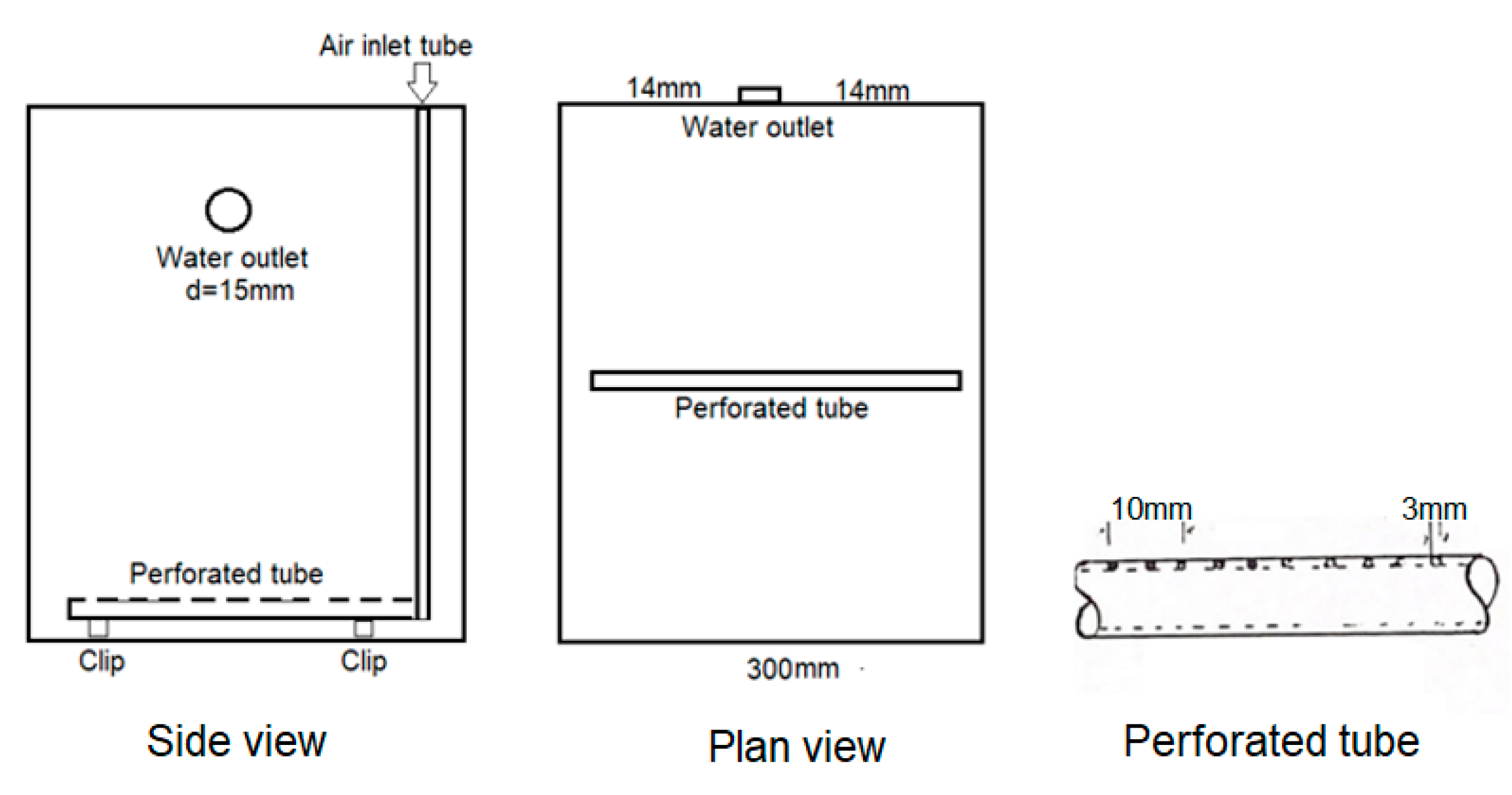
A salt solution of 1 g/L at room temperature at 18 °C was centrally prepared in the model fitted with a plastic tube (with a 6 mm internal diameter) at 1 cm from the bottom. This tube was held on the base of the tank by clips supported by plastic suction pads so that the lines of the holes were level with each other. Distilled water contained in another tank (50 cm × 30 cm × 30 cm) at the same temperature as the solution was conveyed via a rotameter to the tank by means of a centrifugal water pump, as shown in Figure 1. The air supply at 18 °C, 1.2 bar in the mixing tank, was regulated using a rotameter, and the level of water was kept constant using an overflow device (a Perspex tube with a diameter of 1 cm and a length of 3 cm sealed at the center of the tank wall 21 cm from the bottom of the tank, as shown in Figure 2). The overflowing water was tested with a conductivity meter, which showed variations in the salt concentration within the tank. The conductivity response of the solution within the tank at different time intervals and the conversion of conductivity to concentration using calibration allowed us to gather a set of exit age distribution (E) values that can be plotted against the dimensionless time (k) (which is the ratio of time to residence time, t/r) at a constant air flow rate. The shape of the graph explains the quality of the mixing that takes place in the aerated vessel. The equation of the well-mixed tank is taken as a model in order to compare the states of mixing at various air flow rates and the influence of the inlet distilled water on the concentration profile in the tank.

Equation (1) describes the variation in the salt concentration within the tank when the tank is considered well mixed.

Cm = Co e ^(−t/r)

(1)

where

Cm is the concentration in the tank or the exit concentration (g/L);

Co is the initial concentration (g/L);

t is the time (minutes);

r is the residence time (minutes).

This equation is taken as a model in order to compare the state of mixing at various air flowrates and inlet distilled water flowrates.

The air supply (at room temperature and 1.2 bar) to mixing tank 2 was regulated using a rotameter, and the level of the water was kept constant with an overflow device (a Perspex tube with a diameter of 1 cm and a length of 3 cm sealed at the center of the tank wall at 21 cm from the bottom of the tank), as shown in Figure 2.

It is well known that the best way to mix in a continuous system similar to our study is to follow the salt concentration. This method is usually used to determine how ideal mixing is achieved.

The converted conductivities to concentrations correspond to a set of exit age values at a constant air flowrate that are plotted against the dimensionless time (k) at a constant air flowrate. The shape of the graph explains the quality of the mixing that takes place in the aerated vessel.

The series of tests carried out in the model tanks to study the mixing and means of distribution of sodium chloride in the tank have shown that the exit concentration of salt is dramatically affected by the air flowrate through the pipe and the incoming distilled water flowrate.

3. Effect of Air Flowrate and Water Flowrates on Mixing

In this experiment, the water flow rate was kept equal to 0.25 L/min, and the air flow rate through the plastic tube varied from 0 L/min to 20 L/min. The overflow located at 210 mm from the base of the tank was tested, and the conductivity was recorded at intervals of 5 min for a one-hour period using a probe attached to the conductivity meter, as shown in Figure 1.

4. Results

Figure 3 displays the results of the experiment when the flow rate in the tank varied from 0 L/min to 20 L/min. It can be seen from Figure 3b that an increase in the air flowrate to 20 L/min allowed the exit concentration profile to be close to the solid line representing the perfectly mixed tank. These results provide evidence that the air flowrate is a major parameter influencing the mixing in the tank. It was observed that the bubbles form an air curtain that divides the tank into two distinct compartments. The outlet overflow was located in compartment 1 and the inlet distilled water was located in compartment 2. At an air flow rate of 10 L/min, the exit concentration was higher than the model. This can be explained by the fact that the salt concentration in compartment 1 was high compared to the salt concentration in compartment 2, into which the fresh water flows. After the solution was diluted in compartment 2, the air curtain acted as a barrier to the salt by not allowing the concentrated salt to pass to compartment 1. The exit concentration can therefore be expected to be higher in the well-mixed tank. From this experiment, it can be concluded that the tank under investigation approached the perfectly mixed vessel when the flow was about 20 L/min.

When investigating the effect, the water flow rates on mixing were maintained at 10 L/min, and the distilled water flowrate was set at 0.25 L/min for the first run and 0.50 L/min for the second run. The time for each run was about 120 min, and conductivity readings were taken at intervals of 5 min.

It is clear from Figure 3a that when the water flowrate increased, the concentration of salt in the tank decreased, and this can be noticed by the rapid decay of the exit concentration and its location far below the curve illustrating the concentration when the water flowrate was 0.025 L/min. The conclusion reached after this experiment is that the shape of the curves is constant and of exponential form, similar to that describing the perfectly mixed aerated tank. It should be noticed that the concentration plotted in Figure 3a,b is consistent with the salt age distribution E cited in the literature [18,19,20].

5. Mixing in a Pilot-Scale Tank with Stagnant Water

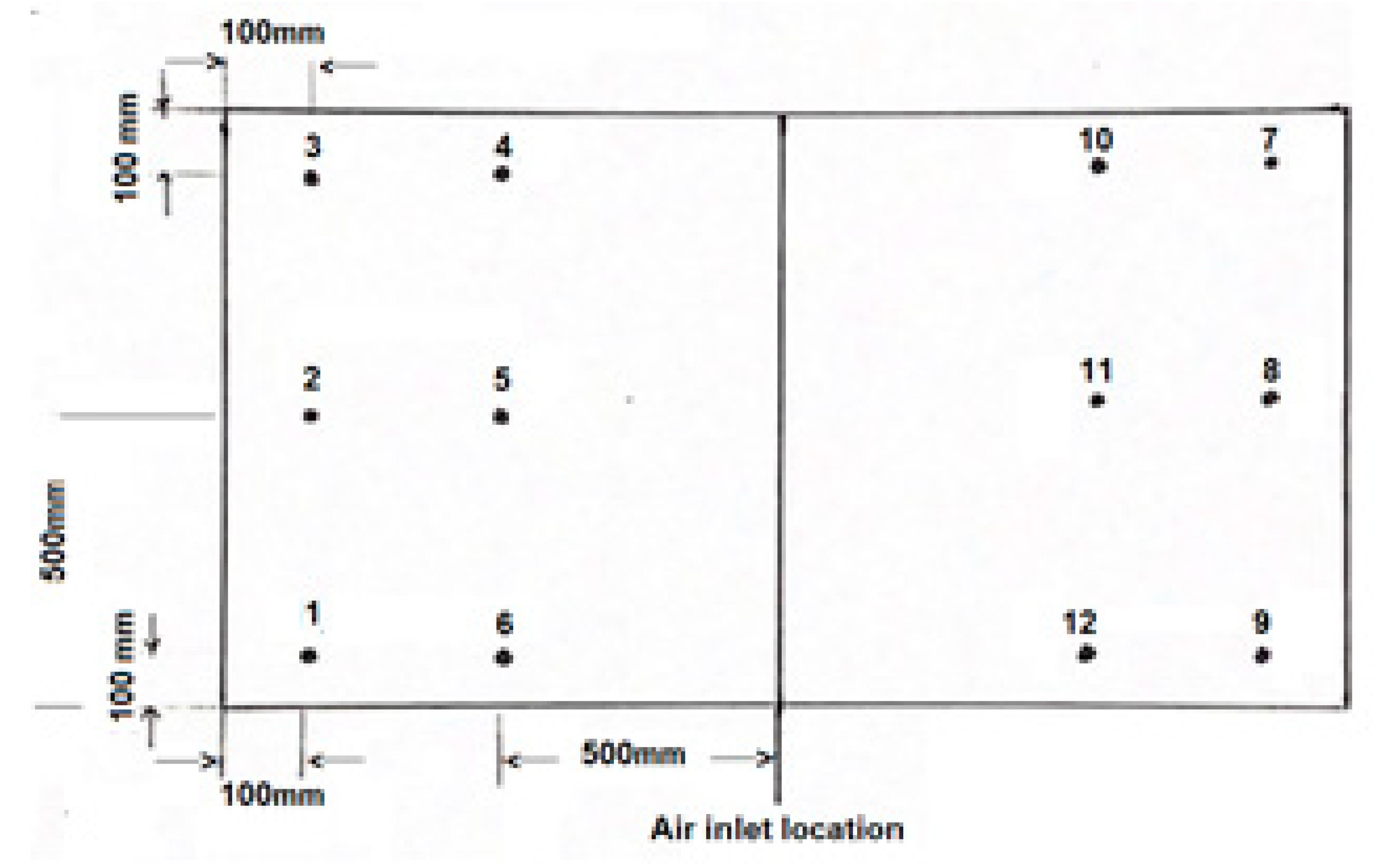
Experiments investigating the transport of salt were conducted in tanks with both stationary and agitated fresh water. The pilot tank held 1600 L of fresh water at 18 °C. A salt solution with a uniform concentration of 1 g/L was prepared in a second tank with a capacity of 200 L. This solution was discharged using a pipe (with an internal diameter of 15 mm) at a flow rate of 1 L/min set by a rotameter. The discharge point was located 5 cm from the surface of the fresh water at position 1, as shown in Figure 4.

The exit concentration of salt was determined by measuring the conductivity of the solution as follows.

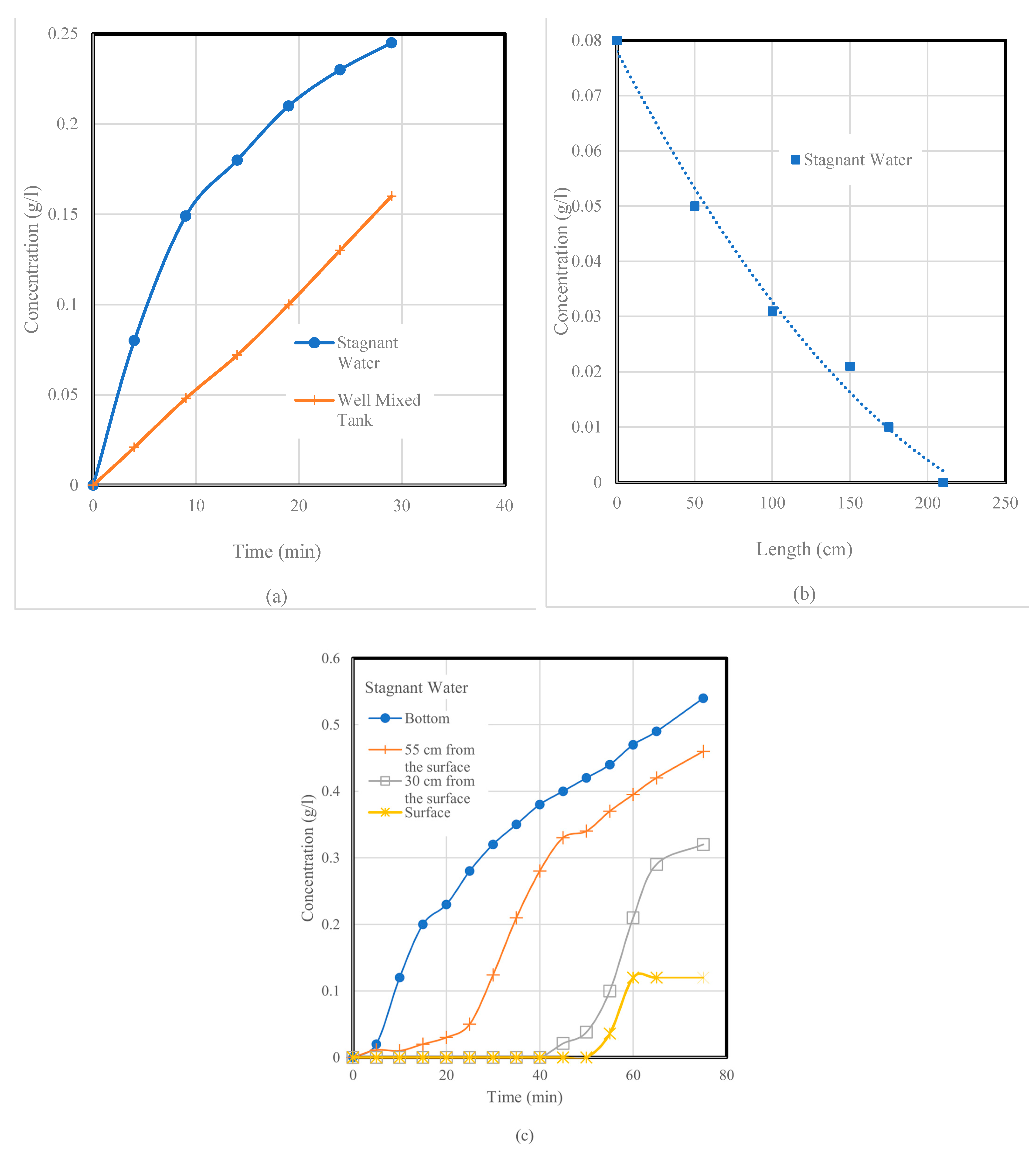
While the salt solution flowed into the tank at 1 L/min at one end of the pilot tank at position 1, the salt concentration was measured at the other end at position 9 5 cm from the bottom of the tank at intervals of 5 min using a syphon tube (with an internal diameter of 8 mm) connected to the conductivity meter. The volume of the water in the tank was assumed to be constant, and the height of the water was maintained at 800 mm. The pump operated at 1 L/min for 30 min, and the amount of salt transported to the pilot tank during the operation was 30 g. The concentration of the salt in the pilot tank, evaluated using Equation (1), was found to be equal to 0.018 g/L. Assuming that the tank was well mixed, Cm is shown as a straight line when plotted against time. The experimental curve did not follow the assumed straight line, and this could be expected since the water in the pilot tank was stagnant. The results are presented in Figure 5. The profile shown in Figure 5a represents the departure from mixing, and mixing occurred due to molar diffusion since the water was stagnant.

The curve in Figure 5b shows the concentration distribution along the length. It can be seen that at the far end of the tank, 200 cm from the salt source, the concentration was zero. In the middle of the tank, at 100 cm from the salt source, the concentration was about 0.03 g/L. The experiment data follow the exponential decay model represented by the solid line.

The results presented in Figure 5c display the concentration vs. time. At the surface, a concentration of 0.025 g/L was recorded after 55 min, and, at this time, the concentration recorded at the bottom was about 0.4 g/L. From this figure, the following observations can be made:

• All the salt was at the bottom of the pilot tank;
• The curves were similar to those quoted in the literature;
• The salt concentration was very low between the surface and 30 cm below the surface, and it took 40 min before a concentration reading could be taken.

6. Experiments on Mixing in the Pilot-Scale Tank When the Water Was Agitated

The fundamental requirement for mixing is the movement or flow of material. The case of mixing in this part falls into mixing where a salt solution is to be mixed with fresh water. The mixing here requires forced convection, whereby the bulk liquids are compelled to move by forces caused by the air curtain.

The experiments were carried out in two sets. In the first set, the salt solution was added at position 2 at a rate of 1 L/min and a depth of 800 mm. Samples were withdrawn at 5 cm from the bottom at positions (1, 3, 7, and 9 as shown in Figure 4). The samples were mixed together, and the average of the four positions was measured at intervals of 5 min. For the sample at position 1, the concentration was recorded in the same way and compared to the average concentration of the corners. The air flow rate was set at 30 L/min, and the duration of the experiment was 70 min. The results are displayed in Figure 6.

In the second set of experiments, the salt solution was added at the center of the tank, 10 cm above the air curtain, at a rate of 1 L/min. The volume of the tank and the depth of the water were shown in the experiments in the first set. Samples were taken 5 cm from the bottom seat positions (1, 3, 7, and 9) in the same way as the previous experiment, and the air flow rates used were 10 L/min, 15 L/min, 20 L/min, and 30 L/min. This experiment was conducted for 70 min. The results are displayed in Figure 7.

Figure 6 shows a net difference in concentration when the water was stagnant and when it was agitated. The concentration at one corner was the highest due to the distance from which the samples were withdrawn. When the samples from the four corners were mixed, the average concentration was lower than the one found for one corner. This can be explained by the low concentrations of the two corners situated 200 cm from the source of salt. The air blown at 30 L/min moved the water and promoted mixing. In Figure 8, the concentration is represented by a straight line, and there is no difference between the concentration at one corner and when the four samples taken from the other corners were mixed. This explains the spreading of salt throughout the tank and the good mixing that occurred in the tank.

In the results shown in Figure 7, all the experiment points are located along a straight line. Thus, the placement of the salt source near the air curtain shows that the mixing was much better at a low air flow rate of about 15 L/min, which could allow the distribution of salt to be achieved throughout the tank.

Mixing Time in the Pilot-Scale Tank

The mixing time in the pilot-scale tank was measured by means of dissolution rates of granulated sodium chloride. The mixing time was related to the air flow rate causing the aeration and mixing in the tank. In these experiments, the conductivity probe was connected to an HP computer, where the data for the conductivity were recorded in a file. These data can be printed or given as a graph. A computer program was developed to produce graphs showing the conductivity of water against time that could be seen on the computer’s screen. One kilogram of granulated salt (1 mm in size) manufactured by ICI was carefully introduced into the tank by means of a small plastic box (10 cm by 10 cm by 10 cm) and a glass tube placed at position 5. The contents of the plastic box were poured into the tube and placed vertically at position 5. This tube, with a length of 900 mm and a diameter of 60 mm, was removed from the tank when the salt reached the bottom of the tank. Samples were taken from the four corners at 5 cm from the bottom of the tank. These samples were mixed and passed through the electrode in order to measure the average conductivity.

The mixing time was recorded for completely dissolving the added salt so that it is distributed throughout the tank.. The flow rate varied from 0 L/min to 30 L/min. When the graph showed a constant value, the conductivity before all the variation in conductivity was taken as the time for complete mixing. This procedure was satisfactory and reproducible, and the results are shown in Figure 8. Figure 8 shows that the curve started to be constant after 10 min in Figure 8c when the air flow rate was 30 L/min. The graph showing the flow rate of 10 L/min (Figure 8a) showed no flattening after 30 min. Figure 8a–c shows that the optimal mixing time was 10 min. After 10 min, the concentration profile showed no change in the degree of mixing, and further continuing the experiment would lead to an increase in energy consumption.

7. Conclusions

No attempts have been made to comprehensively cover all aspects of mixing in aerated vessels using an air bubble air curtain since most tanks use mechanical agitators to promote mixing. The investigation using salt distribution in the tank gave satisfactory results and confirmed that the agitation created by air curtains leads to good mixing. Near the air bubble curtain, turbulence promoted perfect mixing, even at low air flow rates. The optimal mixing time was found to be 10 min. Applying an air bubble curtain could solve the problems encountered when mechanical agitators are known to be inadequate or unsatisfactory.