Abstract
In order to precisely ascertain the temperature at the hot spot within the intermediate joint of a three-core cable, this study focused on a 10 kV three-core cable joint as its primary subject. A three-dimensional finite element model of the cable joint was constructed, enabling the calculation of both the steady-state hot spot temperature field distribution and the transient temperature rise curve of the joint. Employing a one-dimensional transient thermal path model for the cable body, a radial inversion model for the cable core temperature was established. Through simulating the transient temperature field of the cable joint under varying currents, a fitting relationship was determined for the axial temperature points of the cable core. Subsequently, an inversion perception model was devised to calculate the hot spot temperature of the cable joint based on temperature measurements at specific points on the outer surface of the cable. Under both continuous and periodic loads, the inversion results revealed a consistent trend in the temperature at the joint crimping point with the finite element calculation outcomes, demonstrating a maximum error of within 3 degrees Celsius. This verification underscores the precision of the temperature combination inversion method when applied to three-core cable joints.
1. Introduction
As a crucial element within urban distribution networks, the functionality and well-being of three-core cables has direct significance for the secure and stable operation of the distribution network. Temperature stands out as a pivotal factor influencing the insulation performance and longevity of cable joints. In practical operations, the conductor frequently represents the highest temperature point within the insulation material. It is imperative that the temperature of the cable core does not surpass the long-term withstanding temperature of the insulation material by 90 degrees Celsius to guarantee the cable’s service life [1,2].
Owing to intricate installation procedures, substantial material dispersion, the existence of contact resistance, and the presence of diverse composite interface structures, cable joints emerge as the most vulnerable aspect in the insulation of cable systems. The conduction temperature within cable joints frequently exceeds that of the cable body, establishing a bottleneck in the cable’s thermal aging process. Consequently, undertaking temperature inversion studies on three-core cable joints holds paramount engineering significance and practical value, ensuring the secure and stable operation of power cable systems [3,4,5,6].
Various techniques are employed for monitoring the temperature of cable joints, encompassing direct temperature measurement, thermal path modeling, numerical calculation, and data mining. Ref. [7] introduced a temperature estimation method rooted in the modified thermal dynamic equilibrium approach. This method involved comparing and simulating the impacts of radiation heat dissipation, absorption heat generation, and convective heat dissipation on the temperature trend of conductors. Another approach outlined in Ref. [8] proposed the utilization of temperature-measuring optical fibers within the cable, integrated into the conductor and connected externally to the conductor connecting tube of the connecting box. These optical fibers extend to the ends of the cable line, facilitating the extraction of pre-installed optical fibers within the cable for connection to a distributed fiber optic temperature measurement system, thus enabling joint conductor temperature measurement. In a different method detailed in Ref. [9], an equivalent thermal resistance network model was employed to calculate the steady-state temperature of oil-paper insulated cable joints. This model considered dielectric loss heating and obtained the axial temperature distribution of the core in water-cooled cable joints. The study assumed axial heat flow through metal, with only radial heat flow occurring within the insulation layer.
Further investigations included Ref. [10], which utilized the two-dimensional finite element method to analyze both the steady-state and transient temperature distribution of cable joints while accounting for the variation of dielectric loss with temperature. Refs. [11,12,13] established a two-dimensional steady-state temperature analysis model based on the finite element method for cable joints. However, this model overlooked the axial heat transfer in cable joints, presenting a significant deviation from the actual scenario. Refs. [14,15] developed a back propagation neural network model for calculating the transient temperature of the intermediate joint wire core. This model incorporated measured surface temperature data from cold shrink preforms and corresponding wire core currents as inputs, yielding the transient temperature of the wire core as output. Ref. [16] employed a generalized regression neural network to predict cable joint temperatures, utilizing variables such as the left cable sheath temperature, right cable sheath temperature, left cable skin temperature, right cable skin temperature, ambient temperature, and cable current as input. The joint conductor temperature served as the output variable. With 756 sets of data used for training and 25 sets for testing, the predictive performance was satisfactory. Lastly, Ref. [17] established a simplified thermal path model for cable joints. Through formula derivation and experimentation, it was determined that the temperature rise of the metal sheath was directly proportional to the temperature rise of the cable core. The proportional coefficient, obtained experimentally, facilitated the inversion of the cable core temperature by monitoring the temperature rise of the metal sheath.
Hence, this study focused on the intermediate joint of 10 kV three-core cables, creating a research framework that established a radial inversion model of the cable core temperature. This model was rooted in a one-dimensional transient and steady-state thermal circuit model applied to the cable body. By simulating the transient temperature field of cable joints under varying currents, a fitting formula for the axial temperature point of the cable core was derived. Additionally, a reverse perception model was formulated to calculate the hot spot temperature of cable joints through temperature measurement points on the outer surface of the cable. Subsequent investigations delved into the precision of the cable joint hot spot temperature inversion method, considering the impact of material parameter dispersion.
2. Numerical Computation of Temperature Distribution in a Three-Core Cable Joint
2.1. Establishment of Simulation Model
The structural diagram of the three-core cable joint is shown in Figure 1. The joint mainly includes a cable core, pressure connection pipe, cold shrink prefabricated insulation parts, copper mesh, and external wrapping tape. After installing the three-phase joint with copper mesh, the joint was uniformly wrapped with waterproof tape outside the three joints. The main steps in its production process were: a. peeling off the outer protective layer, armor, and inner sheath; b. peeling off the copper shielding layer and outer semiconducting layer; c. peeling off the insulation layer and covering the insulation body of the joint; d. Crimping the connecting pipe and assembling the insulation body of the joint; e. wrapping it in copper mesh; and f. applying an external sealing treatment. According to Refs. [18,19,20], the specific material parameters of the 10 kV three-core cable joints are detailed in Table 1.
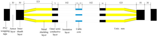
Figure 1.
Structure of 10 kV cable joint.

Table 1.
Material parameters of three-core cable joint.
During the modeling phase, several simplifications were incorporated to streamline the analysis [3,21]. Firstly, the geometric and thermodynamic parameters of each layer of the cable were treated as constant, disregarding any temperature-induced variations in these parameters. Secondly, the inner and outer shielding layers, being relatively thin, were assimilated into the insulation layer, given their similar heat capacity and thermal resistance parameters. Thirdly, considering the significantly higher thermal conductivity of the cable core compared to other insulation materials, the cable core was treated as an isothermal body with uniform heating. The conductor segment of the cable, consisting of multi-core twisted wires, was equated to a single-core circular conductor with an equivalent cross-sectional area.
Moreover, acknowledging the thinness of the copper shielding mesh and its envelopment by armor tape with substantial gripping force, its impact was neglected in the model, and a distinct copper shielding layer was not incorporated. Lastly, the influence of grounding wires was deemed negligible and thus omitted from the model.
2.2. Temperature Field Control Equation
Three categories of boundaries are pertinent to heat transfer. The initial type involves a known boundary temperature function, expressible through the following equation [22]:
In the formula, Γ represents the outer boundary of the cable; TW is the known temperature boundary, measured in K.
The second boundary condition pertains to a specified normal heat flux density at the boundary and can be expressed as follows:
In the formula, λ is thermal conductivity, n is the component in the normal direction, and q is the known heat flux density, expressed in W/m2.
The third category of the boundary condition is associated with the convective heat transfer coefficient and fluid temperature, both of which are known. It can be expressed as follows:
In the formula, α is the convective heat transfer coefficient, in W/(m2∙K); Tf is the external fluid temperature, measured in K.
2.3. Loading Conditions
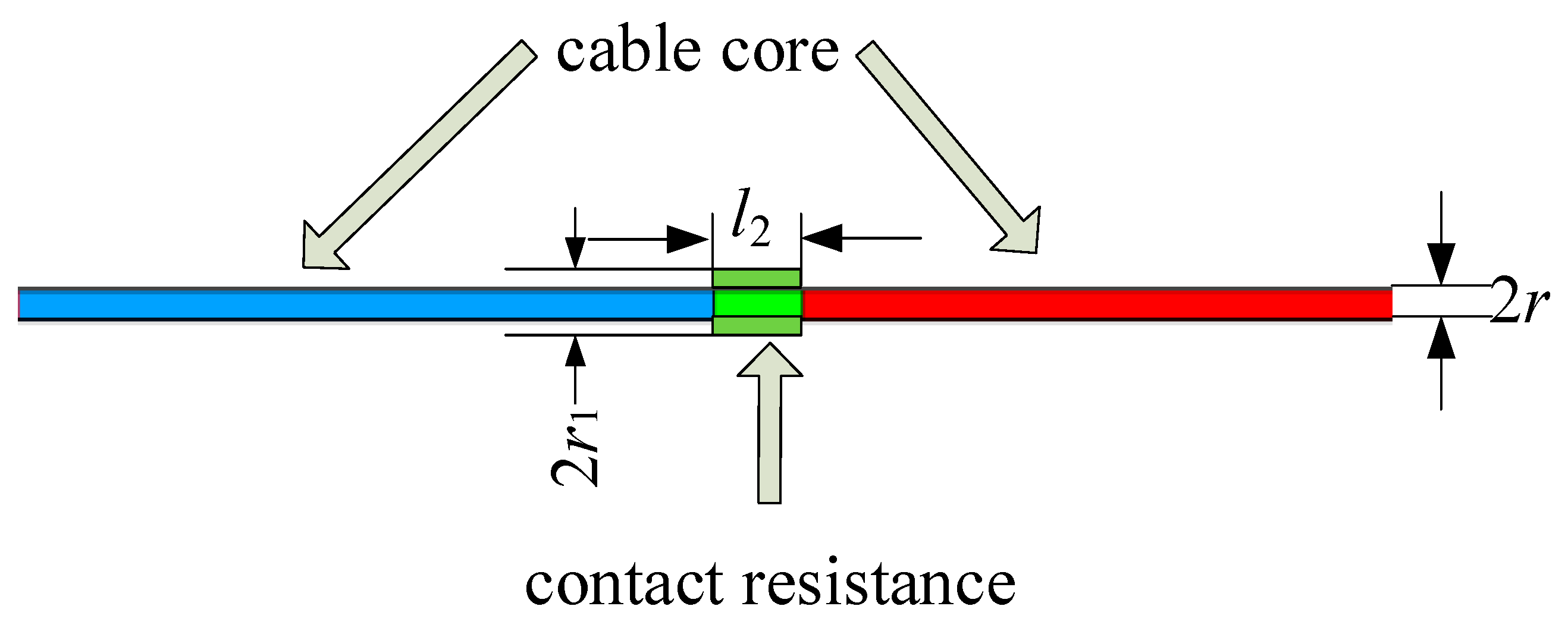
The heat source within the three-core cable joint comprises two components: heating caused by equivalent contact resistance during cable core heating and joint crimping. This can be effectively modeled by applying an equivalent heat source to a confined area near the contact surface of the joint’s long and short end conductors, as illustrated in Figure 2.
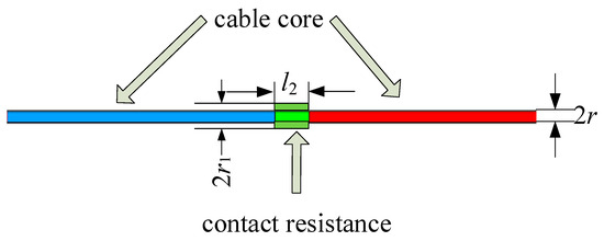
Figure 2.
Illustration of cable heat source application.
In the formula, G1 is the thermal generation rate of conductors; G2 is thermal generation rate of contact resistance; S1 is the unit cross-sectional area of the cable core; S2 is the unit cross-sectional area of the pressure connecting pipe; V1 is the unit volume of the cable core; V2 is the unit volume of the pressure connecting pipe; ρ is the resistivity of the copper conductor; l1 is the total length of the cable core; l2 is the length of the pressure connecting pipe; r is the radius of the cable core; r1 is the radius of the pressure connecting pipe; and R2 is the contact resistance of the joint and it can be calculated that G1 = I2 × 0.171 W/m3, G2 = I2 × 0.0788 W/m3.
2.4. Analysis of the Temperature Distribution in Cable Joints
The convective heat transfer boundary, representing the third temperature boundary condition, is applied to the external surface of the three-core cable joint. Utilizing an air convective heat transfer coefficient of 8 W/(m2K) [23] and an ambient air temperature of 25 °C, this boundary condition is established. The second type of temperature boundary condition is imposed at the end of the body, characterized by a zero normal heat flux density and a cable core current of 500 A. For the transient simulation, a duration of 20 h is set, and the steady-state temperature field distribution and transient temperature rise of the cable joint are calculated separately.
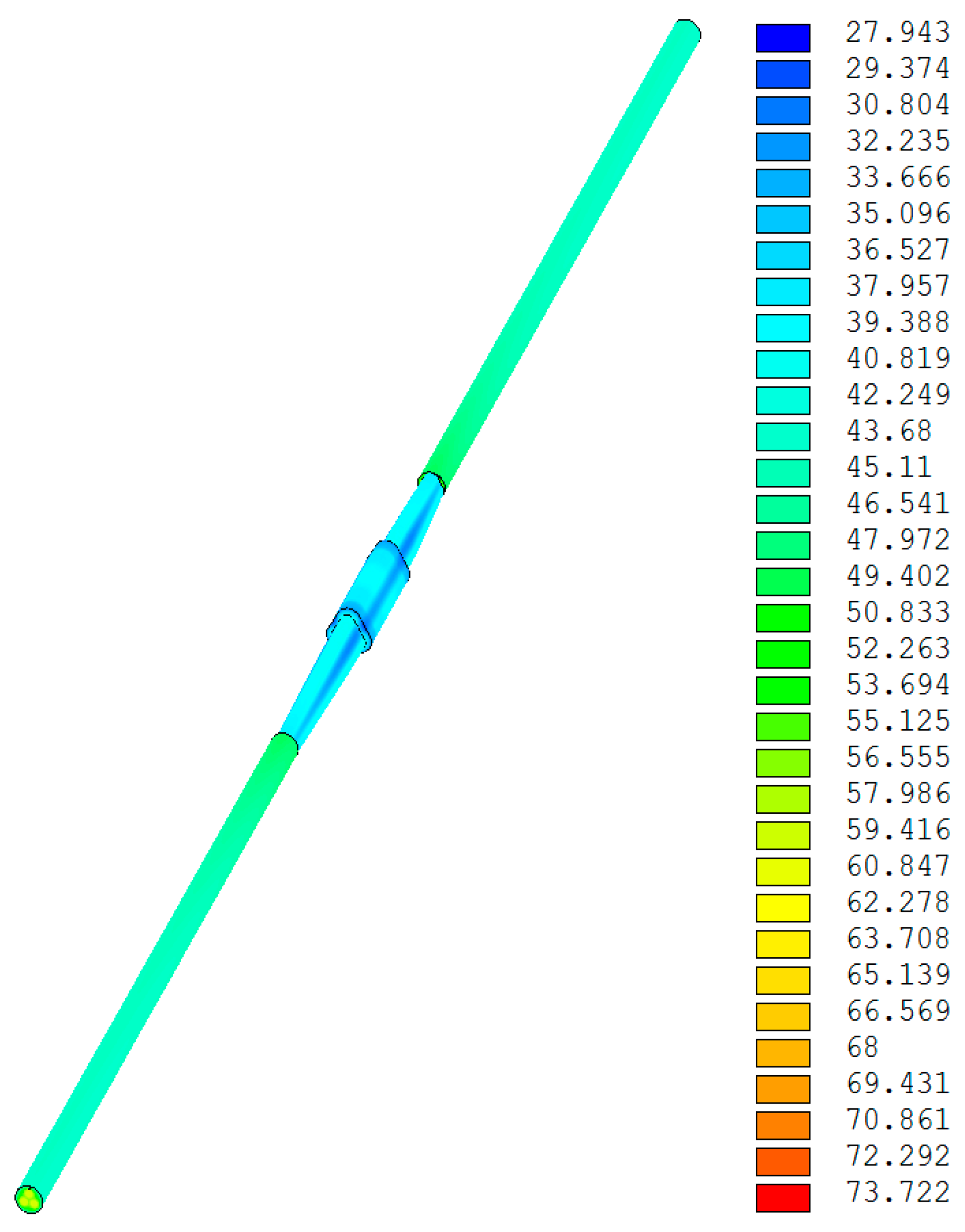
The steady-state temperature field distribution cloud map is presented in Figure 3, with a color map on the right side. Figure 3 shows that the hot spot temperature of the cable joint under this working condition is 73.722 °C, which occurs at the internal pressure connection of the cable joint. The lowest temperature is 27.943 °C, which appears at the outermost armor tape of the joint. The temperature distribution on the outer side of the armor tape is uneven and closely related to the joint structure.
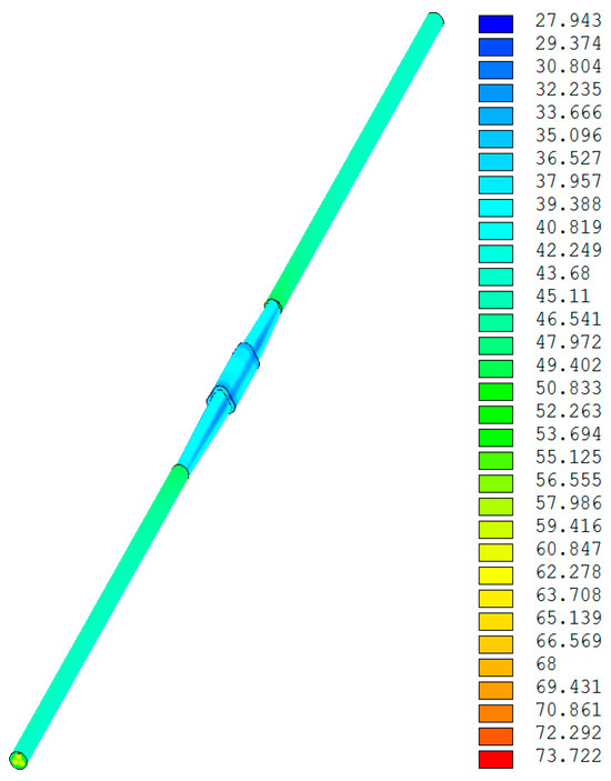
Figure 3.
Cloud map of steady-state temperature distribution of three-core cable joints (current of 500 A).
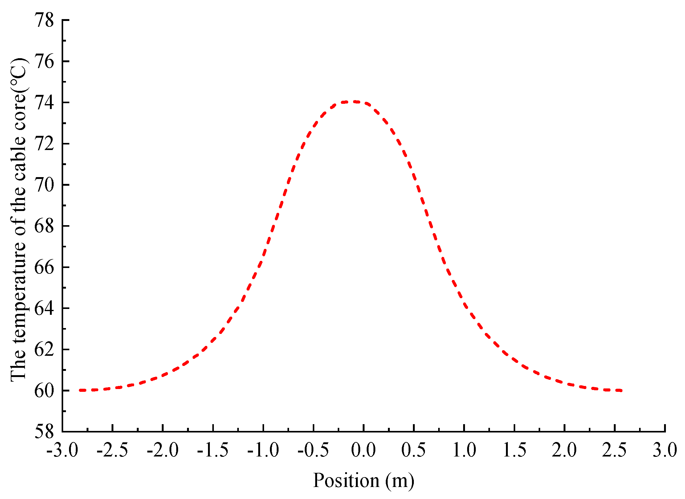
In Figure 4, the position with coordinates 0 is the center of the cable joint. For the single-phase conductor of a three-core cable, the axial temperature distribution of the conductor is approximately a Gaussian function, with high values in the middle and low values on both sides. The entire curve transitions smoothly and is significantly affected by contact resistance within 1 m from the center of the joint. The area beyond 2 m from the joint is almost unaffected by joint heat conduction.
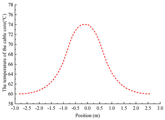
Figure 4.
Temperature distribution curve of three-core cable core.
Figure 5 shows the transient temperature rise at the cable joint pressure connection, which gradually increases from an ambient temperature of 25 °C until reaching a steady state of 73.222 °C. The temperature rise process lasted for more than ten hours, and 20 h can be approximately considered as reaching the steady-state stage.
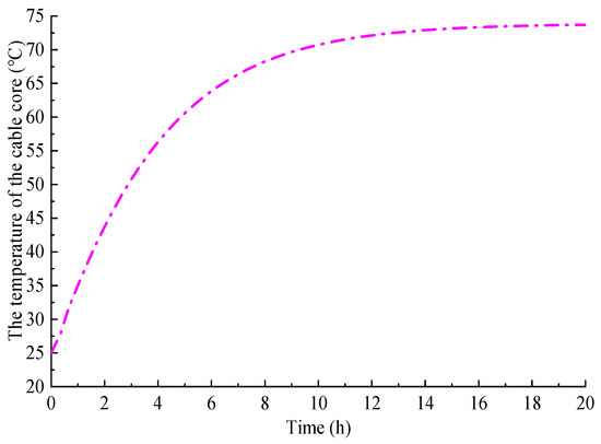
Figure 5.
Transient temperature rise curve of cable joints.
3. Temperature Inversion Method for Three-Core Cable Joints
In adherence to the heat flow diffusion principles governing the cable joint and the body, it can be deduced that two predominant flow lines exhibit distinct diffusion patterns of heat flow—namely, from the interior of the joint to the axial conductor and from the axial conductor to the outer surface [24]. Consequently, the temperature inversion methodology for 10 kV three-core cable joints encompasses two primary components. Initially, by gauging the surface temperature at various positions along the cable body, a one-dimensional transient thermal path model of the cable body was employed to deduce the corresponding temperature of the cable core at the measurement point. Subsequently, building upon the transient temperature field simulation of cable joints, a correlation was established between the contact point of the cable core within the joint and the temperature point of the cable core in the cable body. This enabled the reverse calculation of the temperature at the contact point of the cable core within the joint, commonly referred to as the hot spot temperature.
3.1. Establishment of Radial Thermal Path Model
- (1)
- Thermal resistance calculation
In the thermal circuit model, the significantly higher thermal conductivity of metal materials, in comparison to other insulation materials, results in a notable impact on temperature uniformity. Within the hot circuit, the layer containing metal acts as a crucial temperature node. Following the uniform temperature distribution of the armor layer and the symmetrical consistency of the outer sheath material, the cable’s surface temperature can be regarded as an isothermal surface, serving as another temperature node in the thermal path. Consequently, within the hot circuit, the temperature nodes progress from the innermost layer to the outermost layer, encompassing the cable core layer, metal shielding layer, armor layer, and outer sheath. The high thermal conductivity of metal materials allows their thermal resistance to be disregarded. After incorporating these considerations, the transient equivalent thermal circuit model for the three-core cable body is presented in Figure 6, while the steady-state equivalent thermal circuit model is illustrated in Figure 7.
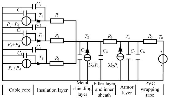
Figure 6.
Transient thermal circuit model of cable body.
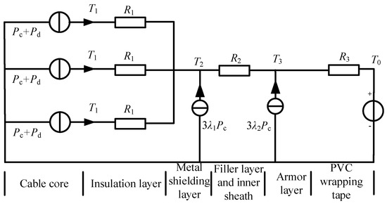
Figure 7.
Steady state thermal path model of cable body.
In the illustration, Pc and Pd denote the conductor loss and insulation medium loss of the cable core, respectively. The factors λ1 and λ2 represent the loss factors of the metal shielding layer and the armor layer, respectively. T1, T2, and T3 correspond to the temperatures of the cable core layer, the metal shielding layer, and the armor layer, respectively. T0 represents the temperature of the outer sheath, serving as an equivalent thermal pressure source. R1, R2, and R3 signify the thermal resistance of the insulation layer, the thermal resistance of the filling layer and inner sheath, and the thermal resistance of the outer sheath, respectively. C1~C6 denote the heat capacity of the conductors, insulation layer, equivalent heat capacity of the metal shielding layer, heat capacity of the filling layer and inner sheath, heat capacity of the armor layer, and outer sheath heat capacity, respectively.
Presently, the majority of 10 kV three-core cables in practical operation are of the metal belt shielding type. The thermal resistance of the insulation layer in this cable category can be computed using the following equation:
In the equation, R1 represents the thermal resistance of the cable insulation layer; R2 represents the thermal resistance of the filling layer and inner sheath; ρ1 represents the thermal resistance coefficient of the insulation layer, measured in km/W units; G represents the geometric factor of the cable; and K represents the shielding influence factor. G and K can be determined by consulting the graphical method outlined in the IEC 60287 standard [25,26].
The formula for calculating the thermal resistance of the filling layer and inner sheath is as follows:
In the formula, ρ2 is the thermal resistance coefficient of the filling material in Km/W, and G0 is the geometric factor.
The calculation formula for the thermal resistance R3 of the outer sheath is as follows:
In the formula, ρ3 is the thermal resistance coefficient of the outer sheath, in Km/W; D1 is the outer diameter of the cable, in millimeters; and D2 is the outer diameter of the armor layer, in millimeters.
- (2)
- Heat capacity calculation
The heat capacity is determined by multiplying the specific heat capacity by the mass. The heat capacity per unit length for each layer structure of a three-core cable is as follows:
In the formula, c is the specific heat capacity of the material, in J/(kg∙°C); ρ is the density of the material, in kg/m3; and V is the unit length volume of the material, in cubic meters, which is equal to the area of the cable cross-section of the structure.
In the case of each layer structure, the volume per unit length is equivalent to the cross-sectional area of the respective cable structure. With the exception of the irregularly shaped filling layer, the remaining layers can be modeled as cylindrical walls, and their heat capacity per unit length is as follows:
In the formula, ri is the outer radius of the layer material and ri−1 is the inner radius of the layer material.
3.2. Calculation Method for Axial Fitting
In practical engineering applications, the outer surface temperature of cables is relatively easy to measure, so it is necessary to establish a relationship between the outer surface temperature and the internal hot spot temperature. On the one hand, the temperature distribution pattern on the outer surface of cable joints is not obvious, and the heat conduction path is not obvious due to the influence of the material parameter dispersion. On the other hand, the transient thermal path model of the cable establishes the relationship between the external surface of the cable and the corresponding conductor temperature, and the heat transfer process is clear. In order to obtain the coupling relationship between the joint hotspot and the external surface, it is necessary to establish a fitting function between the joint hotspot temperature and the axial conductor temperature, as shown in Figure 8.
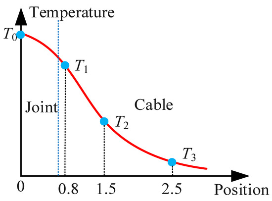
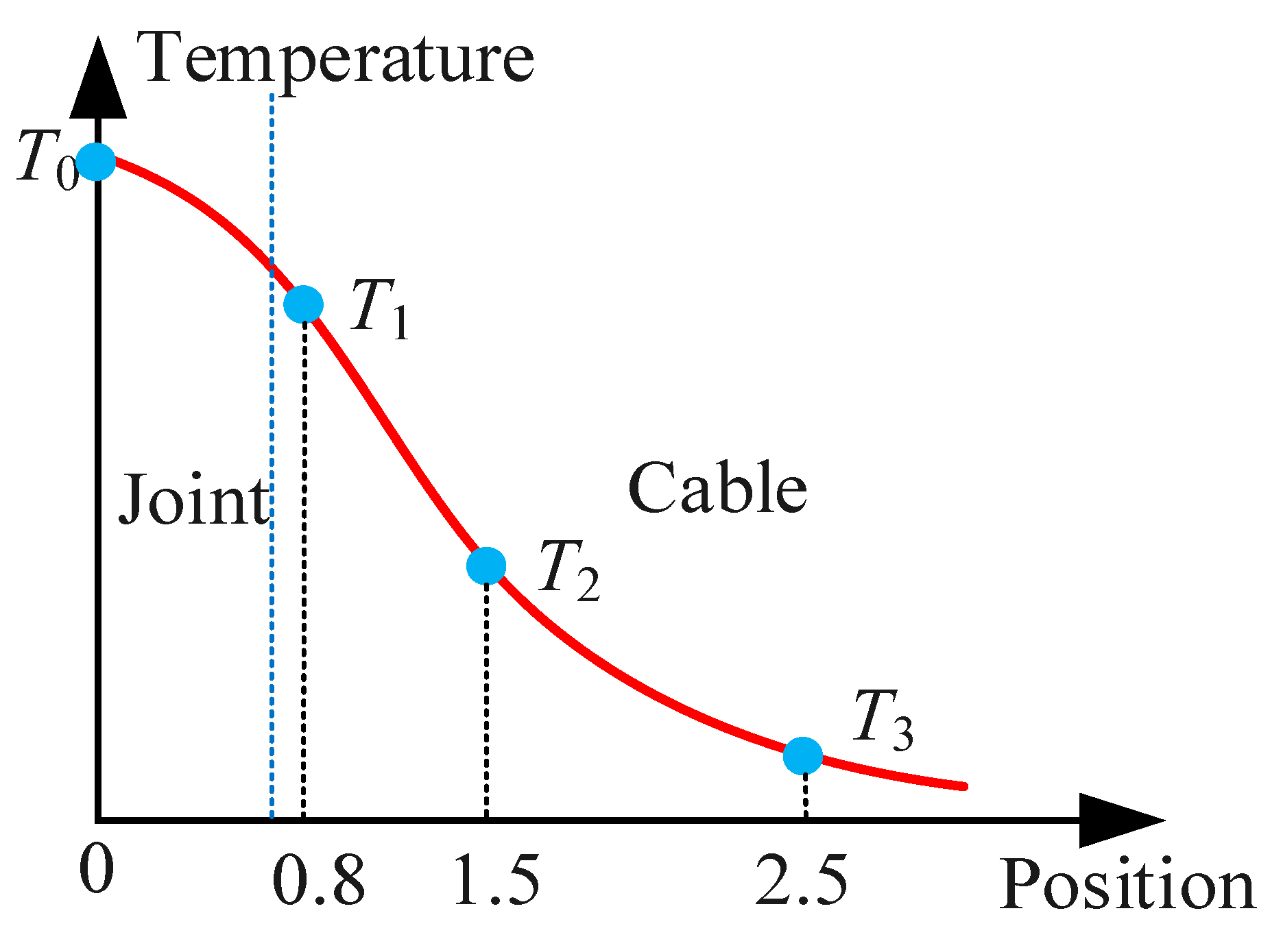
Figure 8.
Schematic diagram of axial inversion point position.
Below, a suitable expression can be formulated for the temperature (T0) at the joint crimping point and the temperatures (T1, T2, T3) at the corresponding cable core measurement points along the body. Specifically, T1 represents the temperature of the cable core corresponding to the measurement point near the joint, while T2 and T3 denote the temperatures of the cable core corresponding to measurement points farther away from the joint.
A single-step transient temperature field simulation was conducted with load values ranging from 100 A to 600 A, with each interval set at 100 A. The initial temperature and ambient temperature for each calculation were fixed at 25 °C. The convective heat transfer coefficient was established at 8 W/(m2·K). Each single-step calculation spanned a duration of 20 h, with transient result data collected every 20 min. The fitting relationship between the temperature at the crimping point of the joint and the corresponding cable core temperature at the measurement point is as follows:
The fitted mean square error (RMSE) is 0.1199, and the correlation coefficient R2 is 0.99998, indicating a good agreement between the fitted value and the original value.
4. Verification of Joint Temperature Inversion Model
4.1. Continuous Load
Maintaining a constant cable core current of 500 A for a duration of 20 h, the boundary conditions remained unchanged throughout. The temperature at the crimping point of the cable joint can be determined based on the cable skin temperature and subsequently compared with the cable joint temperature obtained through finite element simulation. The temperature rise curve at the cable crimping point is depicted in Figure 9. The findings revealed that, under a sustained load, the temperature at the joint crimping point calculated through the combination inversion method using temperature measurements on the cable body skin aligns with the trend obtained from the finite element calculations. The maximum absolute error observed was within 3 °C. The figure shows the simulation values, inversion values, and temperature differences of the hot spot temperature.
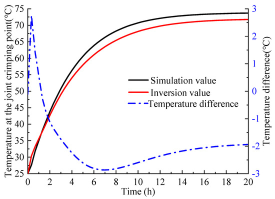
Figure 9.
Temperature rise curve at joint crimping under load.
4.2. Periodic Load
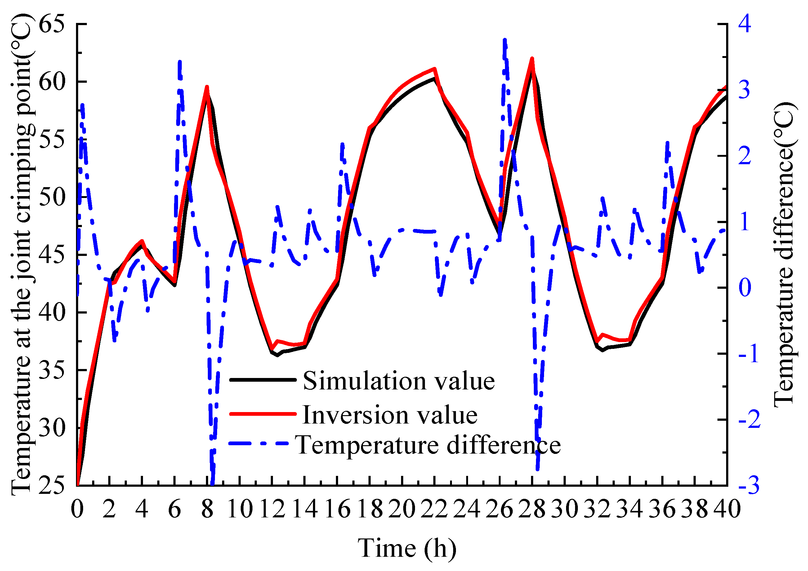
Each segment of the periodic load was maintained for a duration of 2 h, constituting a complete cycle lasting 20 h. The periodic currents followed a sequence of 100 A–600 A–500 A–400 A–300 A–600 A–200 A–100 A–300 A–400 A–550 A–500 A, respectively. Two cycles were calculated, totaling a duration of 40 h, while the boundary conditions and sustained load remained constant. The temperature rise curve at the cable crimping point is illustrated in Figure 10.
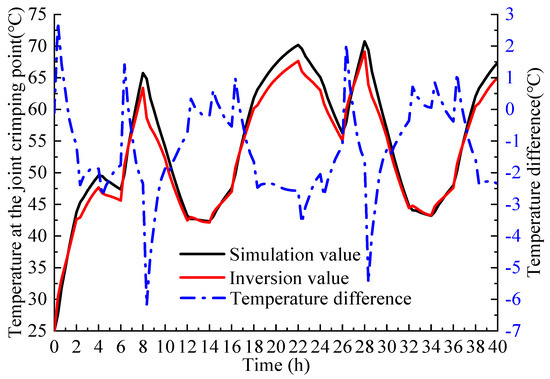
Figure 10.
Temperature rise curve at joint crimping under periodic load.
The research results indicate that under a continuous load, the temperature of the joint pressure contact calculated by the combination inversion method is consistent with the trend obtained by the finite element calculation. When the load suddenly increases or decreases, the temperature error significantly increases, with a maximum error of 6.2 K. The reason for this is that when the load changes, the heat source at the contact resistance of the joint causes a rapid change in the temperature of the hot spot. However, it takes time for internal heat to transfer to the surface, resulting in a certain lag in the surface temperature. Therefore, there is a significant difference between the hot spot temperature obtained through the surface temperature inversion and the simulation calculation results. When the load remains constant, the outer surface temperature can more accurately reflect the internal hot spot temperature, and the inversion result has a smaller error. In actual operation, the load fluctuation is relatively small, so the inversion error is also small, which can meet the actual needs of engineering.
4.3. Taking into Account the Influence of Material Parameter Dispersion
In the comprehensive model of the three-core cable joint, the primary structure remains notably stable, with the material parameters of the armor tape exhibiting a relatively significant dispersion. To assess the effectiveness of the temperature inversion method in accommodating material dispersion within the joint, the thermal conductivity of the armor tape was altered to 0.14 W/(m2∙K) while maintaining consistency in the other material parameters, load current, and boundary conditions. Subsequently, the joint temperature inversion results were calculated and compared with the finite element simulation outcomes.
The calculation results are shown in Figure 11. Comparing the simulation results in Figure 10 and Figure 11, after changing the thermal conductivity of the armor tape, the temperature of the joint crimping point significantly decreased, with the highest temperature dropping from 70.2 degrees Celsius to 60.1 degrees Celsius. The reason for this is that as the thermal conductivity increases, the heat dissipation capacity of the joint is enhanced, and the hot spot temperature decreases accordingly. When the load suddenly changes, there is a significant temperature difference between the inversion value and the simulation calculation result. As time goes on, the temperature error of the inversion value gradually decreases, and the overall temperature error is less than 3 K. In addition, this result proves that the inversion algorithm still has good adaptability after changing the joint material.
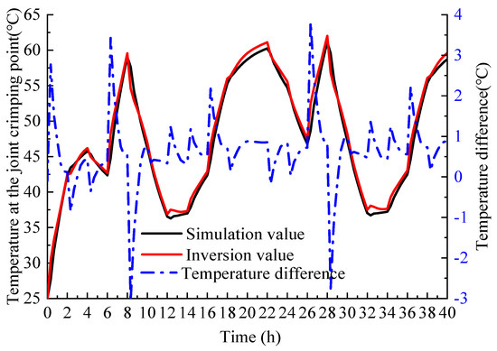
Figure 11.
Analysis of inversion effect of armor belt parameter changes.
5. Conclusions
This study established a three-dimensional finite element model of the intermediate joint of a three-core cable. When the convective heat transfer coefficient is 8 W/(m2∙K) and the surrounding air temperature is set to 25 °C, the steady-state temperature of the hottest point of the cable joint reaches 73.72 °C under a cable core current of 500 A.
In addition, a transient thermal path model of the cable body and an axial fitting function of the conductor were constructed, and the coupling relationship between the surface temperature of the body and the hot spot temperature of the joint was studied, thus developing a method for inverting the hot spot temperature of the cable joint. Under a single load, the temperature inversion results at the joint compression point showed a trend consistent with the finite element calculation results, with a steady-state error of less than 2 K. Under periodic loads, when the load suddenly increases or decreases, the temperature error significantly increases, with a maximum error of 6.2 K, which meets the requirements of practical engineering and verifies the accuracy of the proposed three-core cable joint temperature combination inversion method.
Finally, the influence of the dispersion of the cable joint material parameters was considered, and the thermal conductivity of the outermost armor tape was changed. Under periodic loads, the temperature error between the inversion results and the simulation calculation results was less than 3 K, proving that the inversion algorithm still has good adaptability after changing the joint material.
Author Contributions
Conceptualization, X.L.; methodology, Q.C. and J.R.; software, Y.M.; validation, A.H.; writing—original draft preparation, X.L., Q.C., Y.M., A.H. and J.R. All authors have read and agreed to the published version of the manuscript.
Funding
This research was funded by the National Natural Science Foundation of China (No. U2066217) and the Science and Technology Project of China Southern Power Grid Company Limited (No. GDKJXM20220135).
Data Availability Statement
Data are contained within the article.
Conflicts of Interest
Authors Xinhai Li, Qizhong Chan and Yue Ma were employed by Guangdong Zhongshan Power Supply Bureau of China Southern Power Grid Co., Ltd. The authors declare that this study received funding from China Southern Power Grid Company Limited. The funder was not involved in the study design, collection, analysis, interpretation of data, the writing of this article or the decision to submit it for publication.
References
- The National Development and Reform Commission. Guiding Opinions on Accelerating the Construction and Renovation of Distribution Networks; The National Development and Reform Commission: Beijing, China, 2015. [Google Scholar]
- Liu, G.; Lei, C.; Liu, Y. Analysis on transient error of simplified thermal circuit model for calculating conductor temperature by cable surface temperature. Power Syst. Technol. 2011, 35, 212–217. [Google Scholar]
- Guo, W.; Zhou, S.L.; Wang, L.; Pei, H.; Zhang, C.; Li, H.C. Design and application of online monitoring system for electrical cable states. High Volt. Eng. 2019, 45, 3459–3466. [Google Scholar]
- Xia, C.; Liu, H.; Wu, G.; Xia, Z. Research on the Heat Dissipation Performance and Current Carrying Capacity of the Intermediate Joint of Three Core Cables with Explosion Proof Boxes. Electr. Meas. Instrum. 2022, 59, 47–52. [Google Scholar]
- Yuan, Y.; Gao, L.; Zhu, C.; Dong, J.; Ye, Z.; Zou, H. Method for calculating the temperature of high-voltage three-core cable joints based on support vector regression. Power Supply Consum. 2023, 40, 85–91. [Google Scholar]
- Bucolo, M.; Buscarino, A.; Carlo, F.; Fortuna, L. Chaos Addresses Energy in Networks of Electrical Oscillators. IEEE Access 2021, 9, 153258–153265. [Google Scholar] [CrossRef]
- Guo, X.; Wang, Q.; He, X.; Wang, Z. Temperature Trend Simulation and System Design of Cable Conductors in Distribution Networks. Power Supply Consum. 2020, 37, 83–88. [Google Scholar]
- Lv, G.; Zhang, D.; Fu, C.; Yang, L.; Zhou, C.; Wu, X.; Liu, B. Split Conductor in Preset Temperature Fiber XLPE Cables and Accessories of the Development and Test. Electr. Wire Cable 2013, 5, 8–11. [Google Scholar]
- Lis, J.; Thelwell, M.J. Analogue investigation of water cooling of e.h.v cables. Proc. IEEE 1965, 112, 335–341. [Google Scholar] [CrossRef]
- Weedy, B.M.; Thelwell, M.J. Transient thermal performance of ehv-cable joints. Proc. IEEE 1972, 119, 472–478. [Google Scholar]
- Xu, Y.; Wang, L.; Gao, H.; Xie, X. Theoretical study on temperature field distribution of power cable joints. Power Syst. Prot. Control 2008, 36, 4–7. [Google Scholar]
- Hu, W.; Hu, Q.; Lin, X.; Lin, S. Research on Cable Joint Temperature Monitoring System Based on Temperature Field. Ind. Min. Autom. 2013, 39, 90–93. [Google Scholar]
- Lin, S.; Hu, W. Theoretical research on temperature field of power cable joint with FEM. In Proceedings of the International Conference on System Science and Engineering, Dalian, China, 30 June–2 July 2012. [Google Scholar]
- Chang, W.; Han, X.; Li, C.; Ge, Z. Experimental Study on Table Joint Temperature Measurement Technology under Step Current. High Volt. Eng. 2013, 39, 1156–1162. [Google Scholar]
- Han, X. Research on Online Monitoring System for Temperature of Intermediate Joints in Power Cables; North China Electric Power University: Beijing, China, 2012. [Google Scholar]
- Xiao, W.; Han, Q.; Zhu, W.; Zhan, Q.; Yi, S. Temperature prediction of cable joints based on generalized regression neural network. Electr. Power 2013, 32, 34–37. [Google Scholar]
- Gao, Y.; Tan, T.; Liu, K.; Ruan, J. Research on Temperature Retrieval and Fault Diagnosis of Cable Joint. High Volt. Eng. 2016, 42, 535–542. [Google Scholar]
- Chen, M. Simulation Study on Temperature Field of 10 kV Three Core Cable Joint; Xi’an University of Science and Technology: Xi’an, China, 2019. [Google Scholar]
- Yu, J. Temperature and Electric Field Simulation Analysis of 35 kV Three Core XLPE Cable Changing to Three Pole DC Operation. Electrotech. J. 2017, 8, 6–7, 49. [Google Scholar]
- Li, J.; Liu, G.; Li, L. Optimization study of thermal evaluation model for cable laying in pipeline clusters. Guangdong Electric Power. 2023, 36, 115–125. [Google Scholar]
- Li, X.; Chen, Y.; Liu, J.; Wang, X. Analysis of steady-state thermal path model for intermediate joints of 10 kV three core cables considering axial heat dissipation. Power Grid Clean Energy 2023, 39, 56–62, 69. [Google Scholar]
- Tao, W. Heat Transfer; Version 5; Higher Education Press: Beijing, China, 2019. [Google Scholar]
- Cengel, Y. Heat Transfer—A Practical Approach; Mc-Graw Hill: New York, NY, USA, 2003. [Google Scholar]
- Ruan, J.; Deng, Y.; Huang, D.; Duan, C.; Gong, R.; Quan, Y.; Hu, Y.; Rong, Q. HST Calculation of a 10 kV Oil-immersed Transformer With 3D Coupled-field Method. IET Electr. Power Appl. 2020, 14, 921–928. [Google Scholar] [CrossRef]
- IEC 60287-1-1: 2023; Electric Cables-Calculation of the Current Rating-Part 1-1: Current Rating Equations (100% Load Factor) and Calculation of Losses-General. IEC: Geneva, Switzerland, 2023.
- IEC 60287-2-1: 2023; Electric Cables-Calculation of the Current Rating-Part 2-1: Thermal Resistance-Calculation of Thermal Resistance. IEC: Geneva, Switzerland, 2023.


Disclaimer/Publisher’s Note: The statements, opinions and data contained in all publications are solely those of the individual author(s) and contributor(s) and not of MDPI and/or the editor(s). MDPI and/or the editor(s) disclaim responsibility for any injury to people or property resulting from any ideas, methods, instructions or products referred to in the content. |
© 2024 by the authors. Licensee MDPI, Basel, Switzerland. This article is an open access article distributed under the terms and conditions of the Creative Commons Attribution (CC BY) license (https://creativecommons.org/licenses/by/4.0/).