Energy Storage Capacity Configuration Planning Considering Dual Scenarios of Peak Shaving and Emergency Frequency Regulation

Abstract

New energy storage methods based on electrochemistry can not only participate in peak shaving of the power grid but also provide inertia and emergency power support. It is necessary to analyze the planning problem of energy storage from multiple application scenarios, such as peak shaving and emergency frequency regulation. This article proposes an energy storage capacity configuration planning method that considers both peak shaving and emergency frequency regulation scenarios. A frequency response model based on emergency frequency regulation combined with low-frequency load shedding is established, taking into account the frequency safety constraints of the system and the principle of idle time reuse, to establish a bi-level programming model. In the upper-level model, the optimization objective is to minimize the annual operating cost of the system during the planning period, combined with the constraints of power grid operation to plan the energy storage capacity. The lower-level model embeds frequency safety constraints with the optimization objective of minimizing the cost of fault losses. To solve the bi-level optimization problem, the Karush–Kuhn–Tucher (KKT) condition and Big-M method were used to transform the bi-level model into a single-layer linear model. Finally, an improved IEEE RTS-24 system was used for numerical verification. The results show that the method proposed in this article can reasonably plan the capacity of energy storage, improve frequency safety during system operation, and reduce the operating cost of the power grid.

1. Introduction

In recent years, in order to achieve the goals of “carbon peak” and “carbon neutrality”, a power network based on new energy has been constructed. The intermittency, volatility, and anti-peak characteristics of wind and solar power are obvious, expanding the peak valley difference and increasing the peak shaving burden of the power system [1,2]. Thermal power still dominates the power system, and it is difficult to regulate the output of thermal power units during peak shaving. Frequent start-ups and shutdowns can increase coal consumption and maintenance costs [3]. Especially during periods of low load, the downward adjustment flexibility of the power system is severely insufficient, resulting in a large amount of wind and solar power curtailment, which affects the economic efficiency of the system’s operation. New energy affects low-frequency load-shedding strategies by changing the load structure of the power grid, reducing the inertia of the power system, and reducing the frequency regulation resources of the system [4].

Energy storage has bidirectional regulation ability, fast response speed, simple control, and flexible installation position, and it can be an effective method for system peak shaving [5]. At the same time, new types of energy storage, represented by electrochemical energy storage, can provide rotational inertia for the power grid and emergency power support (EPS) for the system in a short period of time after a fault, participating in emergency frequency regulation, improving the frequency stability support ability of the power system [6]. Using battery energy storage (BES) to support frequency, the action of low-frequency load-shedding devices can be reduced, and the cost of load shedding can be reduced. Compared to traditional rotary backup technology, it has a faster response speed and can reserve frequency modulation capacity at any time, resulting in higher efficiency and reliability. If only a single application scenario is considered for energy storage configuration, ignoring the value of other auxiliary services of the grid-side energy storage power station, the benefits of energy storage will be underestimated, resulting in a mismatch between the energy storage configuration capacity in the planning and construction stage and the actual energy storage demand capacity of the system. It is difficult to fully tap the potential coordinated operation of multiple application scenarios such as energy peak shaving and frequency regulation and reduce the enthusiasm of energy storage operators to install energy storage [5]. At present, multiple countries and regions have successively constructed grid-side energy storage to participate in multi-scenario applications such as peak shaving and frequency regulation. In countries such as the United States, Australia, and the United Kingdom, grid-side energy storage is mainly used to participate in the frequency regulation market [7]. There are also many demonstration projects in China, such as the energy storage power station demonstration projects in Jinjiang, Fujian, and Changsha, Hunan, which provide peak shaving and frequency regulation services for local substations after completion; the Zhejiang Power Grid plans to develop new energy storage systems with a capacity of over 5 MW/5 MWh, enabling them to participate in peak shaving auxiliary services and provide rotating backup services [8].

At present, domestic and foreign scholars have achieved certain research results in optimizing energy storage configuration and participating in energy storage planning for peak shaving and frequency regulation applications in power systems. Reference [9] models the benefits of user-side configuration of battery energy storage arbitrage, peak shaving, frequency regulation, and other profit methods to guide energy storage configuration. Reference [10] flexibly adjusts the traditional peak shaving period for energy storage and optimizes the energy storage configuration scheme with the objective function of minimizing net cost. By incorporating primary and secondary frequency regulation energy constraints into peak shaving constraints, references [11,12] established an energy storage planning method that considers the dual constraints of peak shaving and frequency regulation. Reference [13] proposed an operational strategy for energy storage to participate in both peak shaving and frequency regulation markets, achieving a comprehensive optimization of energy storage configuration and operational efficiency. Reference [14] considers that energy storage response time is faster than traditional backup resources and establishes a specific set of peak shaving and frequency modulation scenarios. The capacity requirements of system-level energy storage are analyzed using 15 min and 5 min as the time scales for peak shaving power adjustment and frequency modulation power adjustment, respectively. However, the above energy storage frequency regulation planning method only considers energy storage as a conventional frequency regulation backup resource and does not introduce frequency safety constraints to enhance the emergency frequency regulation capability of energy storage.

The above methods focus more on the cost and benefits of the power grid without considering the system frequency response model. Establishing frequency safety constraints for energy storage to provide EPS can better unify the two demands of the power grid for energy storage peak regulation and emergency frequency regulation, fully tapping into the potential for coordinated operation of multiple application scenarios such as energy storage peak regulation and frequency regulation. Therefore, many scholars are studying frequency response models for energy storage and actively exploring the ability of energy storage for peak shaving and frequency regulation. The relevant methods are shown in

Table 1. Research on EPS and peak shaving.

References	Methods Adopted in the References
[15]	Energy storage adopts virtual droop control to participate in grid frequency stability; energy storage planning is constrained by system frequency deviation.
[16,17]	On the basis of reference [15], the influence of inertia provided by energy storage on primary frequency regulation was considered, and the influence of energy storage control parameters on frequency stability was studied.
[18,19]	The principle of “idle time reuse” was adopted, which improved the frequency of the power grid by utilizing idle energy storage during non-peak shaving stages, solving the problem of low energy storage revenue and utilization rate in single scenario applications of peak shaving.
[6]	This paper established a dynamic frequency model for the power grid, considering the improvement of energy storage on grid frequency, and established an energy storage planning model with the goal of inertia distribution and determining the total operating cost of the power system.
[20]	This paper integrated the benefits of energy storage peak shaving and frequency regulation into the same framework, expressing it as a stochastic optimization problem.

.

However, some challenges still remain.

(1) Firstly, as mentioned above, energy storage can participate in peak shaving and frequency regulation simultaneously, but even if a frequency response model for energy storage is established, it cannot reasonably represent the benefits of energy storage participating in frequency regulation and thus cannot guide energy storage planning.

(2) Secondly, traditional algorithms only evaluate energy storage configurations from a cost or benefit perspective, but doing so may lead to optimization results that are more biased towards one aspect of peak shaving or frequency modulation benefits. We need to propose an algorithm that enables energy storage to provide peak shaving and EPS for emergency frequency regulation while achieving dual objective optimization of peak shaving benefits and emergency frequency regulation benefits.

Therefore, this article proposes an energy storage capacity configuration planning method that considers the dual scenarios of peak shaving and emergency frequency regulation. The configuration problem in the dual scenarios is established as a bi-level programming model: the upper-level model solves the battery energy storage (BES) capacity configuration problem with peak shaving constraints. The lower-level model introduces established frequency constraints to address system frequency security issues. The key points of the entire text are as follows:

Section 2 derives a power system frequency response model that combines emergency frequency regulation with low-frequency load shedding provided by BES. It quantifies the benefits of BES in providing EPS with the ability to participate in emergency frequency regulation. In Section 3, based on the principle of “idle time reuse”, a bi-level programming model for BES is established to distinguish between energy storage peak shaving and emergency frequency regulation periods while also considering the benefits of peak shaving and providing EPS for emergency frequency regulation. Section 4 provides a method for solving the model, using the Monte Carlo method to extract the results of a single upper-level model to obtain fault scenarios. The bi-level model is transformed into a single-layer linear model using KKT conditions and the Big-M method for solution. Finally, in Section 5, a case study is conducted to verify the economic feasibility of BES peak shaving and emergency frequency modulation scenarios.

2. BES Emergency Frequency Regulation Combined with Low-Frequency Load Shedding for Power System Frequency Response

The frequency variation of a power system is related to real-time power balance. After an N-k fault occurs in the power system, the system power balance is disrupted, causing a change in frequency. In addition to primary frequency control by starting generator units, short-term measures to prevent frequency changes in the grid include the involvement of BES in frequency control. BES can participate in emergency frequency regulation at the millisecond level, providing virtual inertia. This section analyzes the process of BES participating in power system frequency response. Furthermore, considering the role of low-frequency load-shedding devices when the regulation capacity is exceeded, a system frequency security constraint, including low-frequency load shedding and BES providing EPS, is established.

2.1. The Power System Frequency Response after BES Provides Emergency Frequency Regulation

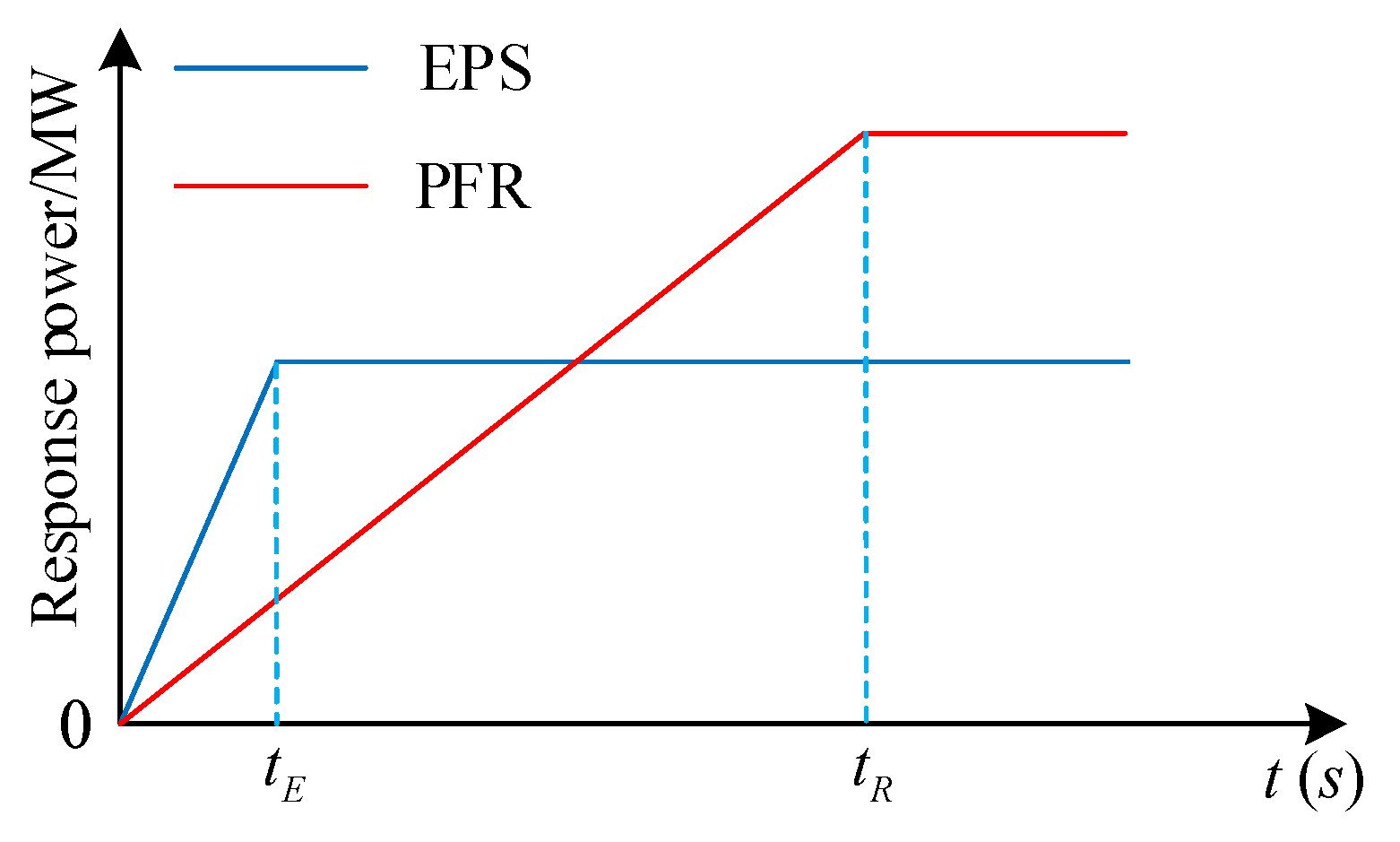
The transient frequency variation process in a power system can be divided into three stages: inertia response, primary frequency response (PFR), and secondary frequency response. Typically, the inertia response time is around 5 s, the PFR duration ranges from 5 to 25 s, while the secondary frequency response duration usually extends to several tens of minutes. This paper utilizes BES for emergency power support during the inertia response and PFR processes to improve the frequency decline rate. It is believed that in fault scenarios, reserve-generating units can provide sufficient support power during secondary frequency response. Therefore, this section analyzes the inertia response and primary frequency response processes. Through the PFR of synchronous generators and the EPS of BES, the frequency of the system decreases to the minimum point and then recovers during the quasi-steady-state process. Compared to the PFR process of synchronous generators, BES can provide millisecond-level EPS and participate in the power system inertia response. As shown in Figure 1, it should be assumed that the responses of PFR and EPS increase linearly with time and that PFR and EPS fully respond at times $t_E$ and $t_R$ respectively, as shown in Equations (1) and (2) [6,21].

$$P_{g,i}(t)=\left\{\begin{array}{cc}{P}_{g,i}t/t_R& \mathrm{if} t\le t_R\\ P_{g,i}& \mathrm{if} t>t_R\end{array}\right.,$$

(1)

$$P_e(t)=\left\{\begin{array}{cc}{P}_{e}t/t_E& \mathrm{if} t\le t_E\\ P_e& \mathrm{if} t>t_E\end{array}\right..$$

(2)

Here, $P_{g,i}$ represents the PFR capacity for synchronous unit i; $P_e$ represents the EPS capacity of BES; $P_{g,i}(t)$ represents the PFR power of synchronous unit i; $P_e(t)$ represents the EPS power of BES; $t_R$ represents the complete response time for PFR; $t_E$ represents the complete response time for EPS.

BES adopts virtual inertial control, which can simulate the working characteristics of synchronous generator sets, and the inertial time constant is often larger than that of general thermal power units. The virtual inertia of BES is related to its virtual inertia control coefficient. The total inertia of the system can be represented as follows:

$$H=\sum _i{H}_{G,i}{P}_{G,i}^{\max }{u}_i+H_E{P}_E.$$

(3)

Here, H represents the system inertia; $H_{G,i}$ represents the inertia constant of synchronous unit i; $P_{G,i}^{\max }$ represents the capacity of synchronous unit i; $u_i$ represents the on/off status of the i-th unit at time t; $H_E$ represents the inertia constant of BES; $P_E$ represents the rated power of BES.

The frequency variation process in power systems is typically described using the first-order swing equation of the rotor, as shown in Equation (4).

$$2H\frac{d\mathsf{\Delta }f(t)}{dt}+P_{L}D\mathsf{\Delta }f(t)={\displaystyle {\sum }_i{P}_{g,i}(t)}+P_e(t)-\mathsf{\Delta }P.$$

(4)

Here, $\mathsf{\Delta }f(t)$ represents the frequency deviation; D represents the load damping coefficient; $P_L$ represents the system load power; $\mathsf{\Delta }P$ represents the system’s unbalanced power.

The solution to Equation (4) yields the dynamic frequency variation of the system:

$$\mathsf{\Delta }f\left(t\right)=\frac{f_0}{2H}\left[\frac{P_g}{2t_R}{t}^2+P_e\left(t-\frac{t_E}{2}\right)-\mathsf{\Delta }Pt\right].$$

(5)

Here, $f_0$ represents the frequency reference value, $P_g={\displaystyle {\sum }_i{P}_{g,i}}$.

By solving Equation (5), we obtain the frequency minimum constraint (6) and the quasi-steady-state frequency constraint (7) as follows:

$$\left(\frac{H}{f_0}-\frac{P_e{t}_E}{4\mathsf{\Delta }{f}_{\max }}\right)P_g\ge \frac{{\left(\mathsf{\Delta }P-P_e\right)}^2{t}_R}{4\mathsf{\Delta }{f}_{\max }},$$

(6)

$$\left|\mathsf{\Delta }{f}_{\mathrm{ss}}\right|=\frac{\mathsf{\Delta }P-P_e-P_g}{D\cdot P_L}\le \mathsf{\Delta }{f}_{\mathrm{ss}}^{\max }.$$

(7)

Here, $\mathsf{\Delta }{f}_{\max }$ represents the allowable maximum frequency deviation; $\mathsf{\Delta }{f}_{\mathrm{ss}}^{\max }$ represents the allowable frequency deviation at a quasi-steady state.

2.2. Consideration of Power System Frequency Security Constraints with Low-Frequency Load Shedding

Section 2.1 analysis suggests that under non-severe faults, BES and synchronous generator PFR can ensure system frequency stability. However, it does not consider the scenario where the system experiences an N-k fault, resulting in severe active power shortage and causing the system frequency to violate constraints. When the frequency drops to the frequency setting value for low-frequency load shedding, such as 49 Hz, the safety stable control system takes action to initiate load shedding operations, preventing further deterioration. Typically, the initial action of low-frequency load shedding is set not greater than 49.5 Hz, and the duration of the system frequency below 47.5 Hz should not exceed 0.5 s, which can be used to determine the maximum frequency deviation and quasi-steady-state frequency deviation values.

In this paper, considering the occurrence of N-k faults, the frequency variation of the system is responded to by the PFR of synchronous generators and the EPS provided by BES. The portion of load exceeding the regulation capacity will be shed. To ensure that the frequency meets the requirements of the guidelines after load shedding, the shedding amount $\mathsf{\Delta }{P}_L$ is introduced to modify Equations (6) and (7), as shown in Equations (8) and (9):

$$\left(\frac{H}{f_0}-\frac{P_e{t}_E}{4\mathsf{\Delta }{f}_{\max }}\right)P_g\ge \frac{{\left(\mathsf{\Delta }P-P_e-\mathsf{\Delta }{P}_L\right)}^2{t}_R}{4\mathsf{\Delta }{f}_{\max }},$$

(8)

$$\frac{\mathsf{\Delta }P-P_e-P_g-\mathsf{\Delta }{P}_L}{D(P_L-\mathsf{\Delta }{P}_L)}\le \mathsf{\Delta }{f}_{\mathrm{ss}}^{\max }.$$

(9)

Considering that BES can provide millisecond-level EPS ($t_E$), which has negligible impact on frequency variation compared to the typical durations of 5 s for frequency deadband and 5–25 s for PFR [5], we can ignore it. Therefore, Equation (8) can be simplified to Equation (10).

$$\frac{H{P}_g}{f_0}\ge \frac{{\left(\mathsf{\Delta }P-P_e-\mathsf{\Delta }{P}_L\right)}^2{t}_R}{4\mathsf{\Delta }{f}_{\max }}.$$

(10)

3. Establishment of the Bi-Level Planning Model

In this section, a bi-level planning model is established based on a wind-thermal power system with high-penetration wind power. The model considers the system operating costs after the integration of BES for peak shaving, as well as the load-shedding losses incurred by BES participation in emergency frequency regulation under N-k fault conditions. The upper-level model aims to minimize the annual average system operating costs and incorporates typical daily operational constraints to plan the BES capacity. It is responsible for solving the BES capacity allocation problem over a long time. Within the BES configuration range provided by the upper-level decision-making, the lower-level model aims to minimize the minimum load-shedding quantity under N-k fault scenarios. It considers establishing a model for frequency security constraints in fault scenarios and is responsible for solving the emergency frequency regulation problem of BES combined with conventional primary frequency response and spinning reserve. Using the bi-level model allows for the simultaneous consideration of BES for peak shaving and emergency frequency regulation. Under the guidance of the upper-level model, BES participates in emergency frequency regulation.

3.1. Upper-Level Planning Model

• Objective function

We are considering the network operator as the operator of BES. The objective function (11) of the upper-level planning aims to minimize the total cost of system operation during the planning period after BES configuration. It includes the following components: thermal power generation cost $C_G$ (12), start-up and shutdown costs of thermal power units $C_{QT}$ (13), BES configuration and operation costs $C_E$ (14), spinning reserve costs $C_R$ (15), wind curtailment costs $C_F$ (16), and load shedding costs $C_L$ (17).

$$\min C=C_G+C_{QT}+C_E+C_R+C_F+C_L,$$

(11)

$$C_G={\displaystyle {\sum }_t{\displaystyle {\sum }_i(a_i{P}_{h,i}^2(t)+b_i{P}_{h,i}(t)+c_i)}},$$

(12)

$$C_{QT}={\displaystyle {\sum }_t{\displaystyle {\sum }_i(c_{i,t}^Q}}+c_{i,t}^T),$$

(13)

$$C_E=(c_P{P}_E+c_E{E}_E)\frac{s{(1+s)}^{T_E}}{{(1+s)}^{T_E}-1}+c_{om}{P}_E,$$

(14)

$$C_R=c_B{\displaystyle {\sum }_t{P}_G(t)},$$

(15)

$$C_F=c_F{\displaystyle {\sum }_t\mathsf{\Delta }{P}_F(t)},$$

(16)

$$C_L=\min c_L{\displaystyle \sum _{i=1}^N{p}_i}\mathsf{\Delta }{P}_{Li}.$$

(17)

Here, $P_{h,i}(t)$ represents the output of thermal power unit i at time t; $a_i$, $b_i$, and $c_i$ are the quadratic, linear, and constant coefficients of the fuel consumption characteristic function of thermal power unit i; $c_{i,t}^Q$ represents the start-up cost of unit i at time t; $c_{i,t}^T$ represents the shutdown cost of unit i at time t; $c_P$ represents the cost of BES per unit power configuration; $c_E$ represents the cost of BES per unit capacity configuration; $c_{om}$ represents the operating cost of BES per unit power; $E_E$ represents the capacity configuration of BES; $T_E$ represents the service life of BES; s represents the investment discount rate calculated at the annual interest rate; $c_B$ represents the cost of spinning reserve per unit power; $P_G(t)$ represents the spinning reserve capacity retained at time t; $\mathsf{\Delta }{P}_F(t)$ represents the curtailed wind power at time t; $c_F$ represents the wind curtailment penalty factor; $c_L$ represents the cost of load shedding per unit power; N represents the total number of generated fault scenarios; $p_i$ represents the probability of fault scenario i occurring; $\mathsf{\Delta }{P}_{Li}$ represents the amount of load shedding under fault scenario i.

2.

Constraint condition

(1) Power balance constraints

$${\displaystyle \sum _{i=1}^{N_h}{u}_i(t)P_{h,i}(t)}+P_F(t)+P_{ef}(t)=P_L(t).$$

(18)

Here, $N_h$ represents the total number of thermal power units; $P_F(t)$ represents the wind power at time t; $P_{ef}(t)$ represents the peak shaving power of BES at time t.

(2) BES capacity constraints

$$\left\{\begin{array}{l}-P_E\le P_{ef}(t)\le P_E\\ E_e(t)=E_e(t-1)-P_{ef}(t)\\ 0\le E_e(t)\le E_E\end{array}\right..$$

(19)

Here, $E_e(t)$ represents the remaining power of BES at time t. On a time scale of one day, it is considered that the capacity released by BES peak shaving is equal to the capacity absorbed by valley shaving. This is the daily energy-clearing constraint for energy storage.

(3) Peak shaving period constraints

This paper adopts the viewpoints of references [17,18] and adopts the principle of “idle time reuse” to divide the BES operation period, avoiding conflicts between the BES peak shaving period and the period used as emergency frequency regulation backup. The BES adopts the “two releases and one charge” method, with 23:00–6:00 as the peak shaving period, 9:00–14:00 and 17:00–20:00 as the peak shaving period, and the remaining periods of BES serve as rotating backup to cope with N-k faults. As shown in Equation (20), the peak shaving power of BES during the standby period is 0.

$$P_{ef}(t)=0,t\in T.$$

(20)

Here, T represents the frequency modulation backup period.

(4) Thermal power units’ constraints

$$\left\{\begin{array}{l}{P}_{G,i}^{\min }\le P_{h,i}(t)\le P_{G,i}^{\max }\\ -r_{i,d}\le P_{h,i}(t)-P_{h,i,}(t-1)\le r_{i,u}\\ [u_i(t)-u_i(t+1)][T_{h,i}^{\mathrm{on}}(t)-T_{h,i,\min }^{\mathrm{on}}]\ge 0\\ [u_i(t+1)-u_i(t)][T_{h,i}^{\mathrm{off}}(t)-T_{h,i,\min }^{\mathrm{off}}]\ge 0\end{array}\right..$$

(21)

Here, $P_{h,i,\min }$ represent the lower output limits of thermal power unit i, respectively; $r_{i,u}$ and $r_{i,d}$ represent the maximum upward and downward ramping rates of thermal power unit i, respectively; $T_{h,i}^{\mathrm{on}}(t)$ and $T_{h,i}^{\mathrm{off}}(t)$ represent the duration of start-up and shutdown of thermal power unit i, respectively; $T_{h,i,\min }^{\mathrm{on}}$ and $T_{h,i,\min }^{\mathrm{off}}$ represent the minimum duration of start-up and shutdown of thermal power unit i, respectively.

3.2. Lower-Level Planning Model

• Objective function

The objective function (23) of the lower-level planning aims to minimize the mathematical expectation of the total load shedding cost after the occurrence of N-k faults in power generation units during the planning period after BES configuration.

$$\min C_L=c_L{\displaystyle \sum _{i=1}^N{p}_i}\mathsf{\Delta }{P}_{Li}.$$

(22)

2.

Constraint condition

The variables of the lower-level model include EPS power, PFR power, and load-shedding power for each scenario. When solving the lower-level model, the constraints of BES EPS power and PFR power for spinning reserve need to be satisfied, in addition to meeting the constraints imposed by the upper-level optimization model. In other words, the EPS power and PFR power for the spinning reserve in the lower-level model will be constrained by the configuration of BES power and spinning reserve in the upper-level model.

(1) EPS power constraint

$$0\le P_{e,i}\le P_E.$$

(23)

Here, $P_{e,i}$ represents the EPS power under fault scenario i.

(2) PFR power constraint

$$0\le P_{i,g}\le P_G.$$

(24)

Here, $P_{i,g}$ represents the PFR power under fault scenario i.

(3) System frequency security constraints

System frequency security constraints also include the total system inertia constraint (3), quasi-steady-state frequency constraint (9), and frequency minimum constraint (10), which are used to determine the amount of load shedding in the scenarios. These constraints are not repeated here.

4. The Solution Method for the Bi-Level Model

The upper-level optimization model constructed in Section 2.1, after removing the objective function terms of rotational reserve cost and load shedding cost, has a separate objective function and constraint conditions that can form a typical intra-day optimization scheduling model for BES participating in peak shaving. Moreover, the operation of units outside the peak shaving period is less affected by BES configuration. Therefore, the upper-level planning model can be solved separately first to obtain the operating status of the system during the rotational backup period provided by BES. During non-peak shaving periods, the Monte Carlo method is used to sample the fault combinations of units, and the N-k (k ≤ 2) fault set of units is extracted as the fault scenario set of the lower-level optimization model to ensure robustness against parameter uncertainty.

In the bi-level model constructed in this paper, a coupling relationship exists between the upper and lower-level models, making direct solutions challenging. The solution method provided in reference [22] is adopted, where the Lagrangian function of the lower-level model is constructed, and its Karush–Kuhn–Tucker (KKT) conditions are written and substituted into the upper-level model, transforming the lower-level model into constraints of the upper-level model. This transforms the bi-level model into a single-level model. The KKT condition is necessary for low-order models to have extreme points. Solving its KKT condition will inevitably lead to extreme points in the lower-level model. Bringing it into the upper-level model inevitably leads to finding the extreme points of the upper-level model, thereby obtaining the global optimal value. Then, the Big-M method is utilized to linearize the complementary slackness conditions in the KKT conditions of the lower-level model. Additionally, constraint (10) in the lower-level model is a nonlinear constraint, which is linearized using the piecewise linearization (PWL) method [23]. This method has a shorter solving time compared to other optimization methods.

5. Case Study

This article analyzes the method proposed using an improved IEEE RTS-24 system. The improved IEEE RTS-24 system consists of 24 nodes and 12 units. The parameters of the units are listed in

Table 2. The parameters of the units.

Unit Numbers	a/(10−3 USD/MWh2)	b/(USD/MWh)	c/USD	Pmin/MW	Pmax/MW	${\mathit{r}}_{\mathit{i},\mathit{u}}$$, {\mathit{r}}_{\mathit{i},\mathit{d}}$/(MW/h)	${\mathit{c}}_{\mathit{i},\mathit{t}}^{\mathit{Q}}$$, {\mathit{c}}_{\mathit{i},\mathit{t}}^{\mathit{T}}$/USD	Forced Outage Rate
1	\	\	\	0	800	\	\	\
2, 3, 4, 5	3.5	17.5	2100	50	100	40	6000	0.05
6, 7, 8	11.6	2.1	6722	140	197	50	18,000	0.06
9, 10	70	0.91	8869	190	260	60	40,000	0.04
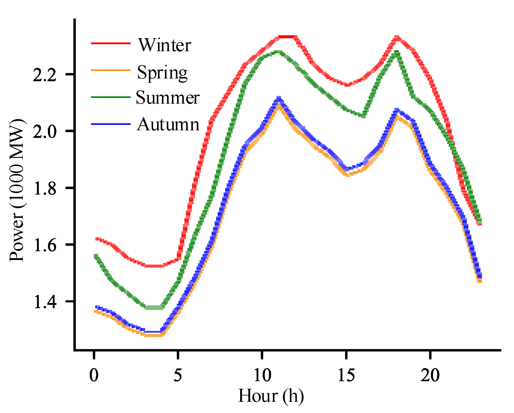
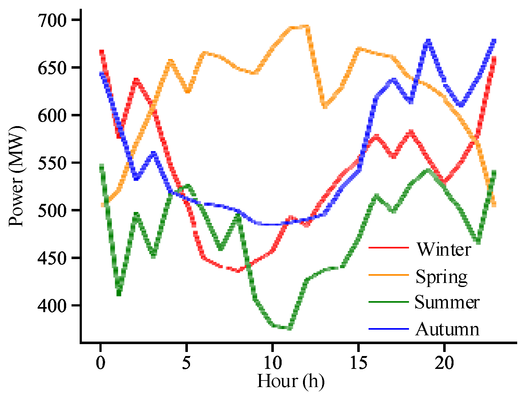
11, 12	1.4	2.87	9513	280	300	\	50,000	0.02

, where the unit with the number 1 is a wind power unit. Four typical days are selected from the year, representing winter, spring, summer, and autumn. The load data for the typical days are shown in Figure 2, while the wind power output data for the typical days are shown in Figure 3. The parameters of the BES are listed in

Table 3. Relevant parameters of BES.

Parameter Name	Parameter Value
$c_P$/(USD/MWh)	100,000
$c_E$/(USD/MW)	200,000
$c_{om}$/(USD/MW)	20
s	8%
$T_E$/year	10

. The BES capacity is set to be multiples of 10, and the virtual inertia of BES is taken as 5 s [5]. The wind curtailment penalty is set to USD 100/MWh, and the load shedding penalty is USD 1,000,000/MW. The reference frequency is set to 50 Hz, with an allowable maximum frequency deviation of 2.5 Hz and a quasi-steady-state frequency deviation of 0.2 Hz. The spinning reserve cost is set to USD 5/MWh. The proposed method is implemented using the Python compiler in Visual Studio Code and utilizes the commercial solver Gurobi-10.0.1 for solving.

To verify the effectiveness of the proposed method, this section sets up four case studies with different factors for comparative analysis. To simplify calculations, in Case 1, Case 2, and Case 3, it is assumed that the system’s spinning reserve for each time period is 10% of the load for that period [2].

Case 1: BES is not planned in the system, and during faults, only the PFR capability of the conventional spinning reserve is relied upon for regulation.

Case 2: Only peak shaving demand is considered for BES configuration using a single-layer model. The objective function does not include load-shedding costs, but BES still participates in emergency frequency regulation.

Case 3: Only emergency frequency regulation demand is considered for BES configuration, assuming that the configuration of the conventional spinning reserve is not affected. A single-layer model is used, with the objective function including only load shedding costs and BES configuration costs. It is assumed that the BES’s capacity is at least twice the BES’s power, and it does not participate in peak shaving.

Case 4: Both peak shaving demand and emergency frequency regulation demand are considered for BES configuration, taking into account the alternative role of conventional spinning reserve. The proposed bi-level model is used, and the method proposed in Section 3 is applied for solving.

The proposed method is used to solve the scenarios of Case 1 to Case 4, and the obtained BES configuration schemes and operational results are compared, as shown in

Table 4. BES configuration and typical daily operation results under different planning schemes.

Case Numbers	BES Power/MW, BES Capacity/MWh	Generation Cost/USD	Unit Start-up/Shutdown Cost/USD	Wind Curtailment Cost/USD	Load Shedding Cost/USD	Reserve Cost/USD	Total Cost/USD
Case 1	\	4.73 × 108	4 × 107	4.24 × 106	1 × 107	3.31 × 106	5.3055 × 108
Case 2	120, 260	4.62 × 108	3.24 × 107	4.41 × 105	4.57 × 106	3.31 × 106	5.1109 × 108
Case 3	160, 320	4.73 × 108	4 × 107	4.24 × 106	2.56 × 106	3.31 × 106	5.3386 × 108
Case 4	180, 530	4.56 × 108	3.55 × 107	0	1.89 × 106	1.77 × 106	5.098 × 108

.

5.1. Analysis of BES Peak Shaving Scenario Case Study Results

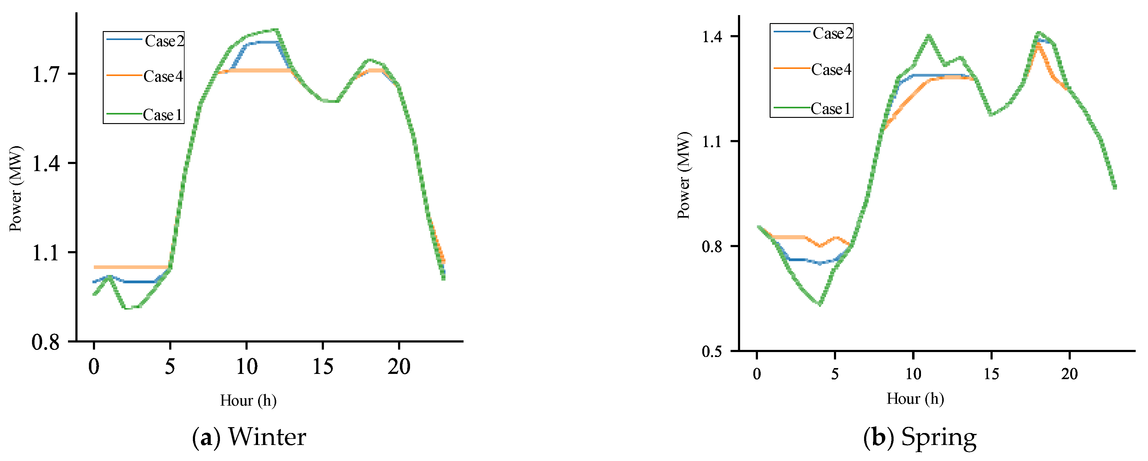
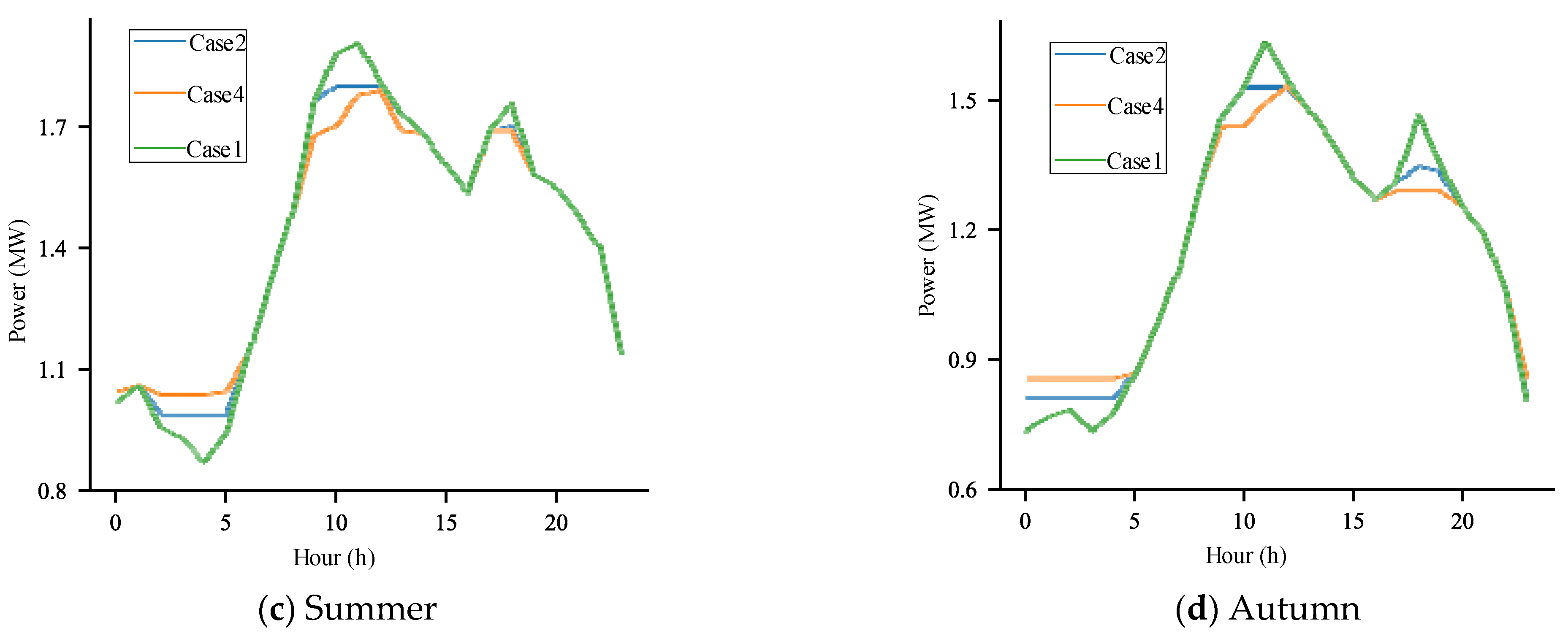
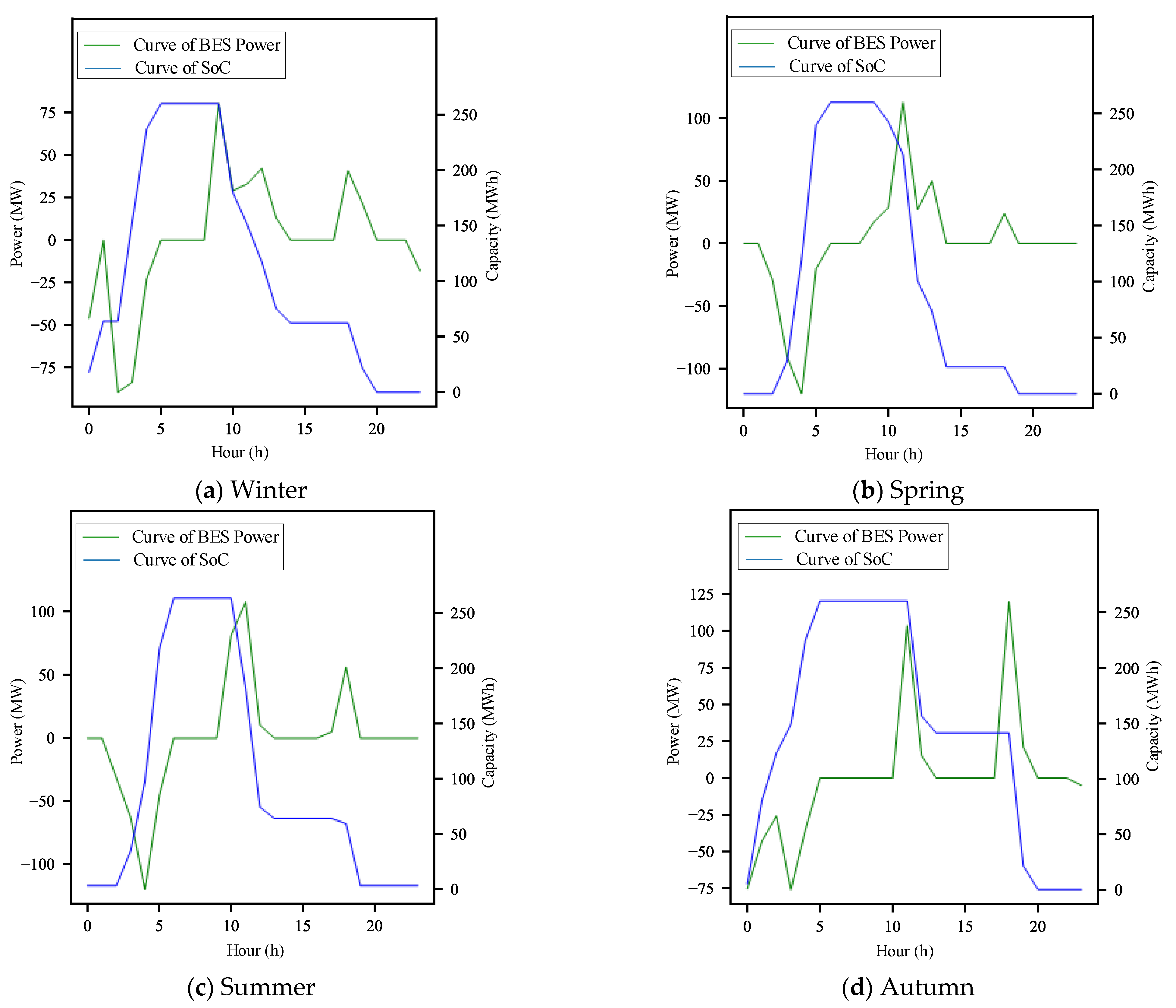
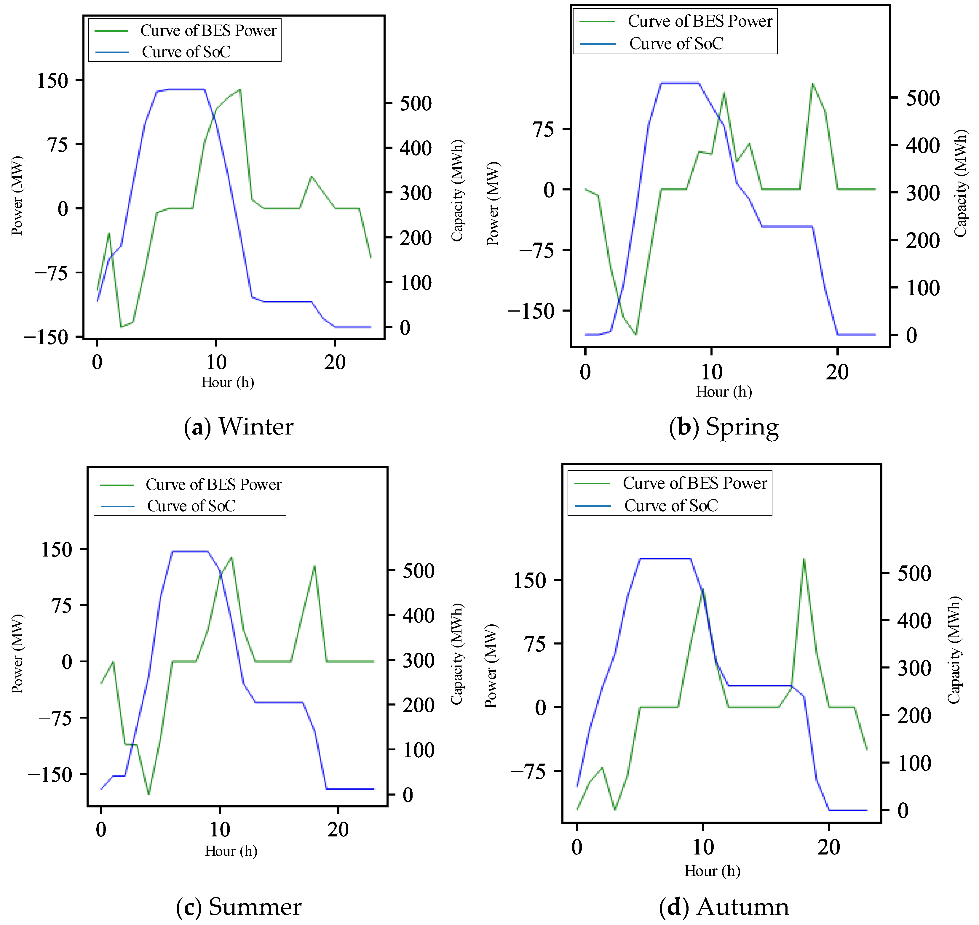
To compare the impact of BES planning results on scenarios involving both peak shaving and emergency frequency regulation and scenarios involving only peak shaving, we analyze Cases 1, 2, and 4. The comparison of net load curves between Case 1 and Cases 2 and 5 is shown in Figure 4, while the BES power and state of charge (SoC) status are illustrated in Figure 5 and Figure 6, respectively. Figure 4, Figure 5 and Figure 6 show that the BES charges during periods of low load and discharges during periods of high load, achieving the goals of integrating wind power and smoothing the output of thermal power units.

From Table 4, it is evident that Case 1, where no BES is configured, has significantly higher generation, wind curtailment, and start-up/shutdown costs compared to the other cases. In Case 2, considering the economic benefits of peak shaving and configuring BES with a power of 120MW, the grid’s generation cost decreased by 2.3%, start-up/shutdown cost decreased by 19%, and wind curtailment cost decreased by 89.6%, resulting in a total cost reduction of 3.7%. In Case 4, considering both BES emergency frequency regulation and its role as an alternative to spinning reserve, the configuration of BES is less conservative, resulting in a BES power of 180MW. Although the reduction in start-up/shutdown costs is 11.25% less than in Case 2, the total cost reduction is 3.9%.

Table 5. Typical daily operation results of Case 1.

Typical Day	Winter	Spring	Summer	Autumn
Generation cost/USD	1.36 × 108	9.87 × 107	1.34 × 108	1.08 × 108
Unit start-up/shutdown cost/USD	1.08 × 107	7.56 × 106	1.08 × 107	1.08 × 107
Peak-to-valley ratio	34.9%	39.2%	40%	39.2%
Wind curtailment cost/USD	4.41 × 105	2.14 × 106	9.36 × 105	7.2 × 105

,

Table 6. Typical daily operation results of Case 2.

Typical Day	Winter	Spring	Summer	Autumn
Generation cost/USD	1.35 × 108	8.99 × 107	1.33 × 108	1.04 × 108
Unit start-up/shutdown cost/USD	8.64 × 106	6.48 × 106	8.64 × 106	8.64 × 106
Peak-to-valley ratio	33%	34.7%	35.6%	34.4%
Wind curtailment cost/USD	0	86153	3.55 × 105	0

and

Table 7. Typical daily operation results of Case 4.

Typical Day	Winter	Spring	Summer	Autumn
Generation cost/USD	1.35 × 108	8.95 × 107	1.29 × 108	1.02 × 108
Unit start-up/shutdown cost/USD	7.88 × 106	6.48 × 106	1 × 107	1.06 × 107
Peak-to-valley ratio	32.5%	33.3%	33.8%	32.4%
Wind curtailment cost/USD	0	0	0	0

present the operational results of different typical days for Case 1, Case 2, and Case 4, respectively. The following can be observed:

(1) On typical summer and autumn, the start-up/shutdown costs of Case 2 are significantly higher than those of Case 4. This is because conventional thermal power units are set to generate electricity at higher costs during periods of low demand. On typical days with high wind penetration rates, the thermal power units increase their start-up/shutdown frequency to minimize generation costs while accommodating wind power. However, the sum of generation costs and start-up/shutdown costs is still lower in Case 4.

(2) Compared to Case 1, Case 2 with BES configuration can almost fully accommodate wind power. In contrast, Case 4 not only reduces generation costs and fully integrates wind power but also further reduces the peak-to-valley ratio. This indicates that rational planning of BES participation in peak shaving and emergency frequency regulation can allow for more BES participation in peak shaving compared to scenarios without considering emergency frequency regulation, thereby providing significant economic benefits for grid operations.

5.2. Analysis of BES Participation in Emergency Frequency Regulation Scenario Case Study Results

To compare the impact of BES participation in both peak shaving and emergency frequency regulation scenarios with only emergency frequency regulation scenarios on BES planning results, we analyze Cases 1, 2, 3, and 4. According to Table 4, if only considering BES participation in emergency frequency regulation, Case 3 with a BES configuration of 160 MW reduces the load shedding cost to 25.6% of Case 1 and 44% of Case 2 under the fault scenarios considered in this study. However, in Case 2, the load shedding cost already decreased to 45.7% of Case 1. The reduced load-shedding cost cannot offset the BES configuration and operation costs, leading to an increase in the total cost. It can be seen that considering only grid peak shaving demand or emergency frequency regulation demand for BES planning cannot fully utilize the capabilities of BES in peak shaving and emergency frequency regulation. The economic performance of only configuring BES for emergency frequency regulation is poor, resulting in an increase in the total operating cost of the grid. Therefore, it is necessary to properly represent the roles of BES in both capabilities in the planning objectives and to use the bi-level model of Case 4 for planning.

Figure 7 illustrates the comparison of load shedding among five different N-k contingency scenarios, with power deficits of 241 MW, 206 MW, 358 MW, 300 MW, and 450 MW, respectively. It can be observed from Figure 7 that the load shedding in Case 4 is significantly lower than that in Case 3, indicating better peak shaving benefits and system security in Case 4.

The analysis of Case 1 to Case 4 demonstrates that embedding frequency security constraints into BES planning, considering the frequency variation process after unit faults, can effectively assess the system’s urgent frequency regulation requirements and enhance the overall system’s frequency support capability. Incorporating wind curtailment penalties and unit start-up/shutdown costs into the objective function can effectively measure the system’s peak shaving requirements and reduce the overall system’s peak-to-valley difference. Moreover, using a bi-level model can appropriately represent the benefits of BES for both peak shaving and emergency frequency regulation, ensuring the economic operation of the system and the safety of load shedding in fault scenarios.

6. Conclusions

This paper addresses the problem of grid-side BES configuration for providing spinning reserve and peak shaving services. A capacity planning method considering both peak shaving and emergency frequency regulation scenarios is proposed, and its effectiveness is verified through case studies. The main conclusions obtained are as follows:

(1) Compared to traditional energy storage planning methods focusing solely on peak shaving and frequency regulation, this paper considers the emergency frequency regulation capability of BES during planning, ensuring frequency security in the event of N-k faults. By introducing load-shedding costs and load-shedding amounts into the upper and lower layers of the BES planning model and adding frequency constraints to the constraints, the BES planning capacity of the system is increased.

(2) BES providing emergency frequency regulation services and participating in peak shaving can effectively reduce the operating costs of the system, decrease system fault losses and conventional spinning reserve configuration costs, and improve the economic and operational security of the grid.

(3) The bi-level model algorithm proposed in this paper generally outperforms the single-layer model considering a single scenario in most economic indicators. It provides a method for evaluating the value of energy storage in providing ancillary services, which can be extended to various energy storage planning scenarios, such as pumped hydro storage and compressed air energy storage.

The bi-level planning model proposed in this paper does not consider the impact of fault duration and BES discharge time. It assumes that BES emergency frequency regulation can continuously provide power support during the fault duration. However, whether the BES’s capacity can withstand long-term power support or even participate in secondary frequency regulation requires further study. Additionally, as independent energy storage operators have gradually emerged in recent years, future models could consider the costs and benefits of independent energy storage operators to guide the economic optimization of individual energy storage systems.