Long-Term Ampacity Prediction Method for Cable Intermediate Joints Based on the Prophet Model

Abstract

The development of power grids is hindered by the limited transmission capacity of cable equipment, necessitating the accurate prediction of dynamic ampacity for cable expansion. This study focuses on the 110 kV cable intermediate joint, employing radial and axial inversion techniques for real-time conductor temperature inversion. Utilizing the Prophet time series model, we predict environmental changes and propose a dynamic ampacity evaluation method for cable intermediate joints. Experimental validation confirms the model’s accuracy, with prediction errors under 10 K, demonstrating its potential for enhancing cable system reliability and power grid development.

1. Introduction

In the realm of power systems, the integrity and reliability of cable systems are paramount. One of the most prevalent issues in this context is the overheating of cable intermediate joints, which often leads to insulation breakdown and system failure. This overheating is primarily attributed to poor conductor contact, resulting in a vicious cycle of abnormal heating. The concealed nature of the conductor within the joint further complicates the detection of such overheating, making traditional monitoring methods inadequate. Thus, there is a pressing need to develop sophisticated methods for sensing the internal heating state of cable intermediate joints, facilitating the online detection of hotspot temperatures and providing early warnings of potential overheating faults.

Moreover, the insufficient transmission capacity of cable equipment has emerged as a significant bottleneck in the development of power grids, particularly in China. The growing disparity between power supply and demand necessitates an urgent enhancement of cable equipment capacity. A critical aspect of this enhancement is the accurate prediction of dynamic ampacity, which must be both real-time and rapid to accommodate the variability of environmental conditions and the unpredictability of emergency loads.

The detection of cable conductor temperature can be broadly classified into the following two categories: implantable and non-implantable temperature measurement methods. Implantable methods, as discussed in references [1,2], involve pre-installing temperature-measuring optical fibers inside the cable’s segmented conductors during manufacturing. This approach allows for the precise measurement of the actual operating temperature of the cable conductors. However, it is not only complex in its implementation, but also inapplicable to cable circuits already in operation, posing potential safety hazards. On the other hand, non-implantable methods encompass techniques such as the thermal circuit model method, the numerical calculation method, and the experimental data mining method. A notable example of the thermal circuit model method is presented in reference [3,4], which employs a thermal resistance/capacitance equivalent network to analyze transient conductor temperature changes in tunnel-type cross-linked polyethylene cable joints. Despite these advancements, most studies using numerical calculation methods, as cited in references [5,6,7,8,9,10,11,12,13], are limited to steady-state analysis and do not adequately address the real-time online monitoring of joint hotspot temperatures.

In the realm of dynamic ampacity evaluation, various methodologies have been explored. Reference [14] employs an analytical method that incorporates the dynamic process into the transient thermal equilibrium equation of the cable to determine dynamic ampacity. Reference [15] utilizes the thermal circuit model method, drawing parallels between the temperature field and the electric field to convert the heat transfer problem into a thermal circuit model for calculation. Another approach, as demonstrated in reference [16], leverages historical data analysis using the chaotic time series Volterra method, based on singular value decomposition to predict dynamic ampacity. Despite these advancements, implantable temperature measurement technology, while offering high accuracy, introduces safety hazards when sensors are placed at high-potential conductors. Non-implantable temperature measurement technology, on the other hand, requires extensive transient computation and still falls short in industrial applications. Furthermore, most current studies on dynamic ampacity prediction rely on steady-state thermal equilibrium equations, which fail to account for the transient process of temperature rise, leading to significantly lower predicted ampacity in real-world scenarios.

This paper aims to address these challenges by focusing on the 110 kV cable intermediate joint. We construct paths for radial inversion of the body and axial inversion of the conductor, enabling the real-time inversion of conductor temperature. Utilizing the inversion results and cable surface temperature measurement information, we employ the PROPHET time series model analysis method to predict environmental changes. We propose a dynamic ampacity evaluation method for cable intermediate joints and validate it through a designed dynamic ampacity experiment.

By tackling the issues in temperature detection and dynamic ampacity prediction, this study seeks to enhance the reliability and efficiency of cable systems in power networks, contributing to the overall stability and development of the power grid.

This study focuses on the dynamic ampacity prediction for cable intermediate joints. While our research might seem unrelated to renewable energy technologies such as hydrogen fuel cells and lithium-ion batteries at first glance, the development of these technologies is crucial for the stability and efficiency of power systems. Recent studies have shown that improved membrane materials and electrode structures can significantly enhance the performance of these energy storage and conversion devices [17,18]. Similarly, this study aims to contribute to the reliability and efficiency of power systems by accurately predicting the dynamic ampacity of cable intermediate joints.

2. Inversion Model for Hotspot Temperature of Cable Intermediate Joints

Predicting the dynamic ampacity of cable systems is a critical aspect of ensuring their reliability and efficiency in power networks. A key factor in this prediction is the accurate determination of hotspot temperatures within cable intermediate joints. These hotspots, if not properly managed, can lead to insulation breakdown and system failures. Therefore, developing an inversion model for hotspot temperature is essential for assessing the thermal performance of cable joints and, subsequently, for accurately predicting their dynamic ampacity.

Accurate prediction of hotspot temperatures in cable intermediate joints is crucial for ensuring the reliability and safety of power systems. The inversion model for hotspot temperature is a vital component of this prediction, consisting of two main parts, as follows: radial inversion of the body and axial inversion of the conductor.

Radial Inversion of the Body: This process involves using surface temperatures, T_s1 and T_s2, as inputs to calculate the corresponding body conductor temperatures, T₁ and T₂, through a transient thermal circuit model, as shown in Figure 1. T_s1 is located 0.2 m from the end of the joint, close enough to reflect its influence, while T_s2 is 2.2 m away, far enough to capture the body’s impact. The radial inversion of the body is crucial for accurately determining the temperature distribution within the cable joint. This step is based on the assumption that the thermal properties of the materials involved are homogeneous and isotropic and that heat transfer occurs primarily through conduction. The model also assumes that the joint’s geometry and material properties are known and that the surface temperatures are representative of the temperatures within the joint.

Axial Inversion of the Conductor: After obtaining T₁ and T₂ from the radial inversion, these values are used as inputs for an axial temperature inversion function. This function is constructed using transient temperature field simulation data as training samples, which allows us to determine the joint’s hotspot temperature, T_j. The axial inversion of the conductor is based on the assumption that the temperature distribution along the conductor’s axis can be accurately modeled using the available simulation data. This part of the model is crucial for assessing the thermal performance of the cable joint and identifying potential hotspots that could lead to failures.

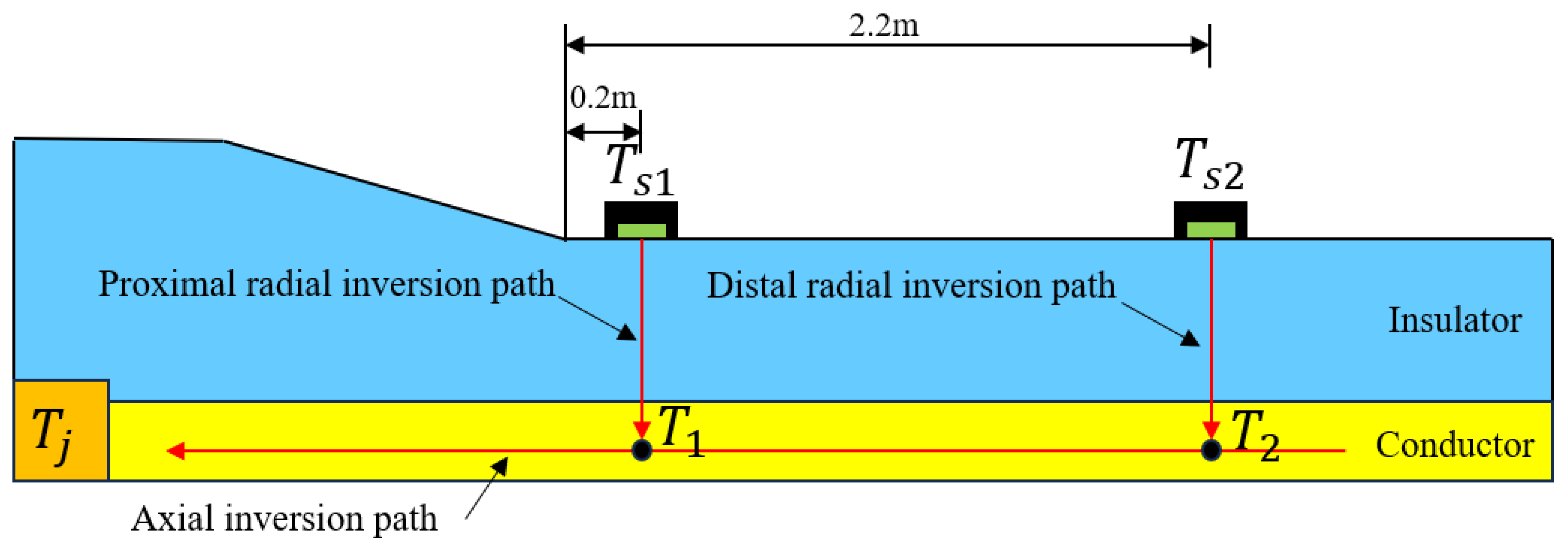
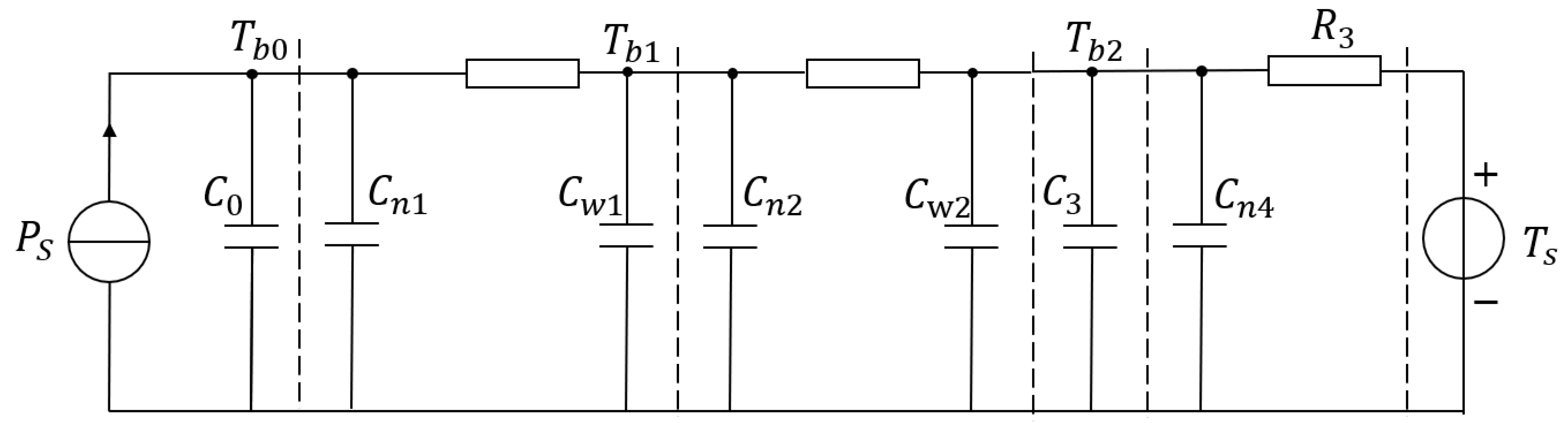
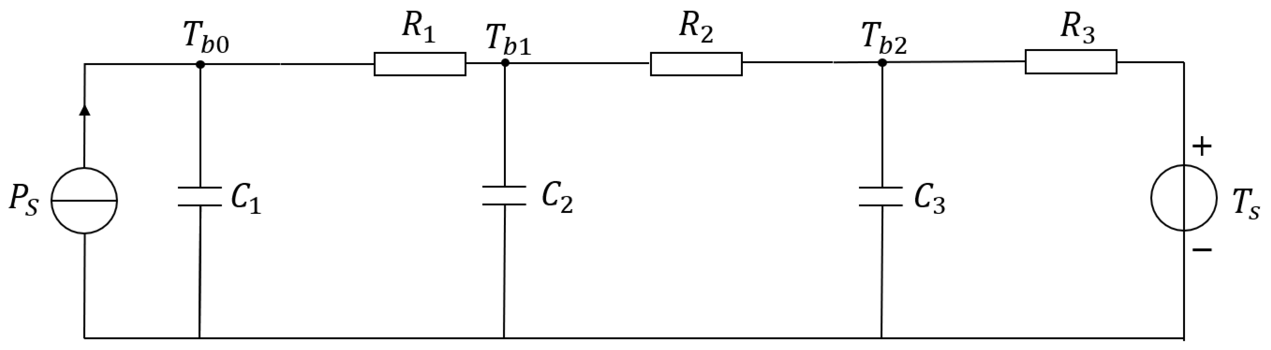
2.1. Radial Inversion Model for the Conductor

Building on the foundation laid by the inversion model for hotspot temperature, we now delve deeper into the specifics of the radial inversion model for the conductor. This model is integral to understanding the thermal dynamics within the cable joint and forms the basis for accurate temperature prediction.

The schematic diagram and parameters of the cable structure are shown in Figure 2. The air layer does not participate in heat transfer and can be omitted in the thermal circuit model. The thermal resistance of the conductor part can be ignored and each remaining layer is equivalently represented as a π-type branch composed of thermal resistance and thermal capacitance.

The value of thermal capacitance is determined by the distribution coefficient p_i:

$$\begin{array}{c}{p}_i=\frac{1}{2ln\left(\frac{r_i}{r_{i-1}}\right)}-\frac{1}{{\left(\frac{r_i}{r_{i-1}}\right)}^2-1}\\ C_{ni}=p_i\cdot C_i\\ C_{wi}=\left(1-p_i\right)\cdot C_i\end{array}$$

(1)

where r_i and r_i−1 are the inner and outer radii of the i-th layer structure. The formulas for calculating the thermal resistance R_i and thermal capacitance C_i of this branch are as follows:

$$\begin{array}{c}{R}_i=\frac{ln\left(\frac{r_i}{r_{i-1}}\right)}{2\pi \lambda }\\ C_i=c_V\pi \left({r_i}^2-{r_{i-1}}^2\right)\end{array}$$

(2)

In the formula, λ is the thermal conductivity of the material and c_V is the volumetric specific heat capacity of the material. Based on the structure of each layer of the cable, a π-type thermal circuit model is obtained, as shown in Figure 3.

By further combining the parallel thermal capacitances, a simplified equivalent thermal circuit model can be obtained, as shown in Figure 4.

Based on the geometric and thermodynamic parameters of the cable and Formulas (1) and (2), the thermal resistance and thermal capacitance parameters in the figure can be determined, as summarized in

Table 1. Thermal resistance and thermal capacitance parameters.

Thermal Circuit Parameters	R1 (K/W)	R2 (K/W)	R3 (K/W)	C1 (J/W)	C2 (J/W)	C3 (J/W)
Values	0.0397	0.0732	0.0478	2876	1567	2312

.

To solve the above transient thermal circuit model, the load current is approximated as a combination of a series of continuous single-step currents and the temperature of each node in each time period is calculated to obtain the temperature change over the entire period. The essence of the above problem is to solve the single-step transient response of the thermal circuit model.

In addressing the transient thermal circuit model, it is essential to accurately capture the temperature dynamics within the cable joint. To achieve this, we approximate the load current as a series of continuous single-step currents, allowing for the calculation of the temperature at each node over time. This approach facilitates the determination of temperature changes throughout the period, essentially solving the single-step transient response of the thermal circuit model.

Two primary methods are employed to solve this model, as follows:

Exact Analytical Solution: This approach utilizes mathematical techniques such as the Laplace transform method and state variable analysis to obtain precise solutions. These methods are particularly suited for systems where exact solutions are achievable and necessary for rigorous analysis.

Approximate Numerical Solution: In contrast, this method simplifies the differential equations into difference equations, significantly enhancing computational efficiency. However, this approximation introduces errors, which are dependent on the time step size. For instance, with time steps of 1 min, 5 min, and 10 min, the maximum errors observed are 0.12 K, 0.52 K, and 0.9 K, respectively. Notably, these errors primarily occur during current steps, while the steady-state error remains negligible. Given these characteristics, the difference equation approach is deemed feasible for the real-time online monitoring of conductor temperature.

The selection between these methods depends on the specific requirements of the thermal model, including the need for accuracy and computational efficiency. By carefully selecting and applying these solution techniques, we can ensure reliable predictions of temperature changes within the cable joint, which is a critical aspect of assessing its thermal performance and overall safety. The solution method of the difference equation for the thermal circuit model is as follows:

Firstly, based on Kirchhoff’s Current Law (KCL), equations are written for Figure 4 and are organized as follows:

$$\left[\begin{array}{c}\frac{d{T}_{b0}}{dt}\\ \frac{d{T}_{b1}}{dt}\\ \frac{d{T}_{b2}}{dt}\end{array}\right]=\left[\begin{array}{ccc}\frac{-1}{R_1{C}_1}& \frac{1}{R_1{C}_1}& 0\\ \frac{1}{R_1{C}_2}& \frac{-\left(R_1+R_2\right)}{R_1{R}_2{C}_2}& \frac{1}{R_2{C}_2}\\ 0& \frac{1}{R_2{C}_3}& \frac{-\left(R_2+R_3\right)}{R_2{R}_3{C}_3}\end{array}\right]\left[\begin{array}{c}{T}_{b0}\\ T_{b1}\\ T_{b2}\end{array}\right]+\left[\begin{array}{cc}\frac{1}{C_1}& 0\\ 0& 0\\ 0& \frac{1}{R_3{C}_3}\end{array}\right]\left[\begin{array}{c}{P}_s\\ T_s\end{array}\right]$$

(3)

In the equation, the heat source P_s(t) can be calculated using the following expression:

$$P_s\left(t\right)=I^2\left(t\right)R$$

(4)

In the equation, R represents the resistance per unit length of the conductor and Equation (3) can be written in the general form of a state equation:

$$\dot{{\rm T}}=A{\rm T}+{\rm B}U$$

(5)

In Equation (5), T(t) is a 3-dimensional state vector, which corresponds to the temperatures at various nodes of the body in the thermal circuit model; $\dot{{\rm T}}$ is the derivative of T(t) with respect to time; A and B are both matrices of real constant coefficients; and U is the input column vector.

By approximating the derivative in Formula (5) as a difference, we can obtain Equation (6):

$$\frac{{\rm T}\left(i+1\right)-{\rm T}\left(i\right)}{\Delta t}=A{\rm T}\left(i+1\right)+{\rm B}U$$

(6)

By organizing Formula (6), we can obtain Equation (7):

$${\rm T}\left(i+1\right)={\left(E-\Delta tA\right)}^{-1}\left({\rm T}\left(i\right)+\Delta t{\rm B}U\right)$$

(7)

In Equation (7), E represents the identity matrix.

To validate the theoretical feasibility of the difference equation method, we employed a transient temperature field simulation designed to mimic a temperature rise test. In this simulation, the initial temperature was set at 25 °C and a current of 1250 A was applied to the cable. The surface temperature of the cable body, taken as input with a time step of 1 min, served as the basis for calculating the conductor temperature using the thermal circuit model. This calculated temperature was then compared with the results from the simulation to assess the accuracy of the model. As illustrated in Figure 5, there is a remarkable agreement between the calculated temperatures and the simulation results, demonstrating the reliability of the difference equation method in predicting conductor temperatures under dynamic conditions. This validation provides confidence in the applicability of the method for real-time online monitoring and reinforces the integrity of our thermal circuit model in capturing the essential thermal behavior of the cable joint.

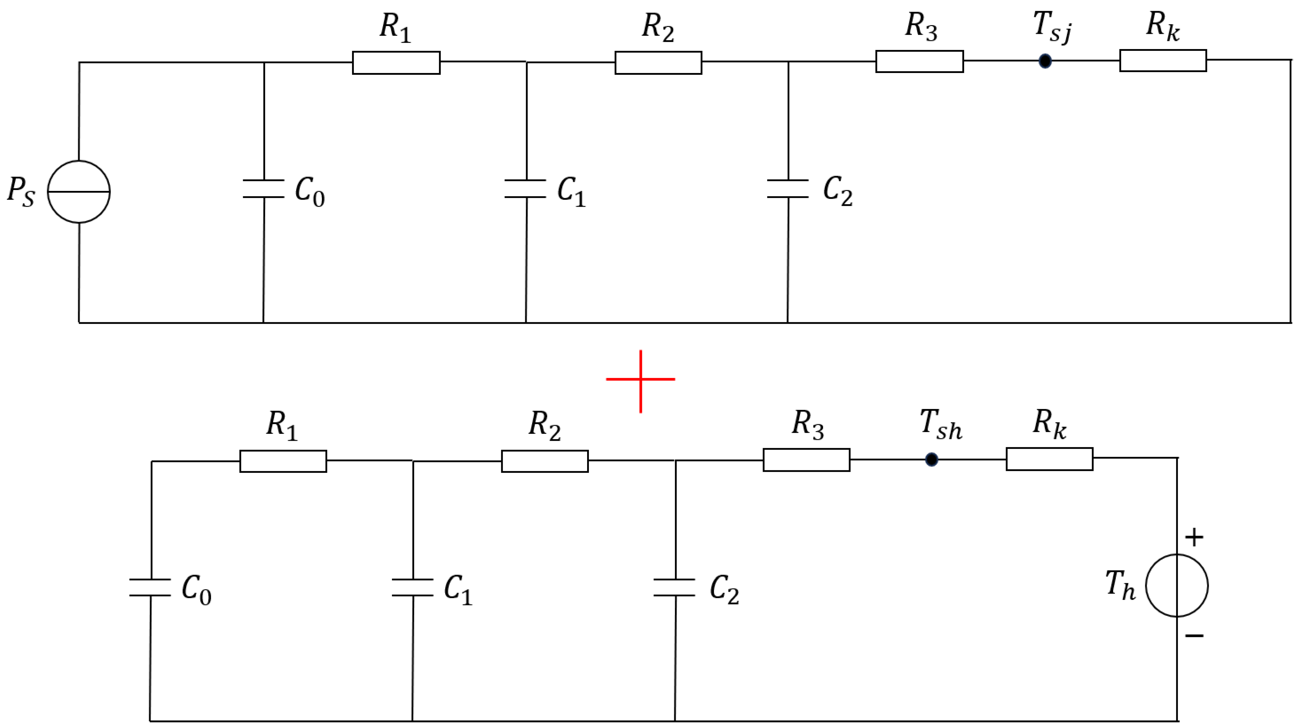
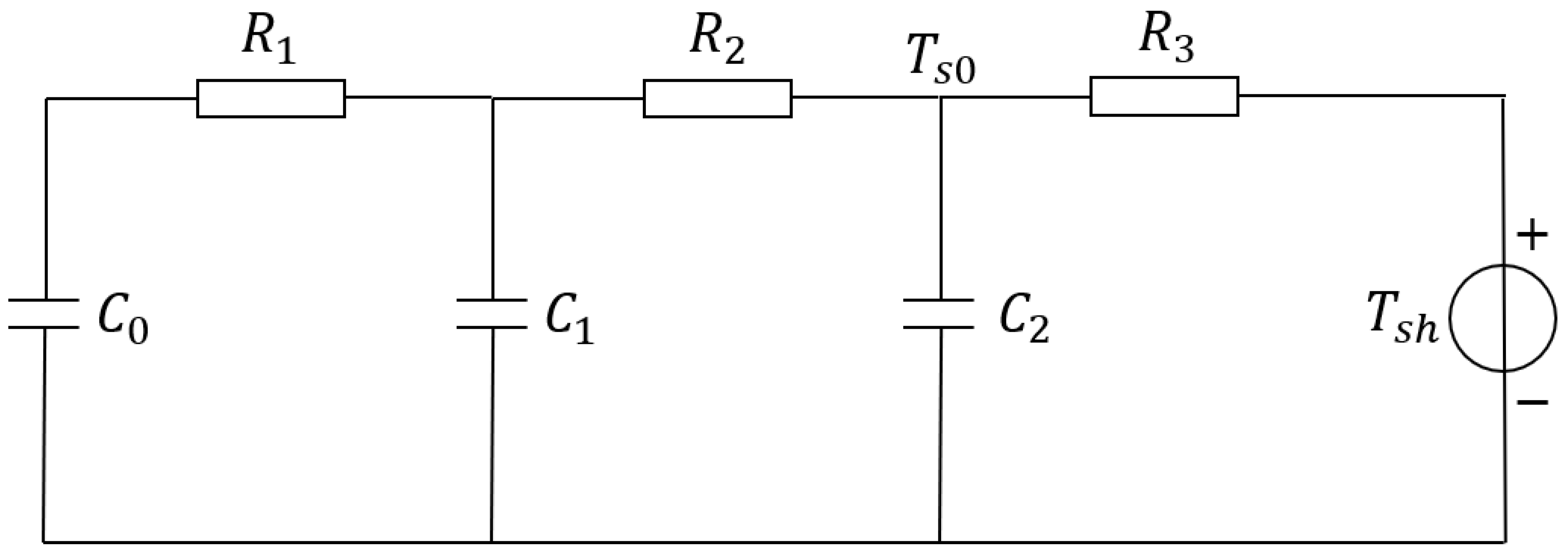
2.2. Conductor Axial Inversion Model

Building on the radial inversion model, we further explore the axial inversion model for the conductor. This model is essential due to the significant structural differences between the shielding cylinder joint and the main body, which prevent the adoption of a unified axial inversion function. Instead, we utilize the equivalent thermal resistance, R_j, of the joint to correct the axial inversion coefficient, a₁, ensuring an accurate representation of the joint’s thermal behavior.

The process begins by calculating the temperature field distribution of the insulated tube mother joint under the condition of contact resistance coefficient k = 1. This step is crucial for understanding the thermal dynamics within the joint. Next, we use Formula (8) to calculate the corresponding equivalent thermal resistance, R_j, of the joint. This value is instrumental in adjusting the axial inversion coefficient, a₁, to account for the joint’s unique thermal characteristics.

With R_j determined, we extract the hotspot temperature, T₀, and the characteristic point temperatures T₁ and T₂. These temperatures are key to assessing the thermal performance of the joint and identifying potential hotspots that could lead to failures. By accurately modeling the axial temperature distribution, we can enhance the reliability and safety of cable intermediate joints in power systems.

$$R_j=\frac{{\stackrel{-}{T}}_{\mathrm{jf}}-{\stackrel{-}{T}}_{\infty }}{{\stackrel{-}{I}}^{2}R}$$

(8)

Importing T₁ and T₂ into the Matlab fitting algorithm, using the following equation for fitting, can be used to determine the axial inversion coefficient a₁:

$$T_j=a_1{T}_1-\left(a_1-1\right)T_2$$

(9)

Set k to 9, 18, 27, and 36, respectively, repeat the above steps, and obtain R_j and a₁ under different contact resistances. Substitute the above data into Formula (9) to fit the function and determine the functional relationship between R_j and a₁ as follows:

$$a_1=4.93-0.69{R_j}^{-2.91}$$

(10)

The axial inversion coefficient a₁ and the heat flow correction coefficient m both depend on R_j, and R_j, in turn, affects a₁ and m, requiring iteration.

3. Dynamic Current Carrying Capacity Assessment

3.1. Calculation of Equivalent Ambient Temperature T_h

In assessing the dynamic current carrying capacity of the cable, a crucial step is determining the equivalent ambient temperature, T_h. This temperature is derived from the surface temperature, T_s, of the cable body using a thermal circuit model. The model is divided into the following two parts: one influenced by the conductor’s Joule heat (T_sj) and the other by environmental excitation (T_sh), as illustrated in Figure 6. The sum of T_sj and Tsh should equal the measured surface temperature, T_sc.

To calculate T_sj, we use the known parameters of the thermal circuit under Joule heat excitation. Then, we derive T_sh as T_sc − T_sj. Applying the substitution theorem, we can treat the air part of the thermal circuit beyond T_sh as a thermal pressure source, as depicted in Figure 7. This allows us to determine the node temperature, T_s0, between resistances R₂ and R₃. Finally, we use the following formula to calculate the equivalent ambient temperature, T_h:

$$T_h=T_{\mathrm{sh}}+\left(T_{\mathrm{sh}}-T_{s0}\right)R_k/R_3$$

(11)

After obtaining the equivalent ambient temperature T_h, the environmental heating temperature, T_j2, at the corresponding moment can be calculated using the following formula:

$$T_{j2}\left(t\right)=T_h\left(t\right)+\left(T_{j2}\left(t-\Delta t_d\right)-T_h\left(t\right)\right)\mathit{exp}\left(-\Delta t_d/{\tau }_{j2}\right)$$

(12)

3.2. Calculation of Environmental Heating Temperature T_j2

In assessing the dynamic current carrying capacity of cables, an important step is the prediction of the environmental heating temperature, T_j2. For this purpose, we employ the Prophet model, which excels at decomposing time series data into seasonal, trend, holiday, and residual components [19,20,21]. This decomposition allows for separate forecasting of each type of data, with the final prediction result obtained by their superposition.

The core of the Prophet model is an additive model, represented by the following formula [22,23,24,25,26,27]:

$$y\left(t\right)=g\left(t\right)+s\left(t\right)+h\left(t\right)+\epsilon \left(t\right)$$

(13)

In the context of dynamic current carrying capacity prediction, it is essential to consider the periodicity of cable load and environmental factors. The trend component g(t) of load and environmental changes plays a pivotal role in this analysis. According to practical engineering experience, the most significant trend within this component is a non-periodic change trend of data.

Specifically, when focusing solely on environmental factors, the trend component can be divided into two parts based on time constants. The small time constant part represents the daily environmental temperature trend, capturing the temperature fluctuations within a 24 h Earth cycle. Conversely, the large time constant part encapsulates the annual environmental temperature trend, reflecting the temperature variations within a 365 day solar cycle. Understanding these trends is crucial for accurately predicting the dynamic current carrying capacity of cables, as it allows for a comprehensive analysis of both short-term and long-term environmental impacts. The model for processing environmental temperature trend components is selected as follows:

In time series forecasting, the logistic growth model is generally used to organize the trend component. The logistic growth model is g(t):

$$g\left(t\right)=\frac{C\left(t\right)}{1+e^{\left(-k\left(t-b\left(t\right)\right)\right)}}$$

(14)

Here, k is the growth rate; b(t) is the offset; C(t) is the capacity of the model; and as t increases, g(t) approaches C(t) gradually.

Here, we first discuss the improvement of the logistic growth model. The traditional logistic growth model predicts a time trend described by k and b. Based on the above expression, for the prediction of the long-term dynamic load capacity of cables, there should be two trend components, as follows: one for the daily environmental temperature change and one for the annual environmental temperature change. Therefore, the above model is improved as follows:

$$g\left(t\right)=\frac{C\left(t\right)}{1+e^{\left(-k1\left(t-b1\left(t\right)\right)\right)}+e^{\left(-k2\left(t-b2\left(t\right)\right)\right)}}$$

(15)

where k₁ and b₁ describe the daily temperature change trend and k₂ and b₂ describe the annual environmental temperature change trend (the physical meaning of these two parameters is discussed later). C(t) is the capacity of the model.

Now, physical meanings are assigned to k₁, b₁, k₂, b₂, and C(t).

Since k₁ and b₁ describe the daily temperature change trend and k₂ and b₂ describe the annual environmental temperature change trend, the trend component e^{(−k1(t − b1(t)))} is fitted with the daily temperature change; that is, y = e^{(−k1(t − b1(t)))}, where y is the temperature and t is the time.

To fit and predict seasonal effects, Prophet proposes a flexible model based on Fourier series, and s(t) can be estimated using the following formula. The reason for choosing this model is the periodicity in the cable dynamic current carrying capacity system, which is reflected in the periodicity of daily variables. Based on life experience, it is not difficult to conclude that within a certain number of days, for a specific cable line, the measured temperature shows a periodic change with a period of 24 h. Of course, there may be a bias due to the overall temperature rise or fall, but when this bias is not considered, the environmental temperature shows periodicity. Once the periodicity is considered for fitting, trigonometric functions are considered at first, so this paper only introduces simple trigonometric functions as the periodic component.

$$s\left(t\right)=a_n\cos \left(\frac{2\pi nt}{T}\right)$$

(16)

T is a fixed period, here taken as the period of annual data, which is 365; 2n is the number of times used in the model, here chosen as 2n = 1.

For the prediction of the environmental temperature of a cable:

$$Y\left(t\right)=g\left(t\right)+s\left(t\right)$$

(17)

Since the load change pattern of each cable is different, this invention extracts the daily load peaks of each cable that needs dynamic current carrying capacity in recent years to establish a Prophet time series load model. The input data of the Prophet time series load model for cables are the time, t_s, and the corresponding environmental temperature, l, at that time, as shown in the following formula:

$$s=\left[t_1,t_2,\dots .t_n\right]$$

(18)

$$l=\left[l_1,l_2,\dots .l_n\right]$$

(19)

The trained PROPHET model is used to predict the test samples, and the results are shown in Figure 8. The predicted values follow the experimental values well, with a maximum error of less than 5 K and an average absolute error of less than 0.6 K, indicating good performance.

To validate the practicality of the proposed dynamic current carrying capacity prediction model, this study conducted comprehensive temperature rise tests on a meticulously designed experimental platform. It is crucial to emphasize that dynamic augmentation operations are only applicable for cable joints with normal contact resistance. For joints exhibiting poor contact, there is an inherent safety hazard even under rated current operation, rendering augmentation operations inadvisable. Consequently, the dynamic current carrying capacity test in this study is exclusively conducted on joints with satisfactory contact status. In the detailed procedure of the dynamic current carrying capacity test, the rated current is initially passed through the insulated cable to simulate the load condition of the actual equipment prior to dynamic augmentation. This step is essential to ensure that the conditions closely resemble real-world scenarios. If the hotspot temperature of the joint consistently remains lower than and close to the temperature limit of 90 °C, the dynamic current carrying capacity prediction model can be deemed effective. Conversely, if the hotspot temperature exceeds this limit, the prediction is considered unsuccessful. The experimental setup is shown in Figure 9, where four intermediate joints are set with different sampling resistances at the preset stage. This schematic illustrates an experimental setup designed to dynamically predict the current carrying capacity of cable joints by adjusting the current with a voltage regulator. Current measurements are monitored by an ammeter (denoted as ‘I’) and temperature readings are taken at various points (denoted as T1, T2, T3, and T4) along the cable. Surface temperatures are measured using an optical surface temperature measurement device (denoted as T_s). This method combines surface temperature readings with an algorithm to predict the dynamic load capacity of the cables.

Additionally, the setup features four intermediate joints preset with different sampling resistances to simulate varying resistance conditions found in actual cable systems. These sampling resistances allow for a more nuanced examination of the cable’s behavior under different electrical loads. By comparing the algorithm’s predictions with the actual temperatures measured at the internal temperature measurement points (T_s1, T_s2), the effectiveness of the predictive method can be validated, ensuring that the model’s forecasts are accurate reflections of the cable’s performance in real-world conditions. The actual object is shown in Figure 10.

In the initial phase of the experiment, the temperature limit, Tm, of the prediction formula was set at 90 °C to align with typical industry standards. Two separate tests were conducted to validate the model’s reliability and repeatability. Both tests commenced augmentation at approximately 8 a.m., with the rated current passing through the cable to achieve a steady state before augmentation, as depicted in Figure 11. The first test concluded at around 6 p.m., while the second test extended until midnight, providing a comprehensive assessment over a full day cycle.

Selection of Hyperparameters

Thermal Circuit Parameters: The thermal resistance (R) and thermal capacitance (C) parameters are crucial for accurately modeling the thermal behavior of the cable joint. These parameters are determined based on the geometric and thermodynamic properties of the cable, as summarized in Table 1 of this article. The selection of these parameters is essential for capturing the heat transfer dynamics within the cable joint.

Time Step Size for Numerical Solution: This article mentions that the approximate numerical solution method introduces errors dependent on the time step size. For example, time steps of 1 min, 5 min, and 10 min result in different errors. Selecting an appropriate time step size is crucial for balancing computational efficiency with the accuracy of the thermal circuit model.

Axial Inversion Coefficient (a₁): The axial inversion model for the conductor is used to assess the thermal performance of the cable joint and identify potential hotspots. The axial inversion coefficient (a₁) is adjusted based on the equivalent thermal resistance (R_j) of the joint, to ensure an accurate representation of the joint’s thermal behavior. This article describes a process for calculating R_j and a₁ and for fitting their functional relationship.

Heat Flow Correction Coefficient (m): The dynamic current carrying capacity assessment involves calculating the equivalent ambient temperature (T_h) using a thermal circuit model. The heat flow correction coefficient (m) is used in conjunction with the axial inversion coefficient (a₁) to accurately model the thermal response of the cable joint to both conductor Joule heat and environmental excitation.

The test results are enlightening, revealing that in the initial stage of dynamic augmentation, the dynamic current carrying capacity reaches its peak, surpassing the rated current by 60%. This is attributed to the conductor temperature under the rated current being significantly lower than the temperature limit, indicating substantial potential for dynamic augmentation. As the test progresses, the current carrying capacity gradually decreases, dynamically adjusting in response to environmental changes. This dynamic adaptation is a critical feature of the model, enabling it to cater to varying load demands and environmental conditions.

Furthermore, the dynamic augmentation multiple varies approximately between 10% and 50%, depending on the time of day and environmental factors. This variability underscores the model’s sensitivity to external conditions and its ability to optimize current carrying capacity accordingly. The tests conducted in this study provide valuable insights into the model’s performance and its potential applications in enhancing the efficiency and safety of electrical power systems.

The current carrying capacity is lower during the day and higher at night, with the dynamic augmentation multiple varying between 10% and 50%. Since the experiment was conducted in the summer, it can be expected that the dynamic current carrying capacity of the joint will increase significantly in the winter. During the experiment, the conductor temperature fluctuated around 85 °C and the highest hotspot temperature in the tests was slightly above the temperature limit, reaching 85.58 °C, which may accelerate the aging of the insulation material. Ideally, dynamic augmentation should keep the conductor temperature stably below and quite close to 85 °C, but there will inevitably be some deviation in actual application. The corresponding error is shown in Figure 12 and, as shown in Figure 12, the control error continues to be under 5 K after 12:00.

To elaborate further, within the same control strategy, the temperature and load curve of another contact point, which has a lower contact resistance, is shown in Figure 13. It can be observed that the load curves of the two are the same. However, due to the lower contact resistance of the other joint, its hotspot temperature is generally lower than that of the first joint, yet it follows the same trend with the changes in load.

An analysis of Figure 11 and Figure 13 reveals that under the current carrying capacity control based on the joint depicted in Figure 11, another joint on the same line demonstrates a similar trend in hotspot temperature changes. Due to this joint having lower electrical resistance, its overall temperature is also lower. As direct measurement of contact resistance is challenging, resistance values are not provided here. Moreover, the temperature at the hotspot of Joint 2 correlates with the current variation trend consistent with Joint 1. However, due to hardware issues with the measurement equipment, some data were lost. The approach taken in the figure is to omit the missing data and connect the remaining valid data points, which results in some apparent discontinuities. Nonetheless, this does not affect the conclusion of the paper. It serves as a sort of indirect proof, further illustrating the effectiveness of the method.

4. Conclusions

This paper takes the 110 kV cable middle joint as its research object, constructs the path of radial inversion of the body and axial inversion of the conductor with heat flow as the bridge, and performs a real-time inversion of the conductor temperature. Based on the above inversion results, combined with the temperature measurement information on the cable surface, the environmental change is predicted using the PROPHET time series model analysis method and a dynamic current carrying capacity assessment method for the cable middle joint is proposed. Finally, a dynamic current carrying capacity test is designed and conducted to improve and verify the prediction algorithm. The main research conclusions are as follows:

(1) The combination inversion of the hotspot temperature using the surface temperature at the characteristic points is in good agreement with the actual measurement values. Under different environmental conditions and current loading methods, the inversion error does not exceed 10 K.

(2) A dynamic current carrying capacity rolling prediction method for the insulated tube mother joint is proposed, whereby the temperature field of the joint is equivalent to the superposition of two first-order thermal circuits, and the excitations of the two thermal circuit models are, respectively the conductor Joule heat source and the equivalent ambient temperature. The responses generated by the above excitations at the hotspot of the joint are the conductor heating temperature rise and the environmental heating temperature, respectively. The PROPHET time series prediction model is constructed using historical data for rolling prediction. The test results show that the prediction accuracy of the environmental temperature in dynamic current carrying prediction is high.

References

1. Lü, G.M.; Zhang, D.L.; Fu, C.W.; Yang, L.M.; Zhou, C.C.; Wu, X.J.; Liu, B.D. Development and testing of XLPE cables and accessories with temperature measuring optical fibers embedded in segmented conductors. Wire Cable 2013, 5, 8–14. [Google Scholar]
2. Qiu, W.H.; Yang, L.; Hao, Y.P.; Chen, Y.; Deng, S.H.; Wen, Z.M. Temperature monitoring experiment of XLPE cables with embedded distributed optical fibers. Guangdong Electr. Power 2018, 8, 175–181. [Google Scholar]
3. Nakamura, S.; Morooka, S.; Kawasaki, K. Conductor temperature monitoring system in underground power transmission XLPE cable joints. IEEE Trans. Power Deliv. 1992, 7, 1688–1697. [Google Scholar] [CrossRef]
4. Tong, Z.J.; Zhou, N.R.; Duan, Q.S.; He, C.; Wang, Y.C.; Jin, X.T. Study on conductor temperature detection of T-type cable joints in ring main units based on thermal circuit method. Sens. Microsyst. 2017, 11, 131–138. [Google Scholar]
5. Pilgrim, J.A.; Swaffield, D.J.; Lewin, P.L.; Larsen, S.T.; Payne, D. Assessment of the impact of joint bays on the ampacity of high-voltage cable circuits. IEEE Trans. Power Deliv. 2009, 24, 1029–1036. [Google Scholar] [CrossRef]
6. Chang, W.Z.; Han, X.H.; Li, C.R.; Ge, Z.D. Experimental study on temperature measurement technology of cable middle joints under step current. High Volt. Eng. 2013, 39, 1156–1162. [Google Scholar]
7. Yang, F.; Cheng, P.; Luo, H.; Yang, Y.; Liu, H.; Kang, K. 3-D thermal analysis and contact resistance evaluation of power cable joint. Appl. Therm. Eng. 2016, 93, 1183–1192. [Google Scholar] [CrossRef]
8. Yang, F.; Liu, K.; Cheng, P.; Wang, S.; Wang, X.; Gao, B.; Fang, Y.; Xia, R.; Ullah, I. The coupling fields characteristics of cable joints and application in the evaluation of crimping process defects. Energies 2019, 9, 932. [Google Scholar] [CrossRef]
9. Liu, G.; Wang, Z.H.; Xu, T.; Liu, Y.G.; Wang, P.Y. Calculation and experimental analysis of current carrying capacity of 110 kV cable middle joints. High Volt. Eng. 2017, 43, 1670–1676. [Google Scholar]
10. Wang, P.; Liu, G.; Ma, H.; Liu, Y.; Xu, T. Investigation of the ampacity of a prefabricated straight-through joint of high voltage cable. Energies 2017, 10, 1–17. [Google Scholar] [CrossRef]
11. Liu, G.; Wang, P.Y.; Mao, J.K.; Liu, L.F.; Liu, Y.G. Simulation calculation of temperature field distribution of high voltage cable joints. High Volt. Eng. 2018, 44, 3688–3698. [Google Scholar]
12. Liu, G.; Wang, P.Y.; Wang, Z.H.; Xu, T.; Liu, Y.G.; Han, Z.Z. Method for determining the current carrying capacity of high voltage AC cable joints based on ANSYS. J. South China Univ. Technol. (Nat. Sci. Ed.) 2017, 4, 22–29. [Google Scholar]
13. Dai, Y.; Cheng, Y.C.; Zhong, W.L.; Lin, J.D. Dynamic Capacity Enhancement Technology for High Voltage Overhead Transmission Lines; China Electric Power Press: Beijing, China, 2013. [Google Scholar]
14. Patton, R.N.; Kim, S.K.; Podmore, R. Monitoring and rating of underground power cables. IEEE Trans. Power Appar. Syst. 1979, 98, 2285–2293. [Google Scholar] [CrossRef]
15. Ren, L.J.; Jiang, X.C.; Sheng, G.H.; Sun, X.M. Chaotic prediction of the allowable transmission capacity of transmission lines. Proc. CSEE 2009, 29, 86–91. [Google Scholar]
16. Ren, L.J. Technology for Dynamically Increasing the Transmission Capacity of Transmission Lines Based on Conductor Tension. Ph.D. Dissertation, Shanghai Jiao Tong University, Shanghai, China, 2008. [Google Scholar]
17. Shang, Z.; Hossain, M.; Wycisk, R.; Pintauro, P.N. Poly(phenylene sulfonic acid)-expanded polytetrafluoroethylene composite membrane for low relative humidity operation in hydrogen fuel cells. J. Power Sources 2022, 535, 231375. [Google Scholar] [CrossRef]
18. Mondal, A.N.; Wycisk, R.; Waugh, J.; Pintauro, P.N. Electrospun Si and Si/C Fiber Anodes for Li-Ion Batteries. Batteries 2023, 9, 569. [Google Scholar] [CrossRef]
19. Tang, L.Z. Study on Hotspot Temperature Inversion and Dynamic Ampacity Forecasting for Insulated Busbar Joints. Ph.D. Thesis, Wuhan University, Wuhan, China, 2020. [Google Scholar]
20. Toharudin, T.; Pontoh, R.S.; Caraka, R.E.; Chen, R.C. Employing Long Short-Term Memory and Facebook Prophet Model in Air Temperature Forecasting. Commun. Stat.-Simul. Comput. 2021, 52, 279–290. [Google Scholar] [CrossRef]
21. Arai, K.; Fujikawa, I.; Nakagawa, Y.; Momozaki, T.; Ogawa, S. Modified Prophet+Optuna Prediction Method for Sales Estimations. Int. J. Adv. Comput. Sci. Appl. 2022, 13, 2022. [Google Scholar] [CrossRef]
22. Ji, J.; Zhang, J.; Liu, L. Forecasting container freight rates using the Prophet forecasting method. Transp. Res. Part E Logist. Transp. Rev. 2021, 154, 102390. [Google Scholar]
23. Angelopoulos, S.; Siskos, K.; Psarras, J.; Hong, T.; Liu, H. A hybrid forecasting model using LSTM and Prophet for energy consumption prediction. Energy Rep. 2020, 6, 291–299. [Google Scholar]
24. Krajewski, W.F.; Mantilla, R.; Quintero, F. Evaluation of random forests and Prophet for daily streamflow forecasting. Adv. Geosci. 2018, 45, 201–208. [Google Scholar]
25. Lee, Y.; Son, Y. Prediction of global omicron pandemic using ARIMA, MLR, and Prophet methods. Sci. Rep. 2022, 12, 2904. [Google Scholar]
26. Solomatine, D.P.; Ostfeld, A. Data-driven modelling: Some past experiences and new approaches. J. Hydroinformatics 2008, 10, 3–22. [Google Scholar] [CrossRef]
27. Jordan, A.; Krüger, F.; Lerch, S. Evaluating probabilistic forecasts with the R package scoring Rules. arXiv 2018, arXiv:1709.04743. [Google Scholar]
Figure 1. Inversion path of hotspot temperature at joints.
Processes 12 00748 g001
Figure 2. The structure of the cable. 1—cable core; 2—inner shielding layer; 3—XLPE; 4—outer shielding layer; 5—semi-conductive water-blocking tape; 6—corrugated aluminum sheath; 7—outer sheath.
Processes 12 00748 g002
Figure 3. π-type thermal circuit model.
Processes 12 00748 g003
Figure 4. A simplified equivalent thermal circuit model.
Processes 12 00748 g004
Figure 5. Accuracy of radial temperature inversion of cable body.
Processes 12 00748 g005
Figure 6. Decomposition of the equivalent thermal circuit model of the cable body.
Processes 12 00748 g006
Figure 7. Application of the substitution theorem to the thermal circuit model.
Processes 12 00748 g007
Figure 8. Environmental heating temperature prediction.
Processes 12 00748 g008
Figure 9. Experimental setup.
Processes 12 00748 g009
Figure 10. Experimental setup picture.
Processes 12 00748 g010
Figure 11. Dynamic current carrying capacity test for cables.
Processes 12 00748 g011
Figure 12. Corresponding error.
Processes 12 00748 g012
Figure 13. Temperature of another joint with lower resistance.
Processes 12 00748 g013