
Reliability-Based Preventive Maintenance Strategy for Subsea Control System
Abstract
:1. Introduction
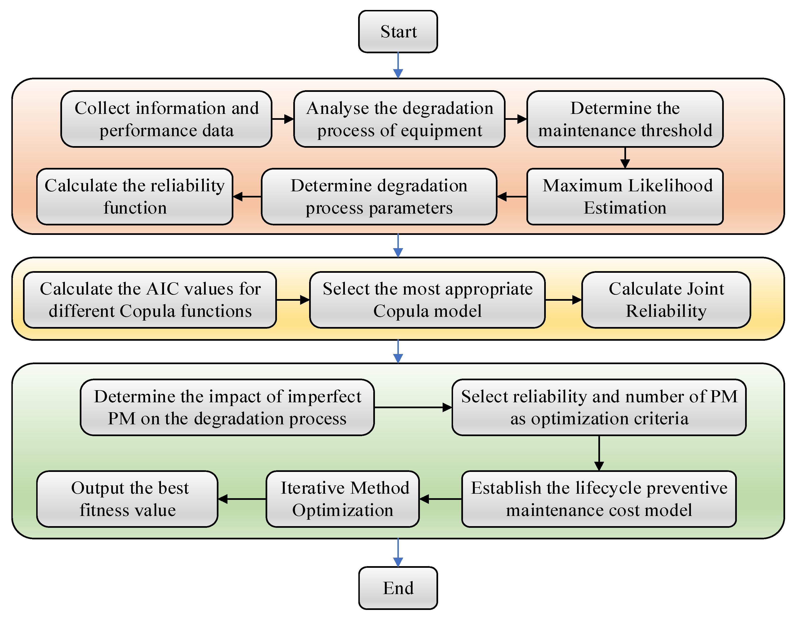
2. Methodology
2.1. Definition and Properties of Wiener Process
- ;
- For any , random variables, and the increments , …, are mutually independent random variables;
- For any , , , where is the drift coefficient and is the diffusion coefficient.
2.2. Parameter Estimation of the Wiener Process
2.3. Reliability Modeling Method Based on Wiener Process
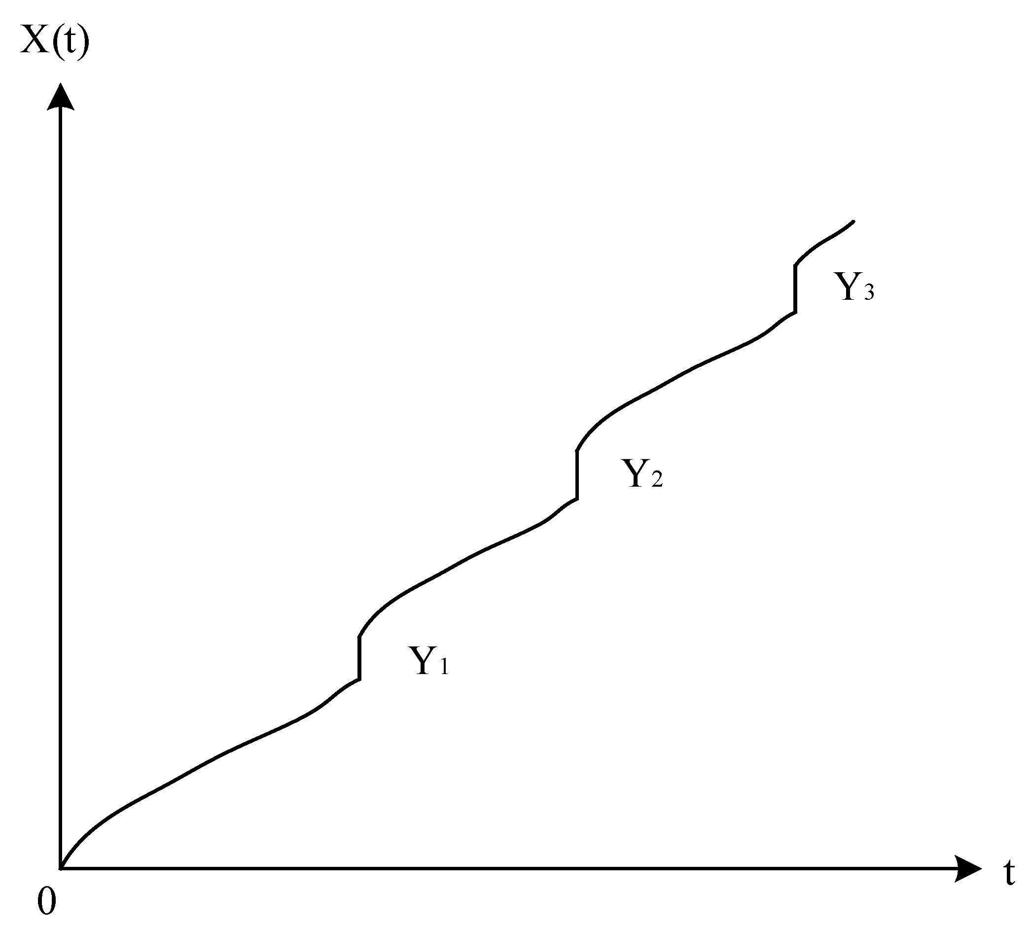
2.4. Reliability Modeling Method Considering the Impact of Random Shocks
3. Modeling
- The Wiener process, preferred over the Weibull and Gamma distributions for its accuracy in representing the natural degradation of electronic components, is adopted due to its compatibility with the redundancy and complex coupling in subsea control systems. It aligns more closely with observed reliability trends.
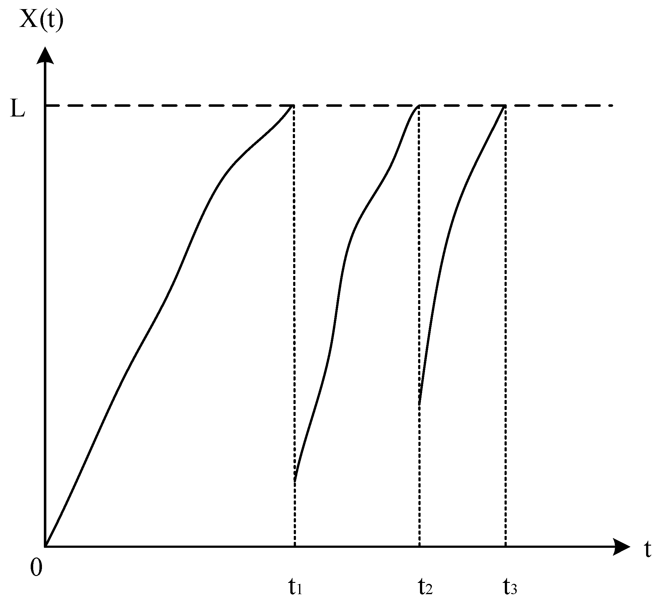
- It is presumed that all components are new at commissioning and receive timely maintenance to avert potential operational failures, where “timely” implies immediate action upon detecting degradation or reaching a maintenance interval.
- The model accounts for external shocks such as natural disasters or sudden operational changes, considering their discrete, sudden nature and independence. It aims to quantify their impact in terms of frequency and intensity.
- Replacement is anticipated during the Nth PM cycle, triggered when reliability dips below a pre-determined threshold, which is informed by historical data analysis and equipment performance criteria, to ensure maintenance precedes significant deterioration.
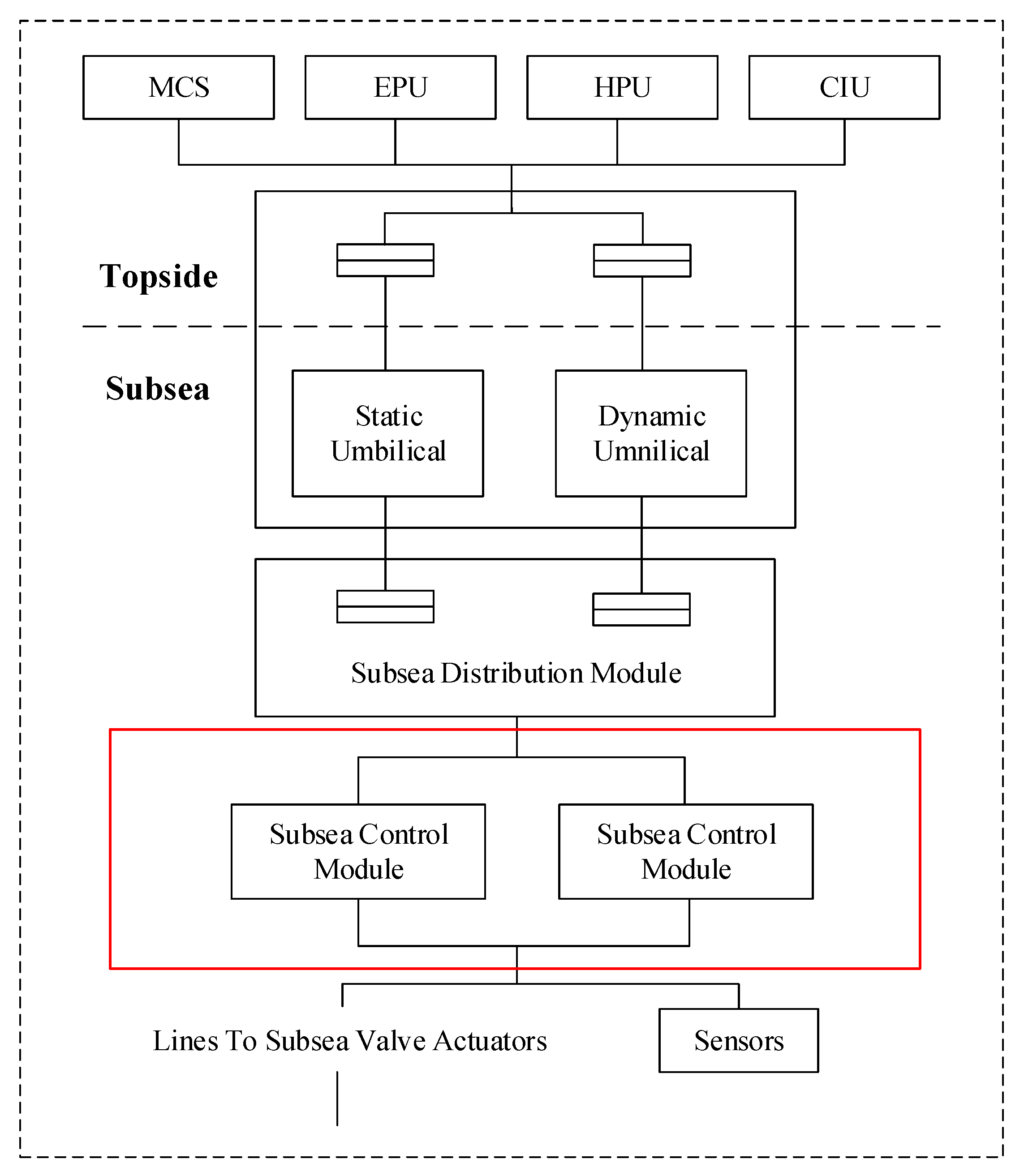
3.1. Redundant System Reliability Modeling
- Clayton Copula;
- Gumbel Copula.
3.2. Imperfect PM Modeling
4. SCM Maintenance Case Simulation
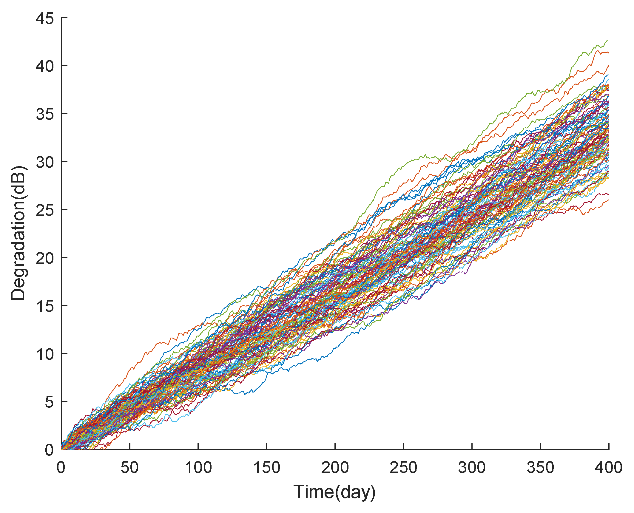
4.1. SCM Performance Degradation Data Simulation
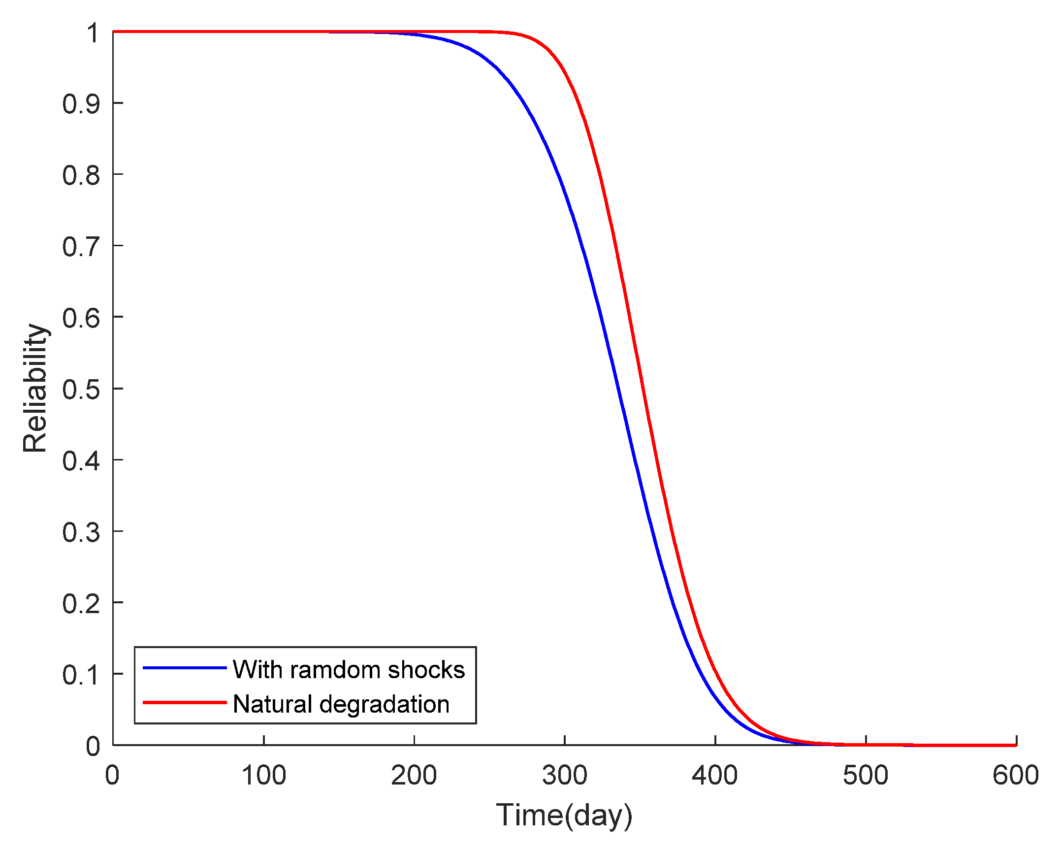
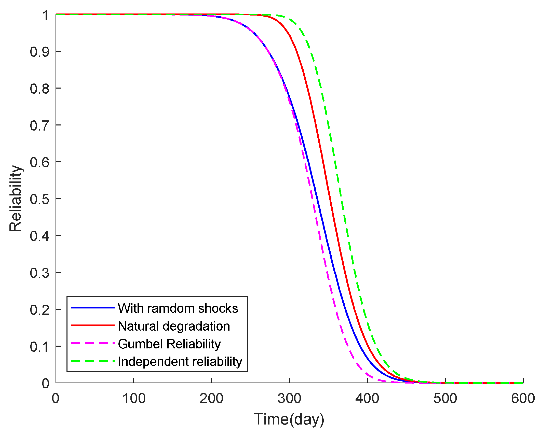
4.2. SCM Reliability Modeling Simulation
4.3. Imperfect PM strategies of SCM
5. Conclusions
Author Contributions
Funding
Data Availability Statement
Conflicts of Interest
References
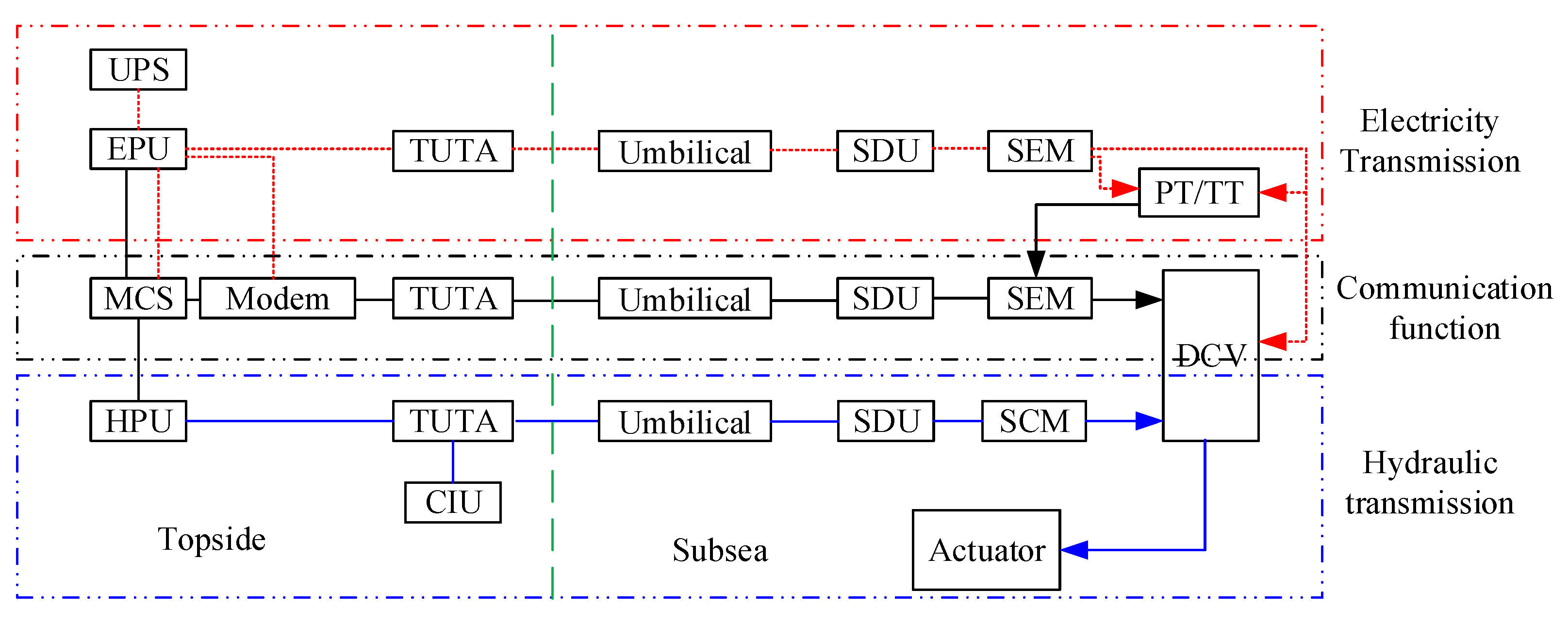
- Yamamoto, M.; Almeida, C.F.; Angelico, B.A.; Colon, D.; Salles, M.B. Integrated subsea production system: An overview on energy distribution and remote control. In Proceedings of the 2014 IEEE Petroleum and Chemical Industry Conference—Brasil (PCIC Brasil), Rio de Janeiro, Brazil, 25–27 August 2014; pp. 173–181. [Google Scholar] [CrossRef]
- Hansen, R.L.; Rickey, W.P. Evolution of subsea production systems: A worldwide overview. J. Pet. Technol. 1995, 47, 675–680. [Google Scholar] [CrossRef]
- Bednar, J.M. Zinc subsea production system: An overview. J. Pet. Technol. 1994, 46, 346–352. [Google Scholar] [CrossRef]
- Sotoodeh, K. A review on subsea process and valve technology. Mar. Syst. Ocean. Technol. 2019, 14, 210–219. [Google Scholar] [CrossRef]
- Lyalla, I.; Arulliah, E.; Innes, D. A critical analysis of open protocol for subsea production controls system communication. In Proceedings of the OCEANS 2017, Aberdeen, UK, 19–22 June 2017; pp. 1–7. [Google Scholar] [CrossRef]
- Zhang, Y.; Tang, W.; Du, J. Development of subsea production system and its control system. In Proceedings of the 2017 4th International Conference on Information, Cybernetics and Computational Social Systems (ICCSS), Dalian, China, 24–26 July 2017; pp. 117–122. [Google Scholar] [CrossRef]
- SINTEF. OREDA Offshore and Onshore Reliability Data Handbook, Vol 1.—Topside Equipment and Vol. 2—Subsea Equipment, 6th ed.; OREDA Participants: Høvik, Norway, 2015. [Google Scholar]
- Zuo, X.; Yu, X.; Yue, Y.; Yin, F.; Zhu, C. Reliability Study of Parameter Uncertainty Based on Time-Varying Failure Rates with an Application to Subsea Oil and Gas Production Emergency Shutdown Systems. Processes 2021, 9, 2214. [Google Scholar] [CrossRef]
- Orošnjak, M.; Brkljač, N.; Šević, D.; Čavić, M.; Oros, D.; Penčić, M. From predictive to energy-based maintenance paradigm: Achieving cleaner production through functional-productiveness. J. Clean. Prod. 2023, 408, 137177. [Google Scholar] [CrossRef]
- Gao, H.; Cui, L.; Qiu, Q. Reliability Modeling for Degradation-Shock Dependence Systems with Multiple Species of Shock. Reliab. Eng. Syst. Saf. 2019, 185, 133–143. [Google Scholar] [CrossRef]
- Liu, W.; Wang, X.; Li, S. Study on the Effect of Failure Threshold Change Rate on Product Reliability Based on Performance Degradation. J. Fail. Anal. Prev. 2020, 20, 448–454. [Google Scholar] [CrossRef]
- Liu, Z.; Liu, Y. A Bayesian network based method for reliability analysis of subsea blowout preventer control system. J. Loss Prev. Process Ind. 2019, 59, 44–53. [Google Scholar] [CrossRef]
- Ali, L.; Jin, S.; Bai, Y. Risk Assessment and reliability analysis of subsea production Systems. In Proceedings of the International Conference on Offshore Mechanics and Arctic Engineering, American Society of Mechanical Engineers, Virtual, 3–7 August 2020. V02AT02A076. [Google Scholar] [CrossRef]
- Si, X.; Wang, W.; Hu, C.; Chen, M.; Zhou, D. A Wiener-process-based degradation model with a recursive filter algorithm for remaining useful life estimation. Mech. Syst. Signal Process. 2013, 35, 219–237. [Google Scholar] [CrossRef]
- Narayanaswamy, V.; Raju, R.; Durairaj, M.; Ananthapadmanabhan, A.; Annamalai, S.; Ramadass, G.A.; Atmanand, M.A. Reliability-centered development of deep water ROV ROSUB 6000. Mar. Technol. Soc. J. 2013, 47, 55–71. [Google Scholar] [CrossRef]
- Liu, Y.; Ma, L.; Sun, L.; Zhang, X.; Yang, Y.; Zhao, Q.; Qu, Z. Risk-Based Maintenance Optimization for a Subsea Production System with Epistemic Uncertainty. Symmetry 2022, 14, 1672. [Google Scholar] [CrossRef]
- Zhou, B.; Shi, Y.; Zhang, Y. Availability-centered Maintenance Policies for Degrading Manufacturing Systems Considering Product Quality. J. Northeast. Univ. (Nat. Sci.) 2021, 42, 814–820. [Google Scholar] [CrossRef]
- Zhen, X.; Hua, Y.; Huang, Y. Optimization of preventive maintenance intervals integrating risk and cost for safety critical barriers on offshore petroleum installations. Process Saf. Environ. Prot. 2021, 152, 230–239. [Google Scholar] [CrossRef]
- Sun, H.; He, D.; Zhong, J. Preventive maintenance optimization for key components of subway train bogie with consideration of failure risk. Eng. Fail. Anal. 2023, 154, 107634. [Google Scholar] [CrossRef]
- Wu, C.; Pan, R.; Zhao, X.; Wang, X. Designing preventive maintenance for multi-state systems with performance sharing. Reliab. Eng. Syst. Saf. 2024, 241, 109661. [Google Scholar] [CrossRef]
- Pereira, F.H.; Melani, A.H.D.A.; Kashiwagi, F.N.; Rosa, T.G.D.; Santos, U.S.D.; Souza, G.F.M.D. Imperfect Preventive Maintenance Optimization with Variable Age Reduction Factor and Independent Intervention Level. Appl. Sci. 2023, 13, 10210. [Google Scholar] [CrossRef]
- Zhao, J.; Gao, C.; Tang, T. A Review of Sustainable Maintenance Strategies for Single Component and Multicomponent Equipment. Sustainability 2022, 14, 2992. [Google Scholar] [CrossRef]
- Barron, Y.; Yechiali, U. Generalized control-limit preventive repair policies for deteriorating cold and warm standby Markovian system. Lise. Trans. 2017, 49, 1031–1049. [Google Scholar] [CrossRef]
- Barron, Y. Group maintenance policies for an R-out-of-N system with phase-type distribution. Ann. Oper. Res. 2018, 261, 79–105. [Google Scholar] [CrossRef]
- Abbou, A. Maintenance Optimization of Partially Observable Complex Systems. Ph.D. Thesis, University of Toronto, Toronto, ON, Canda, 2020. [Google Scholar]
- Liang, Z.; Parlikad, A.K. Predictive group maintenance for multi-system multi-component networks. Reliab. Eng. Syst. Saf. 2020, 195, 106704. [Google Scholar] [CrossRef]
- Agergaard, J.K.; Sigsgaard, K.V.; Mortensen, N.H.; Ge, J.; Hansen, K.B. Quantifying the impact of early-stage maintenance clustering. J. Qual. Maint. Eng. 2023, 29, 1–15. [Google Scholar] [CrossRef]
- Desnica, E.; Ašonja, A.; Radovanović, L.; Palinkaš, I.; Kiss, I. Selection, dimensioning and maintenance of roller bearings. Lect. Notes Netw. Syst. 2022, 592, 133–142. [Google Scholar] [CrossRef]
- Novaković, B.; Desnica, E.; Radovanović, L.J.; Ivetić, R.; Đorđević, L.; Labović Vukić, D. Optimization of industrial fan system using methods laser alignment. Appl. Eng. Lett. 2021, 6, 62–68. [Google Scholar] [CrossRef]
- Ye, Z.; Xie, M.; Tang, L. Degradation-Based Bum-in Planning under Competing Risks. Technometrics 2012, 54, 159–168. [Google Scholar] [CrossRef]
- Huang, W.; Askin, R.G. Reliability Analysis of Electronic Devices with Multiple Competing Failure Modes Involving Performance Aging Degradation. Qual. Reliab. Eng. Int. 2003, 19, 241–254. [Google Scholar] [CrossRef]
- Zhang, Z.; Si, X.; Hu, C.; Hu, C. Degradation data analysis and remaining useful life estimation: A review on Wiener-process-based methods. Eur. J. Oper. Res. 2018, 271, 775–796. [Google Scholar] [CrossRef]
- Wang, Z.; Hu, C.; Wang, W. An Additive Wiener Process-Based Prognostic Model for Hybrid Deteriorating Systems. IEEE Trans. Reliab. 2014, 63, 208–222. [Google Scholar] [CrossRef]
- Zhang, Y.; Sun, Y.; Li, L. Copula-Based Reliability Analysis for a Parallel System with a Cold Standby. Commun. Stat. -Theory Methods 2018, 47, 562–582. [Google Scholar] [CrossRef]
- Pang, Z.; Pei, H.; Li, T.; Hu, C.; Si, X. Remaining Useful Lifetime Prognostic Approach for Stochastic Degradation Equipment Considering lmperfect Maintenance Activities. J. Mech. Eng. 2023, 59, 14–29. [Google Scholar] [CrossRef]
- Changhua, H.; Hong, P.; Zhaoqiang, W.; Xiaosheng, S.; Zhengxin, Z. A new remaining useful life estimation method for equipment subjected to intervention of imperfect maintenance activities. Chin. J. Aeronaut. 2018, 31, 514–695. [Google Scholar] [CrossRef]
- Marko, O.; Mitar, J.; Velibor, K. Quality analysis of hydraulic systems in function of reliability theory. In Proceedings of the 27th DAAM International Symposium of Intelligent Manufacturing and Automation, Mostar, Bosnia and Herzegovina, 26–29 October 2016; Volume 27, pp. 569–577. [Google Scholar] [CrossRef]
- Rafiee, K.; Feng, Q.; Coit, D.W. Reliability modeling for dependent competing failure processes with changing degradation rate. IIE Trans. 2014, 46, 483–496. [Google Scholar] [CrossRef]


| Notation | Description | Notation | Description |
|---|---|---|---|
| Degradation process | Standard Brownian motion | ||
| Drift parameter of Wiener process | Diffusion parameter of Wiener process | ||
| Failure threshold | Lifetime | ||
| Reliability of equipment | Standard normal distribution | ||
| Number of shocks | Incidence rate of random shock | ||
| Degradation of each random shock | Degradation of all random shock | ||
| Degradation over lifecycle | Reliability considering random shock | ||
| Expectation of normal distribution | Standard deviation of normal distribution | ||
| Copula function | Critical parameter | ||
| Number of parameters in the model | Maximum likelihood estimate | ||
| Joint reliability | Number of imperfect maintenance rounds | ||
| Initial degradation after repair | Residual degradation factor | ||
| Relative failure threshold | Degradation rate influence factor | ||
| Interval between PM | Time required for PM | ||
| Reliability threshold | Number of PM times | ||
| Average daily maintenance cost | Cost of repairing the fault | ||
| Cost of the preparatory work | Cost of PM | ||
| Loss of shutdown | Cost of equipment replacement |
| Parameter | Estimated Value | Lower Limit | Upper Limit |
|---|---|---|---|
| 0.0824 | 0.0809 | 0.0837 | |
| 0.1569 | 0.1558 | 0.1581 |
| Functional Model | AIC Value |
|---|---|
| Gumbel Copula | −4970.2815 |
| Clayton Copula | −4191.3035 |
| Parameter | Value |
|---|---|
| USD 1 million | |
| USD 12.5 million | |
| USD 3 million | |
| USD 0.5 million | |
| USD 3.5 million | |
| 1 day |
| Parameter | Value |
|---|---|
| 0.1 | |
| 0.001 | |
| 0.1 |
Disclaimer/Publisher’s Note: The statements, opinions and data contained in all publications are solely those of the individual author(s) and contributor(s) and not of MDPI and/or the editor(s). MDPI and/or the editor(s) disclaim responsibility for any injury to people or property resulting from any ideas, methods, instructions or products referred to in the content. |
© 2024 by the authors. Licensee MDPI, Basel, Switzerland. This article is an open access article distributed under the terms and conditions of the Creative Commons Attribution (CC BY) license (https://creativecommons.org/licenses/by/4.0/).
Share and Cite
Wen, Y.; Yue, Y.; Zuo, X.; Li, X. Reliability-Based Preventive Maintenance Strategy for Subsea Control System. Processes 2024, 12, 761. https://doi.org/10.3390/pr12040761
Wen Y, Yue Y, Zuo X, Li X. Reliability-Based Preventive Maintenance Strategy for Subsea Control System. Processes. 2024; 12(4):761. https://doi.org/10.3390/pr12040761
Chicago/Turabian StyleWen, Yuxin, Yuanlong Yue, Xin Zuo, and Xiaoguang Li. 2024. "Reliability-Based Preventive Maintenance Strategy for Subsea Control System" Processes 12, no. 4: 761. https://doi.org/10.3390/pr12040761