Gas-Flow-Rate Inversion Based on Experiments and Simulation of Flame Combustion Characteristics in a Drilling Blowout

Abstract

Accurately estimating the gas-flow rate at a wellhead to invert the formation pressure and production capacity information can be the basis for subsequent well-killing parameter design following oil and gas-well drilling blowout and ignition. Based on the multicomponent characteristics of the blowout gas and the turbulence intensity of the blowout flame, as well as the effects of complex factors such as environmental wind direction, wind speed, and wellhead structure, a numerical model for actual drilling blowout ignition is established. Jet-flame experiments are conducted under blowout conditions to verify the accuracy of the model. The temperature and radiation fields and flame morphologies of the well jet flow flame under different lateral wind speeds, well jet flow rates, and wellhead diameters are analyzed. Previous studies have found that as the lateral wind speed increases, the maximum temperature and maximum thermal radiation intensity of the blowout flame first decrease and then increase. However, as the amount of well jet increases, although the flame influence area increases, the maximum temperature does not increase significantly, and the maximum thermal radiation intensity actually decreases. Based on experimental and numerical simulation datasets, a high-yield gas-well jet volume prediction method based on the flame height and thermal radiation intensity of the well jet flow is constructed, which has important engineering application value for achieving successful well killing following well jet ignition.

1. Introduction

The development of oil and gas resources is gradually moving toward complex reservoirs such as deep water, deep layers, and unconventional reserves. These reservoirs typically exhibit complex geological conditions. In the event of a blowout or fire accident during drilling, rapidly assessing the status of the oil and gas outflow is necessary to obtain information such as reservoir fluid production and pressure. This provides theoretical support for the design and optimization of well control measures.

Following a blowout and fire, the geometric shape of the flame becomes a major parameter of the jet flame, directly affecting the range of effects of the jet flame and the distribution of thermal radiation. Several scholars have established prediction methods for the dimensionless length of jet flames based on physical experiments using the Froude number (Fr) of the nozzle [1,2,3,4,5,6,7,8]. In terms of the jet flame width, Sonju [9], McCaffrey [10], and Bagster [11] established flame parameter models based on the Froude number of the nozzle gas. Imamura [12] and Mogi [13] proposed jet flame width models based on changes in mass flow rate and tank pressure, respectively. Through experiments, Palacios [14] determined that a proportional relationship exists between the length and width of jet flames, where the proportion coefficient is primarily related to the fuel type and gas state. Zhou et al. [15]. used FLACS software 9.0 to simulate accidents in high gas-production wells and calculated the radiation intensity of blowout jet flames under different gas production rates. Wang et al. [16]. used CFX to simulate blowout jet flames under different gas production rates and found that the flame length and flame width increased with gas volume. However, because blowout and fire are complex physical processes that are subject to the synergistic effects of multiple factors, existing studies have not comprehensively considered the mutual effects of gas multicomponent characteristics, flame turbulence intensity, environmental wind direction and speed, and wellhead structure. Furthermore, few reports exist on the direct prediction of the gas flow rate at the wellhead based on flame combustion characteristics.

Building on previous research, this study considers factors such as gas component characteristics, environmental wind direction and speed, and wellhead structure. We establish a numerical model for blowouts during actual drilling operations, verify the accuracy of the model through experimental validation of jet flames under blowout conditions, and develop a method for predicting wellhead gas-flow rates based on the burning characteristics of flames following blowouts.

2. Model Establishment and Validation

2.1. Mathematical Model

Gas outflow is a strong perturbation process in which the gas consists of multiple components. The turbulence of the jet flame formed by gas ignition is strong, and its flow is influenced by multiple factors such as gas composition, wellhead structure, and environment pressure, wind speed, etc. The flow state and energy transfer of the jet flame are mutually influential, constituting a complex thermal-flow-solid coupling process. To better describe this process, the use of numerical simulations to analyze the fluid flow state requires adherence to the laws of fluid mechanics, including the conservation of mass, momentum, and energy. Accordingly, in a non-single-component mixture composed of multiple components, the conservation equation of the components must be considered because of the interaction between the components. Turbulent transport equations must be incorporated for fluids in a turbulent state. In terms of outlet conditions, with the underexpanded jet flow at the nozzle, a “virtual nozzle” model is used for equivalent treatment.

2.1.1. Control Equations

(1)

Mass conservation equation

$$\frac{\mathsf{\partial }{u}_{\mathrm{x}}}{\mathsf{\partial }x}+\frac{\mathsf{\partial }{u}_{\mathrm{y}}}{\mathsf{\partial }y}+\frac{\mathsf{\partial }{u}_z}{\mathsf{\partial }z}=0$$

(1)

where u_i (i = x, y, z) is the velocity component, in m/s.

(2)

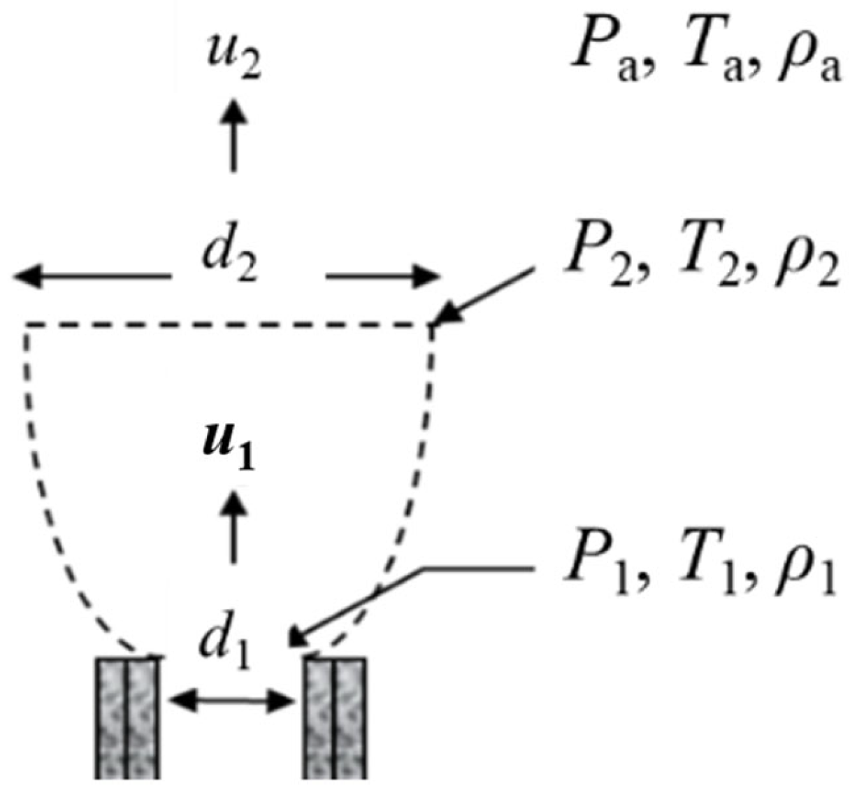
Momentum conservation equations

The momentum equations in the x, y, and z directions are given as

$$\mathsf{\nabla }\cdot \left(\rho u_{\mathrm{x}}\overrightarrow{u}\right)=\frac{\mathsf{\partial }p}{\mathsf{\partial }x}+\frac{\mathsf{\partial }{\tau }_{\mathrm{xx}}}{\mathsf{\partial }x}+\frac{\mathsf{\partial }{\tau }_{\mathrm{yx}}}{\mathsf{\partial }y}+\frac{\mathsf{\partial }{\tau }_{\mathrm{zx}}}{\mathsf{\partial }z}+\rho f_{\mathrm{x}}$$

(2)

$$\mathsf{\nabla }\cdot \left(\rho u_{\mathrm{y}}\overrightarrow{u}\right)=\frac{\mathsf{\partial }p}{\mathsf{\partial }y}+\frac{\mathsf{\partial }{\tau }_{\mathrm{xy}}}{\mathsf{\partial }x}+\frac{\mathsf{\partial }{\tau }_{\mathrm{yy}}}{\mathsf{\partial }y}+\frac{\mathsf{\partial }{\tau }_{\mathrm{zy}}}{\mathsf{\partial }z}+\rho f_{\mathrm{y}}$$

(3)

$$\mathsf{\nabla }\cdot \left(\rho u_z\overrightarrow{u}\right)=\frac{\mathsf{\partial }p}{\mathsf{\partial }z}+\frac{\mathsf{\partial }{\tau }_{\mathrm{xz}}}{\mathsf{\partial }x}+\frac{\mathsf{\partial }{\tau }_{\mathrm{yz}}}{\mathsf{\partial }y}+\frac{\mathsf{\partial }{\tau }_{\mathrm{zz}}}{\mathsf{\partial }z}+\rho f_z$$

(4)

where τ_ii (i = x, y, z) is the component of viscous stress, and Pa; f_i(i = x, y, z) is the unit mass force component, in m/s⁻².

(3)

Energy conservation equation

$$\frac{\mathsf{\partial }}{\mathsf{\partial }t}[\overrightarrow{u}(\rho E+p)]=\frac{\mathsf{\partial }}{\mathsf{\partial }{x}_{\mathrm{i}}}{k}_{eff}\mathsf{\nabla }T-\sum _{\mathrm{j}}{h}_{\mathrm{j}}{J}_{\mathrm{j}}+\left({\tau }_{eff}\cdot \overrightarrow{u}\right)+S_{\mathrm{h}}$$

(5)

where K_eff is effective thermal conductivity, W·m⁻¹·K⁻¹; h is enthalpy, J kg⁻¹, and enthalpy J is diffusion flux.

Select the DO model for thermal radiation calculation, and the radiation equation at position r along the direction s is [17]

$$\mathsf{\nabla }\cdot (I(\overrightarrow{r},\overrightarrow{s})\overrightarrow{s})+\left(a+{\sigma }_{\mathrm{s}}\right)I(\overrightarrow{r},\overrightarrow{s})=a{n}^2\frac{\sigma T^4}{\pi }+\frac{{\sigma }_s}{4\pi }{\int }_0^{4\pi }I(\overrightarrow{r},\overrightarrow{s})\mathsf{\Phi }\left(\overrightarrow{s},\overrightarrow{s^{\prime }}\right)d{\mathsf{\Omega }}^{\prime }$$

(6)

where $\overrightarrow{r}$ is position vector; $\overrightarrow{S}$ is directional vectors; $\overrightarrow{s^{\prime }}$ is scattering direction; $s$ is length; n is refractive index; σ_s is scattering coefficient; σ is Stephen Boltzmann constant; I is radiation intensity, size depends on location and direction; T is temperature; Φ is phase function; and Ω′ is spatial solid angle.

As for spectral radiation intensity, I($\overrightarrow{r}$,$\overrightarrow{s}$) radiation propagation equation is

$$\mathsf{\nabla }\cdot \left(I_{\lambda }(\overrightarrow{r},\overrightarrow{s})\overrightarrow{s}\right)+\left(a_{\lambda }+{\sigma }_{\mathrm{s}}\right)I_{\lambda }(\overrightarrow{r},\overrightarrow{s})=a_{\lambda }{n}^2{I}_{\mathrm{b}\lambda }+\frac{{\sigma }_{\mathrm{s}}}{4\pi }{\int }_0^{4\pi }{I}_{\lambda }(\overrightarrow{r},\overrightarrow{s})\mathsf{\Phi }\left(\overrightarrow{s},\overrightarrow{s^{\prime }}\right)d{\mathsf{\Omega }}^{\prime }$$

(7)

where λ is radiation wavelength; a_λ is spectral absorption coefficient; I_bλ is blackbody radiation intensity determined by Planck’s law; the scattering coefficient, scattering phase function, and refractive index are assumed to be wavelength independent. The non gray body DO radiation model divides the entire radiation spectral band into N (long) bands, which do not need to be continuous or equidistant. The wavelength interval is given by the user, and this interval is the value (refractive index) in vacuum. The radiation propagation equation integrates wavelengths across all wavelength ranges to obtain the transport equation for I_λΔλ. Radiation heat is contained within each wave band. Within each wave band Δλ, considered as blackbody radiation, the blackbody radiation per unit solid angle [18] is

$$\left[F\left(0\to n{\lambda }_{2}T\right)-F\left(0\to n{\lambda }_{1}T\right)\right]n^2\frac{\sigma T^4}{\pi }$$

(8)

where F(0→nλT) is the radiation of a blackbody in the wavelength range of 0~λ at temperature T in a medium with a refractive index of n; λ₁, λ₂ is the boundary of the wave band.

The total radiation intensity $I\left(\overrightarrow{r},\overrightarrow{s}\right)$ at direction $\overrightarrow{s}$ and position $\overrightarrow{r}$ is

$$I(\overrightarrow{r},\overrightarrow{s})=\sum _{\mathrm{k}}{I}_{\lambda \mathrm{k}}(\overrightarrow{r},\overrightarrow{s})\mathsf{\Delta }{\lambda }_{\mathrm{k}}$$

(9)

where summation is performed over the entire wavelength range. The boundary conditions for non gray body DO models are based on the boundary conditions of wave bands (i.e., each wave band corresponds to a boundary condition), and within a wave band, the handling of its boundary conditions is the same as that of gray body DO models.

(4)

Component transport equation

When a flowing fluid consists of more than one component, each component must satisfy the continuity equation. Accordingly, the conservation equation for component k can be derived as [17]

$$\nabla \left(\rho \overrightarrow{u}{c}_{\mathrm{k}}\right)=\nabla \left(D_{\mathrm{k}}grad\left(\rho c_{\mathrm{k}}\right)\right)+S_{\mathrm{k}}$$

(10)

where c is the volume fraction and S is the generation rate.

Through a comparative analysis of the applicability of various combustion models and the combustion characteristics of blowout jet flames, this study adopts a non-premixed combustion model to simulate blowout jet fires. The combustion process is assumed to be fully burned, and the combustion products are CO₂ and H₂O without any intermediate products. The probability density functional (PDF) solution method is employed to solve the non-premixed combustion model.

2.1.2. Turbulence Model

After the blowout ignites, the jet flame becomes a highly turbulent fluid, necessitating the use of a turbulence model for characterization. The turbulence model employed in this study is the Reynolds-averaged Navier–Stokes method, specifically the realizable k − ε model. This method is highly applicable to engineering problems, such as blowout jet flames, and does not require considerable computational resources. The mathematical representation of the model is given as [19]

$$\frac{\mathsf{\partial }K}{\mathsf{\partial }\tau }+\frac{\mathsf{\partial }(\rho \overline{u_{\mathrm{j}}}K)}{\mathsf{\partial }{x}_{\mathrm{j}}}=\frac{\mathsf{\partial }}{\mathsf{\partial }{x}_{\mathrm{j}}}\left[{\alpha }_{\mathrm{K}}\left(\mu +\frac{{\mu }_{\mathrm{t}}}{{\sigma }_{\mathrm{K}}}\right)\frac{\mathsf{\partial }K}{\mathsf{\partial }{x}_{\mathrm{j}}}\right]+G_{\mathrm{K}}+G_{\mathrm{b}}-\rho \epsilon -Y_{\mathrm{M}}$$

(11)

where σ_K is the turbulent kinetic energy corresponding to the Prandtl number in which σ_K = 1.0, G_b is the turbulent kinetic energy term generated by buoyancy, and G_K is the turbulent kinetic energy term generated by the mean velocity.

$$\begin{array}{l}\frac{\mathsf{\partial }(\rho \epsilon )}{\mathsf{\partial }\tau }+\frac{\mathsf{\partial }(\rho {\overline{u}}_{\mathrm{j}}\epsilon )}{\mathsf{\partial }{x}_{\mathrm{j}}}=\frac{\mathsf{\partial }}{\mathsf{\partial }{x}_{\mathrm{j}}}\left[{\alpha }_{\mathsf{\epsilon }}\left(\mu +\frac{{\mu }_{\mathrm{t}}}{{\sigma }_{\mathsf{\epsilon }}}\right)\frac{\mathsf{\partial }\epsilon }{\mathsf{\partial }{x}_{\mathrm{j}}}\right]+\\ \rho C_1\overline{S}\epsilon -C_2\rho \frac{{\epsilon }^2}{K+\sqrt{v\epsilon }}-C_{\mathsf{\epsilon }1}\frac{{\epsilon }^2}{k}{C}_{\mathsf{\epsilon }3}{G}_{\mathrm{b}}\end{array}$$

(12)

where σ_ε is the Prandtl number corresponding to the turbulent dissipation rate, σ_ε = 1.3; C_ε1 is a constant, C_ε1 = 1.44; when the shear flow with flow velocity is in the same direction as gravity, C_ε3 = 1; otherwise, C_ε3 = 0.

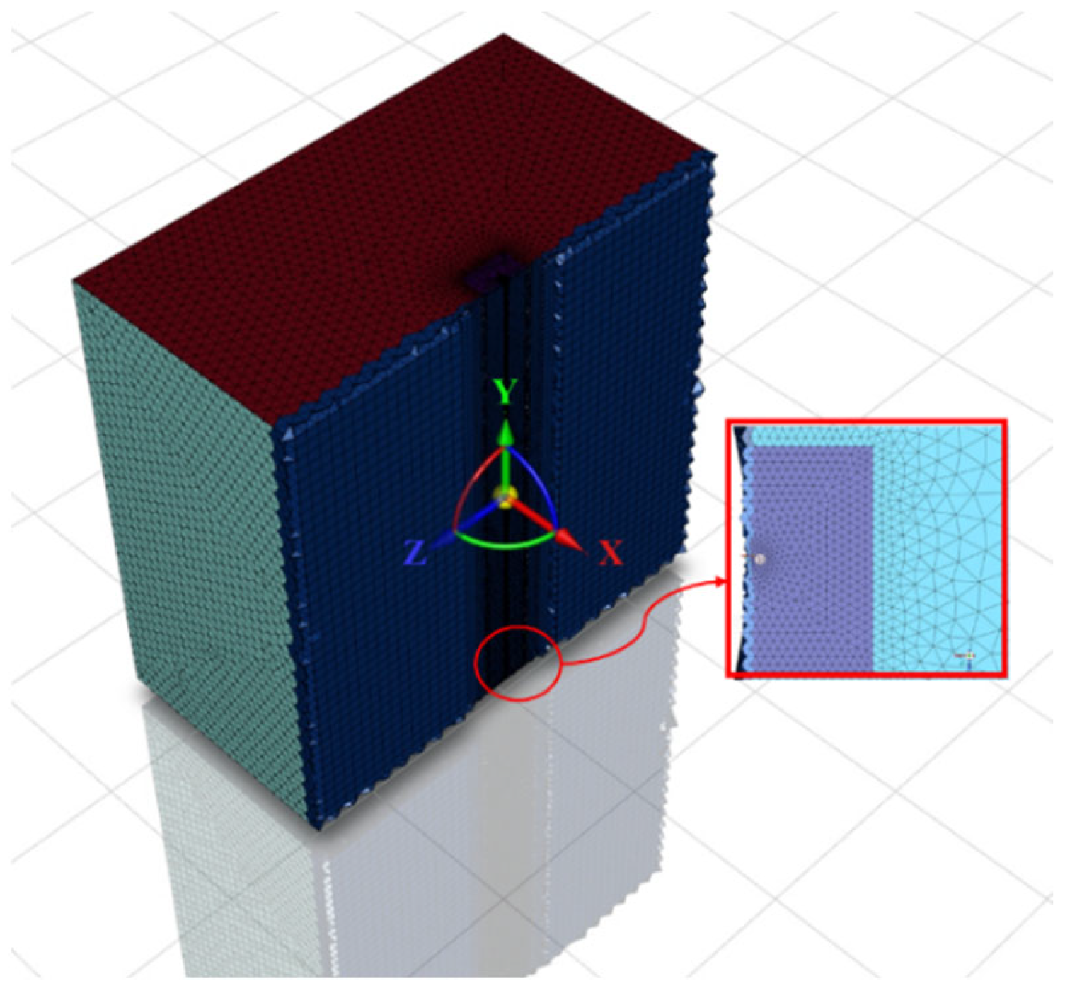
2.1.3. Boundary Conditions and Solution Method

The calculation domain is determined to be a cubic model with dimensions of 3 × 3 × 3 m. Geometric modeling is performed using SpaceClaim software 2023. A methane nozzle is positioned at the bottom center of the model, with the nozzle located 734 mm above the ground. The three-dimensional model is illustrated in Figure 1, where the Y direction indicates the direction of the methane jet flame combustion.

Based on the experimental conditions, the numerical simulation boundary conditions are determined as follows. Methane is introduced as a mass flow inlet with a pressure of 0 Pa. The boundary conditions for the nozzle and ground are set as non-slip wall surfaces, and the wall heat transfer mode is chosen as radiation. Other boundary conditions are set as pressure outlets with a pressure of atmospheric pressure.

To determine the methane inlet, the phenomenon of underexpanded jet flow at the nozzle must be considered. This leads to a decrease in the gas density, an increase in the velocity, and a decrease in the temperature at the nozzle. Consequently, the temperature and pressure of the gas flow core from the wellhead to the Mach disk are much lower than the ambient air temperature and pressure, and a complex shockwave structure is formed just outside the wellhead over a short distance. Therefore, for calculations of blowout jet flow processes, simplifying the actual complex underexpanded jet flow process and utilizing the theory of low-pressure leak jet flow to provide an “equivalent” inlet condition for blowouts are necessary. Birch et al. introduced the concept of a “pseudo-diameter’ and proposed the “virtual nozzle” model to analyze the attenuation of gas concentration along the centerline during high-pressure natural gas leakage processes. As Figure 2 shows, this model assumes that the high-pressure gas passing through the virtual nozzle has the same mass flow rate as that passing through the actual nozzle. At the virtual nozzle, the gas pressure and temperature are equal to the atmospheric pressure and temperature of the surrounding environment, respectively. The expansion process of the high-pressure gas is approximated as adiabatic and isentropic. The mass conservation equation for the jet gas flow from the nozzle to the virtual nozzle is

$${\rho }_1{u}_1{A}_1={\rho }_2{u}_2{A}_2$$

(13)

where u₁ is gas velocity at the wellhead, m·s⁻¹; u₂ is the equivalent gas velocity at the virtual nozzle, m·s⁻¹; A₂ is the equivalent area at the virtual nozzle, m²; A₁ is the wellhead area, m²; and ρ₂ is the equivalent gas density at the virtual nozzle, kg·m⁻³.

The momentum conservation equation is

$${\rho }_1{u_1}^2{A}_1={\rho }_2{u_2}^2{A}_2+\left(p_2-p_1\right)A_1$$

(14)

By simultaneously solving Equations (9) and (10), we can obtain the gas velocity at the virtual nozzle as

$$u_2=u_1-\frac{\left(P_2-P_1\right)}{{\rho }_1{u}_1}$$

(15)

The diameter of the virtual nozzle is

$$d_2=d_1\sqrt{\frac{u_1{\rho }_1}{u_2{\rho }_2}}$$

(16)

The pressure–velocity decoupling scheme adopts a Coupled algorithm. To improve computational accuracy, prevent numerical divergence, and maintain upwind properties, the convective terms in the transport equations are discretized using the second-order accurate quadratic upwind interpolation of convective kinematics (QUICK) scheme.

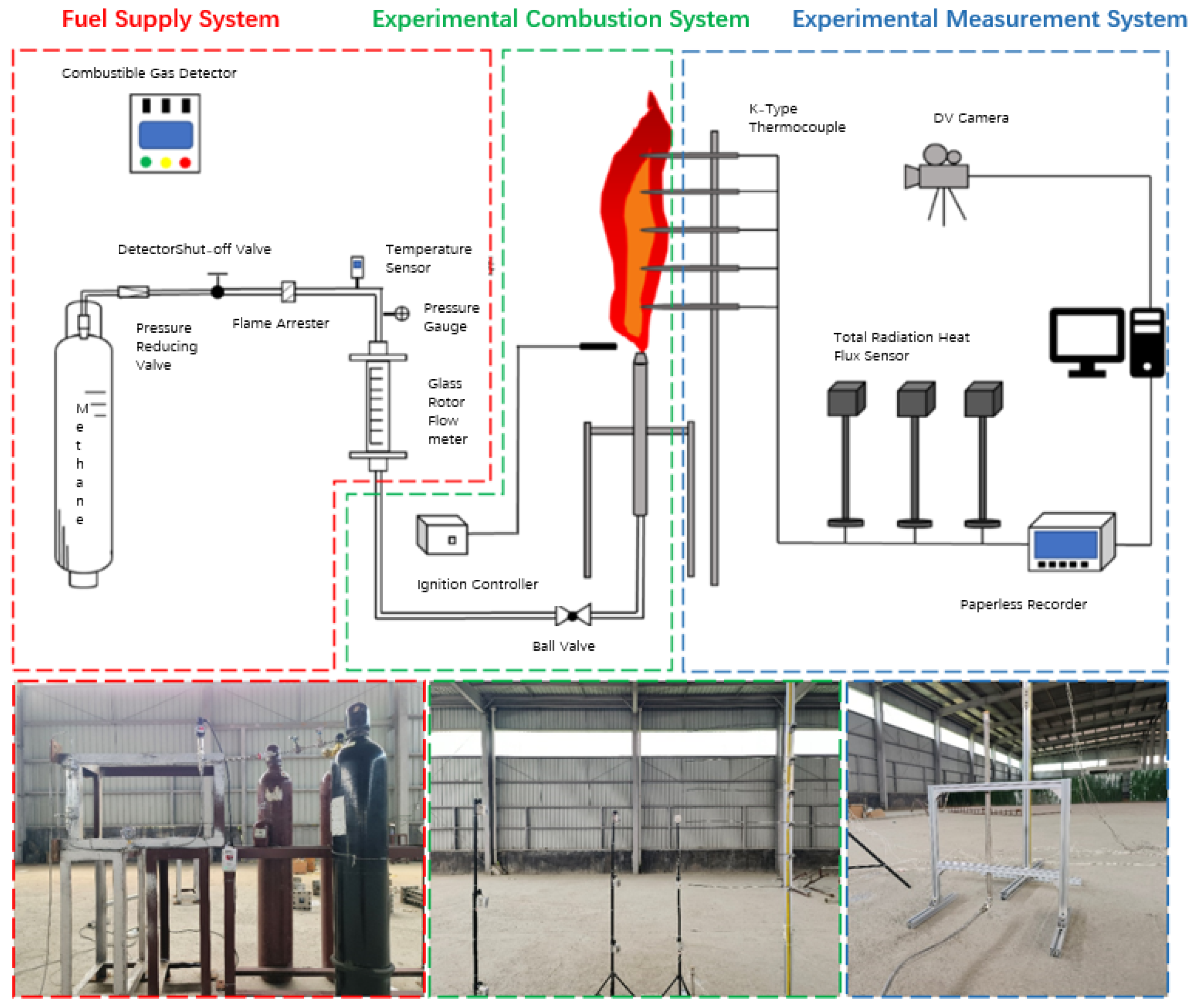
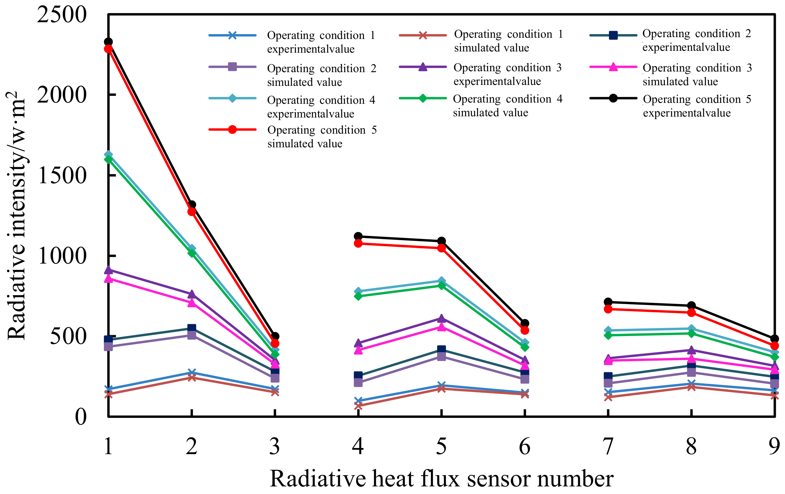
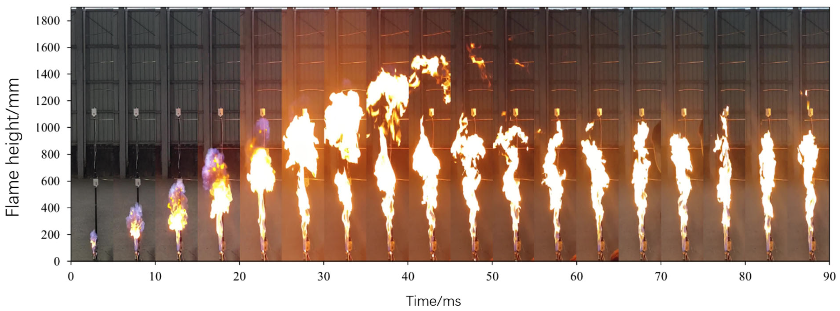
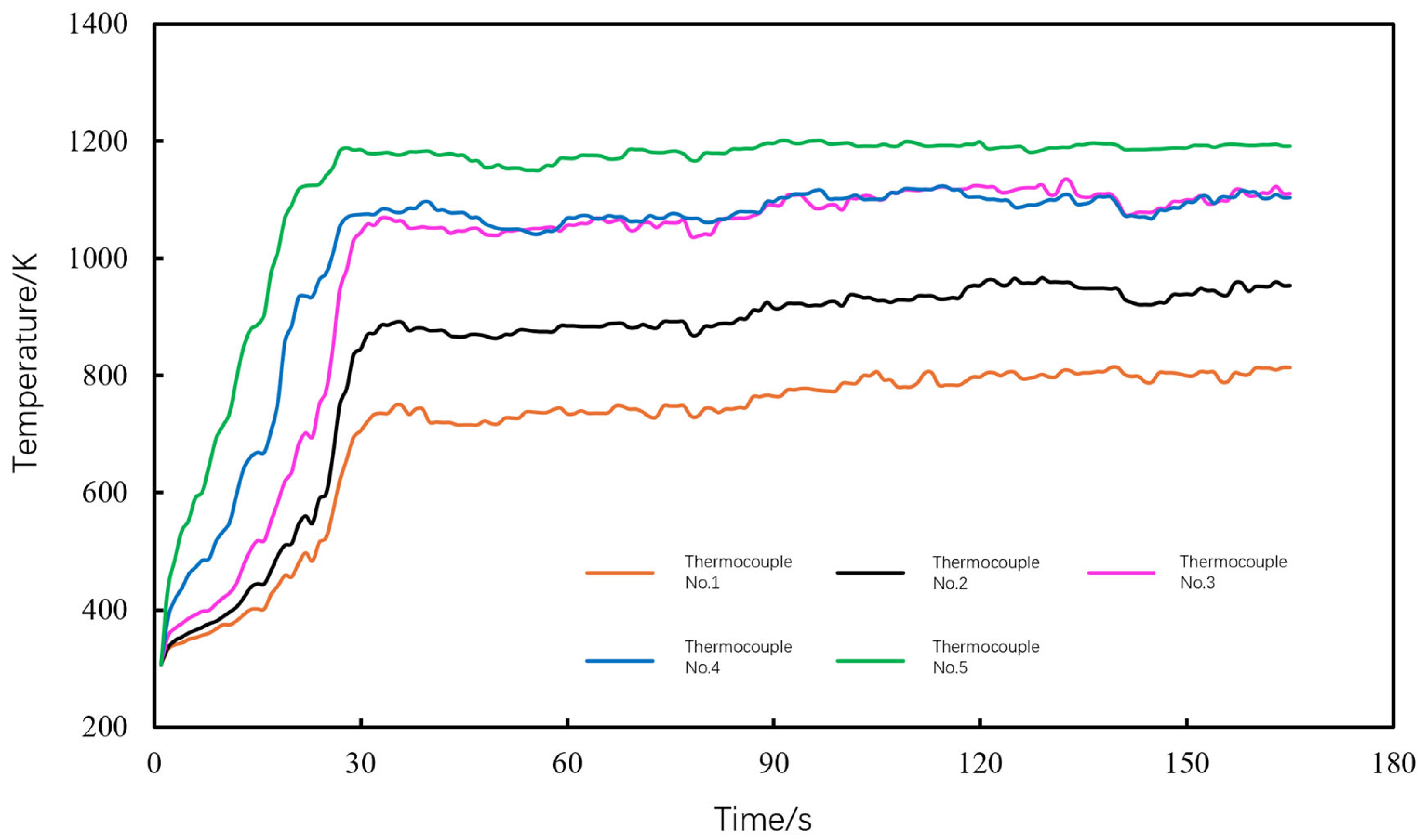
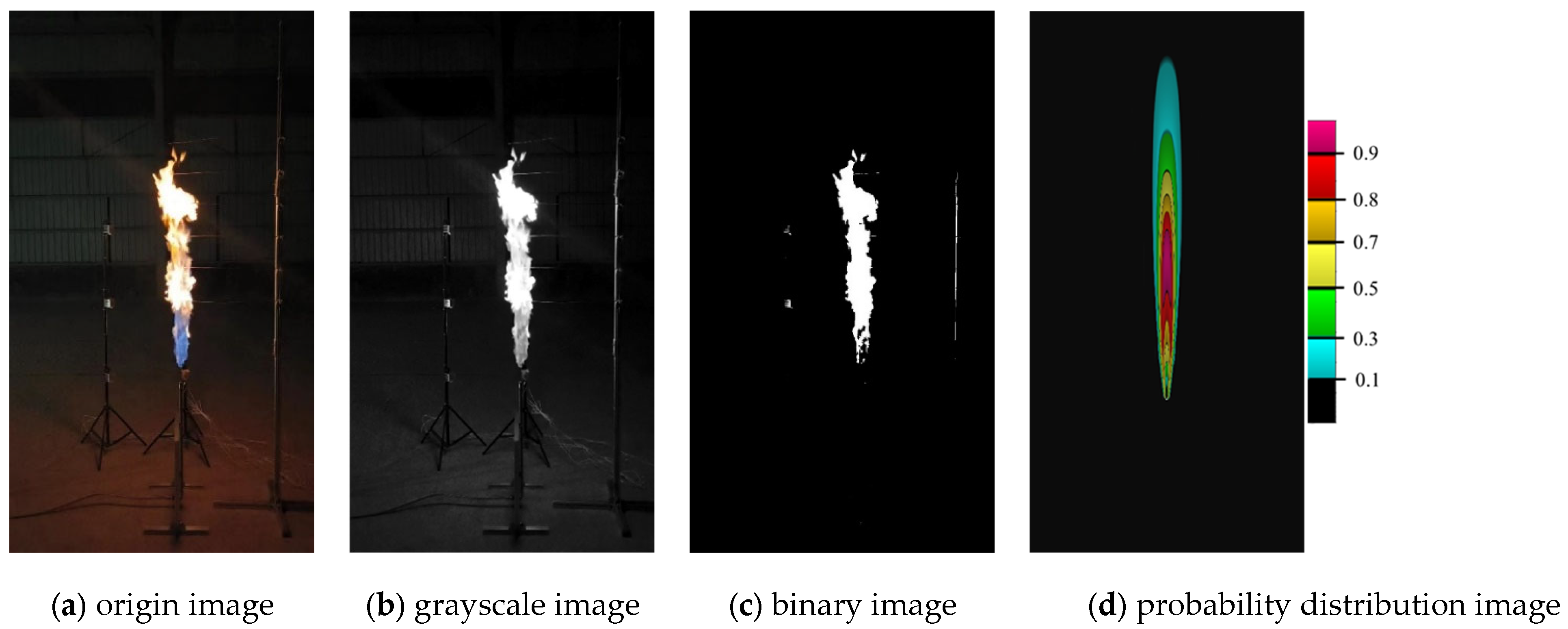
2.2. Model Verification

To ensure the accuracy of the simulation results, validating the numerical model previously established using experimental data is necessary. The model validation section primarily uses experimental and simulation data for nozzle diameters of 10 mm and methane volume flow rates of 3.6, 2.8, 2.0, 1.2, and 0.4 m³/h.

The experimental setup for the jet flame study is conducted in an open environment and consists primarily of fuel supply, experimental combustion, and experimental measurement systems. Figure 3 shows a schematic and photographs of the experimental setup. The thermocouples are arranged starting from a distance of 2.36 m above the ground, labeled as “1”, and then placed at intervals of 20 cm downward, totaling six thermocouples. The thermal radiometers are divided into three groups: radiometers 1, 2, and 3, located 80 cm from the nozzle at heights of 185, 125, and 65 cm, respectively. Radiometers 4–9 are positioned 100 and 130 cm away from the nozzle, with heights similar to those of radiometers 1, 2, and 3.

The experimental focus of this study primarily concerns the jet flame height, flame center temperature, and the distribution of thermal radiation around the flame, with the method for determining whether the jet flame reaches a stable state being the absence of significant changes in flame morphology and a tendency of the flame center temperature to stabilize. As shown in Figure 4 and Figure 5, after ignition, both flame height and temperature gradually increase and eventually stabilize, with the temperature stabilization process taking approximately 30 s. Due to the gradual heating of the thermocouple to match the actual flame temperature, it takes a considerable amount of time. Therefore, data collection in this experiment began 40 s after ignition, with continuous recording for 1 min to observe the steady-state combustion process of the methane jet under this operating condition.

In this experiment, the probability distribution contour method is employed to characterize the geometric morphology of the jet flame, as illustrated in Figure 6. Initially, MATLAB software r2023a is utilized to convert the colored images of the jet flame into grayscale images. Subsequently, the grayscale images are further converted into binary images to obtain pixel matrices for the flame and non-flame areas. Finally, calculations are performed by superimposing all of the images. Based on the frequency of occurrence of flame morphology, a probability distribution map of the flame area is obtained. The portion with a probability greater than 0.5 is selected as the true morphology of the methane jet flame under the experimental conditions, thus determining the flame height under different experimental conditions.

In order to simulate different operating conditions, five sets of experiments were designed with methane volumetric flow rates of 0.4 m³/h, 1.2 m³/h, 2.0 m³/h, 2.8 m³/h, and 3.6 m³/h as

Table 1. Operating conditions in combustion experiment.

Operating condition	1	2	3	4	5
Methane volumetric flow rate, m3·h−1	0.4	1.2	2.0	2.8	3.6

shows. The following are the comparative validation results for the experimental and simulated data.

Figure 7 shows a comparison of the experimental and simulated values of the methane jet flame heights under the five scenarios. The average error between the simulated and experimental values was 3.61%. Figure 8 and Figure 9 present a comparison of the experimental and simulated values of the methane jet flame temperatures and thermal radiation intensities under the five scenarios, respectively. The figures show that the trends of the simulated flame centerline temperature and thermal radiation intensity matched well with the experimental data. The relative errors between the simulated and experimental values for the flame temperature and radiation intensity were 16.94% and 9.54%, respectively. These errors meet the requirements of industrial applications [20], thus confirming the feasibility and accuracy of the simulation method.

3. Simulation Analysis of Jet Flame Combustion Characteristics under Blowout Conditions

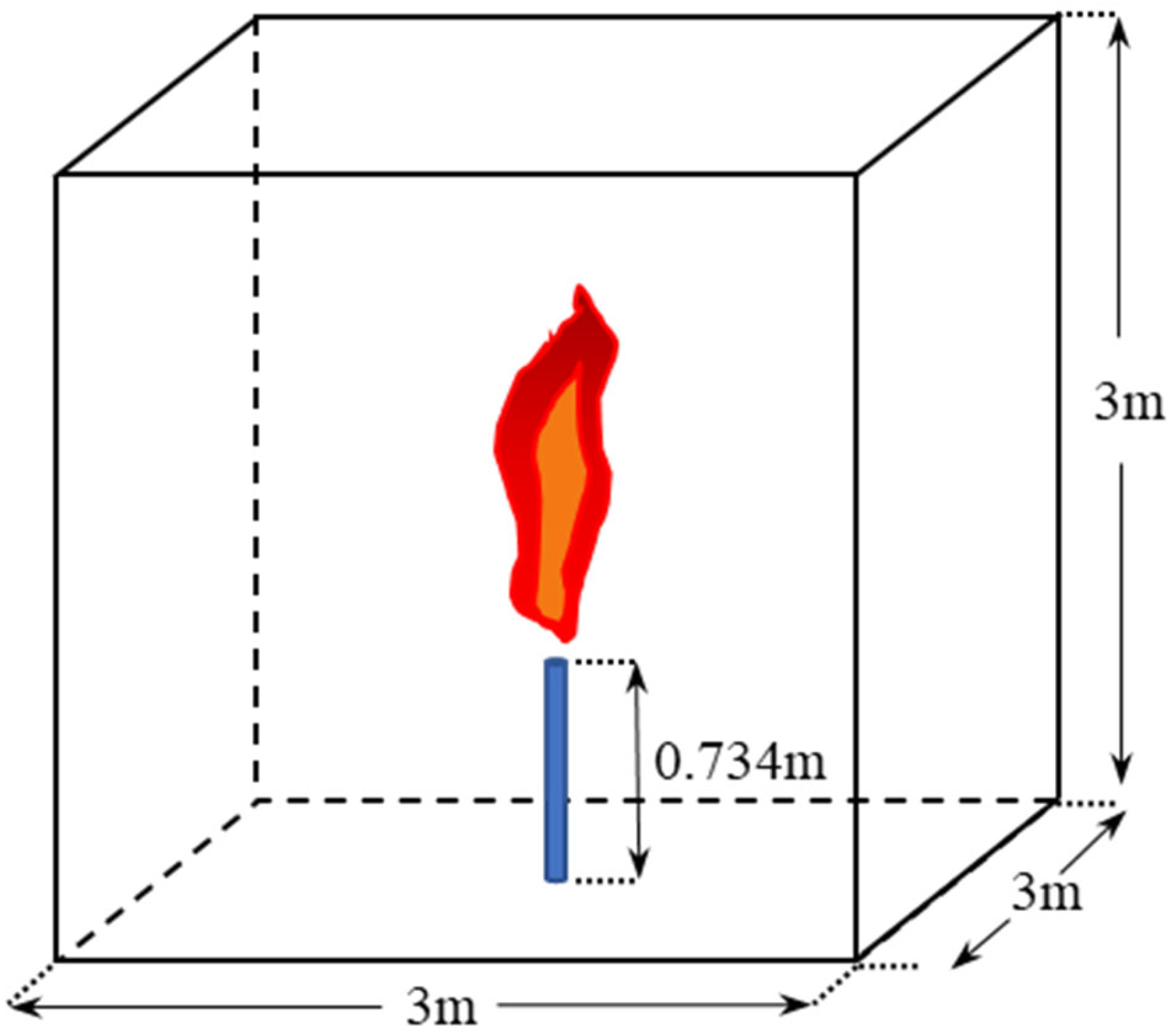
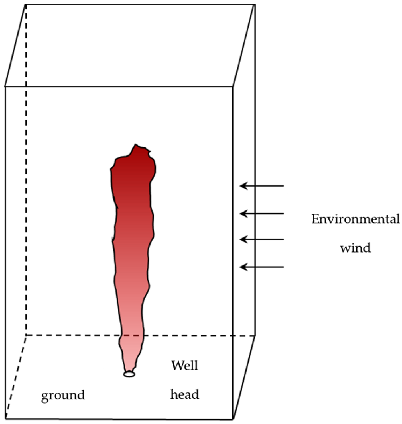
3.1. Blowout Fire Physical Model

To capture accurately the combustion characteristics of jet flames under on-site blowout conditions, a large-scale physical model was established for simulation calculations based on the accuracy validation of a small-scale model. The computational domain of this model was a cubic region with dimensions of 80 m in length and width and 150 m in height, as shown in Figure 10. Given that the gas flow and combustion chemical reactions were primarily concentrated in the region directly above the blowout wellhead, this area was treated with a refined mesh using a small-scale grid. Through grid-independence testing, a mesh division method consisting of 1.5 million grid cells was selected for the numerical simulation. Figure 11 illustrates the grid divisions.

The pressure–velocity decoupling scheme adopts the Coupled algorithm. To enhance computational accuracy and avoid numerical divergence while maintaining upwind characteristics, the convective terms of the transport equations are discretized using the second-order accurate QUICK scheme.

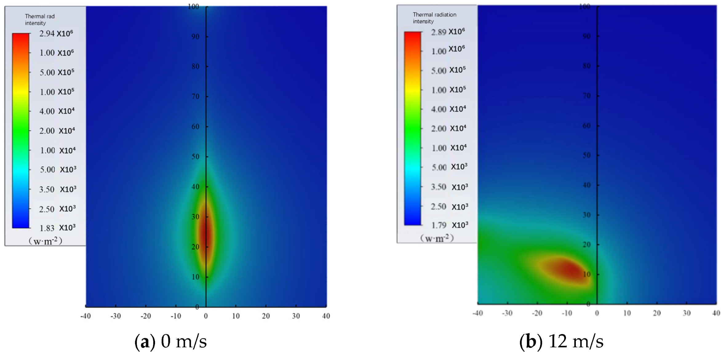
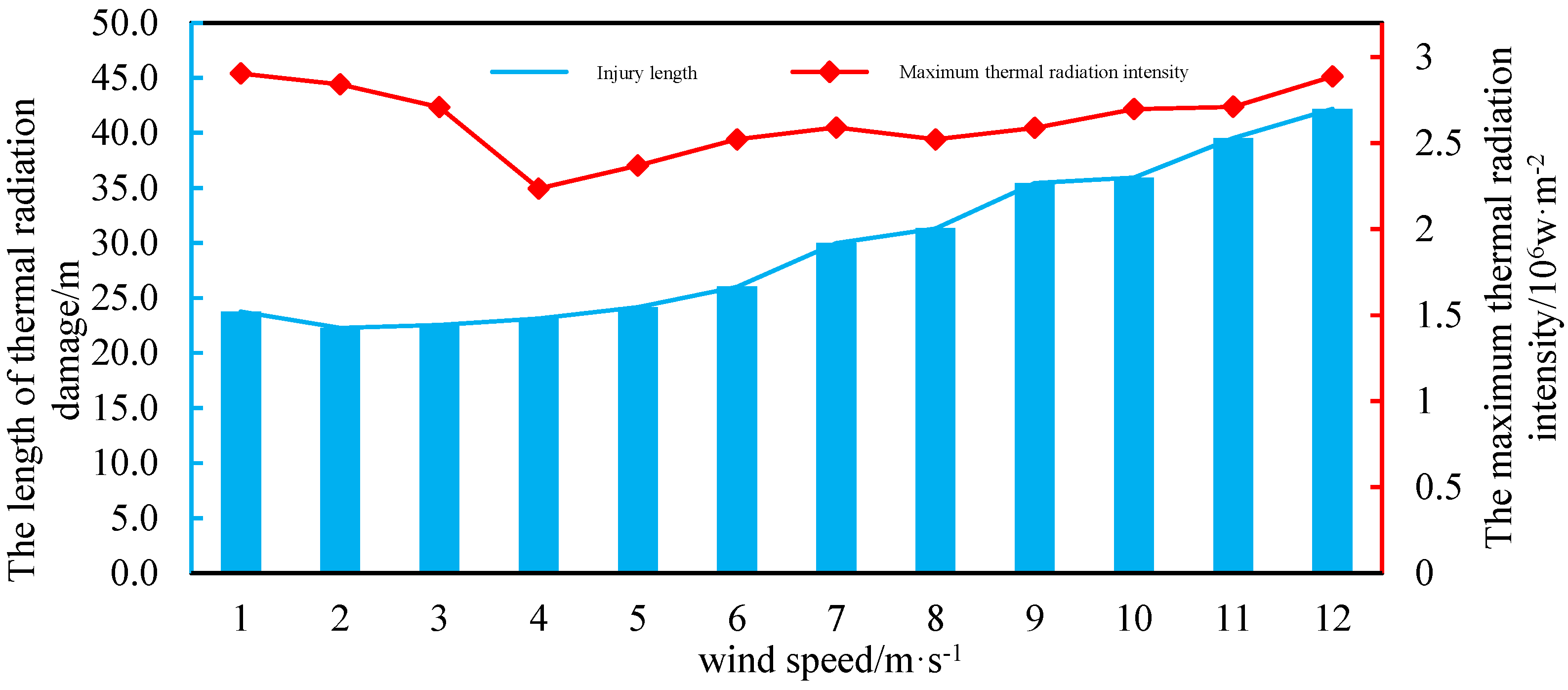
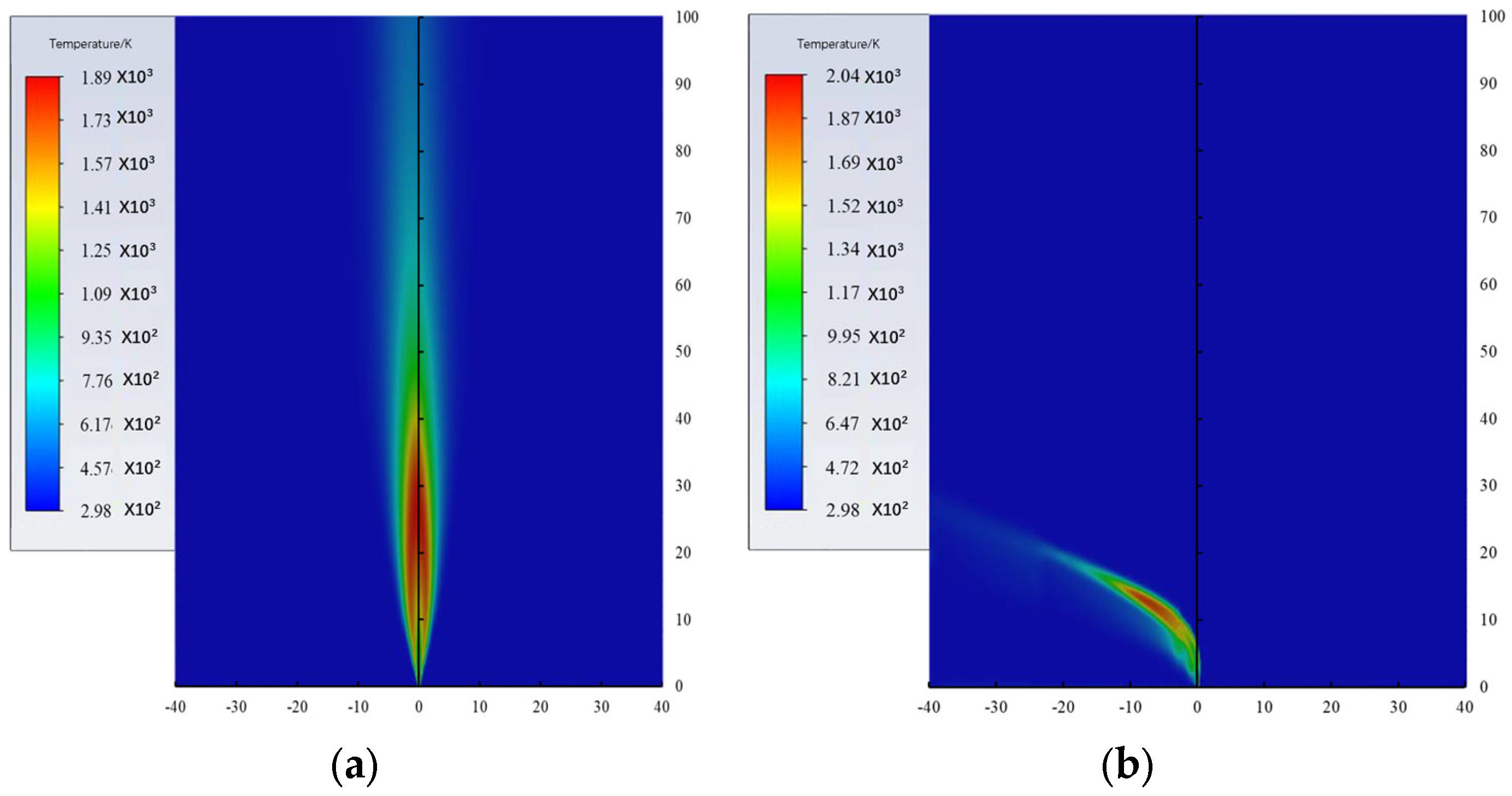
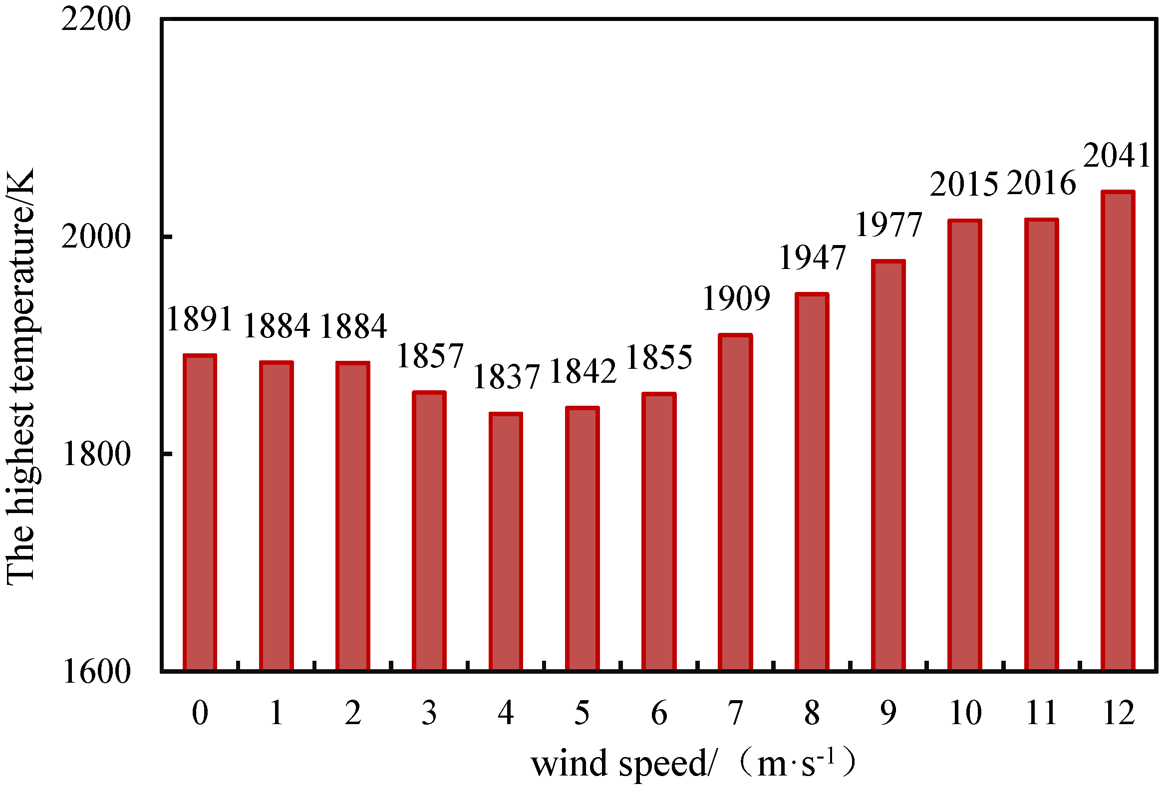
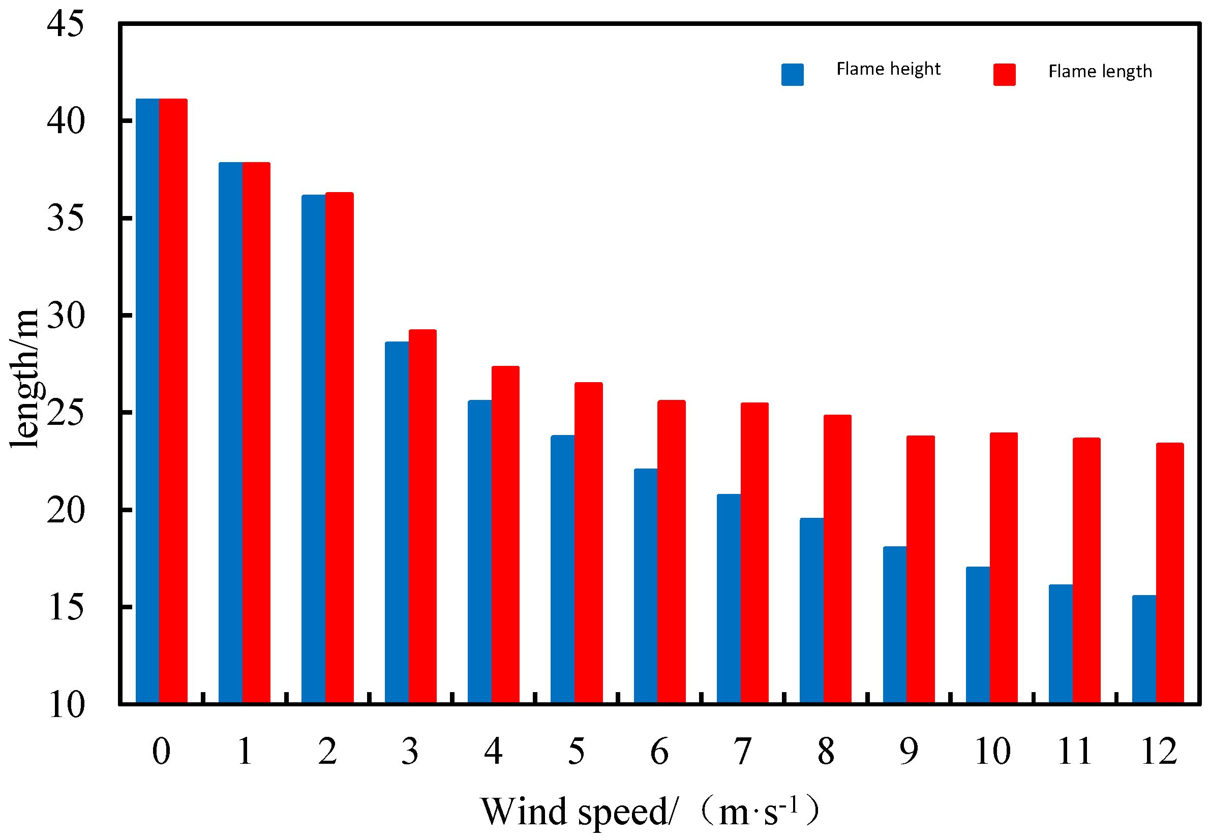
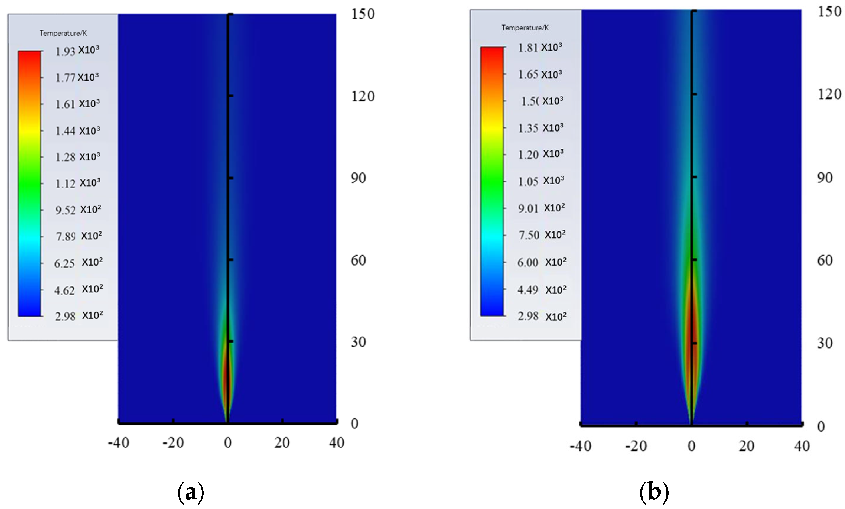
3.2. Effects of Wind Speed on the Combustion Characteristics of Blowout Jet Flames

The wind speed has a significant effect on the morphology and combustion characteristics of blowout jet flames. Based on the assumption of a mass flow rate of 10 kg/s for the blowout natural gas, wellbore diameter of 20 mm, and ambient pressure of standard atmospheric pressure, the effects of varying crosswind speeds (0–12 m/s) on the temperature field, with the environmental wind blowing in from the right side of the experimental setup, with consistent direction and uniform speed that does not vary with height, on thermal radiation intensity distribution, and on flame height of blowout jet flames were studied.

(1)

Effects of wind speed on the flame temperature field

Figure 12 shows the temperature field contours of the jet flame, where the temperature along the central axis of the flame first increased and then decreased. In both regions, the bottom of the jet flame consisted mainly of unreacted gas, whereas the top consisted mainly of combustion products with lower temperatures. The middle part of the flame was the core area of the combustion reaction, where the flame temperature was the highest. With increasing crosswind speed, the flame temperature decreased more rapidly. At lower wind speeds, the gas at the nozzle could not fully react, and the airflow carried the gas to burn in distant areas, resulting in a greater distribution range of the flame temperature field. At higher wind speeds, the intensified airflow increased the air entrainment rate of the jet flame, providing sufficient oxygen for the combustion of blowout combustible gases and leading to more intense combustion chemical reactions. However, crosswinds could scatter some of the fuel, resulting in a lower combustion range of the blowout jet flame as compared with no-wind conditions.

As Figure 13 shows, the maximum temperature of the blowout jet flame decreased before the crosswind speed reached 4 m/s. However, as the crosswind speed further increased, the maximum temperature of the blowout jet flame increased. Lower crosswind speeds dissipated the heat generated by the combustion reaction of the jet gas, resulting in a decrease in temperature. As the wind speed continued to increase, the airflow provided sufficient oxygen, leading to more complete and intense combustion and causing the temperature to increase.

(2)

Effects of wind speed on the flame radiation field

Figure 14 shows the contour maps of the thermal radiation intensity at the center of the flame under no-wind conditions and a crosswind speed of 12 m·s⁻¹. Under the effects of crosswind speed, the thermal radiation field of the blowout jet flame shifted downward in the downwind direction. In addition, as the wind speed increased, the core area of the thermal radiation moved closer to the ground, and the distribution range of the thermal radiation above the flame diminished.

Figure 15 illustrates the maximum thermal radiation intensity and length of the thermal radiation damage under different wind speed conditions of the blowout jet flame. The maximum thermal radiation intensity of the flame corresponds to the highest flame temperature generated by the blowout flame. Under a crosswind speed of 4 m/s, the maximum thermal radiation intensity at the center of the jet flame was the lowest, approximately 2.24 × 10⁶ W/m². By contrast, under a crosswind speed of 12 m/s, the maximum thermal radiation intensity at the center of the jet flame was the highest, approximately 4.22 × 10⁶ W/m². Under conditions of lower crosswind speeds, the safe distance from thermal radiation damage remained largely consistent with the no-wind conditions at approximately 23 m. However, as the wind speed further increased, the safe distance increased. When the wind speed reached 12 m/s, the thermal radiation damage zone of the jet flame significantly exceeded the boundaries of the simulation model.

(3)

Effects of wind speed on flame height

Figure 16 shows the variations in flame length of the well blowout jet flame with lateral wind speed. At lateral wind speeds of 3 m/s, the flame length was nearly equal to the flame height because the well blowout jet flame was mainly influenced by the initial momentum of the blowout. However, as the lateral wind speed further increased, the length of the well blowout jet flame became significantly greater than the flame height. In general, flame length decreased with increasing wind speed. This was because higher lateral wind speeds led to increased air pulsation rates and turbulence intensity, thereby enhancing the mixing between the blowout jet gas and surrounding air. This accelerated the dilution of the combustible gas, causing the gas concentration to decrease more rapidly and resulting in a reduction in the length of the jet flame with increasing lateral wind speed.

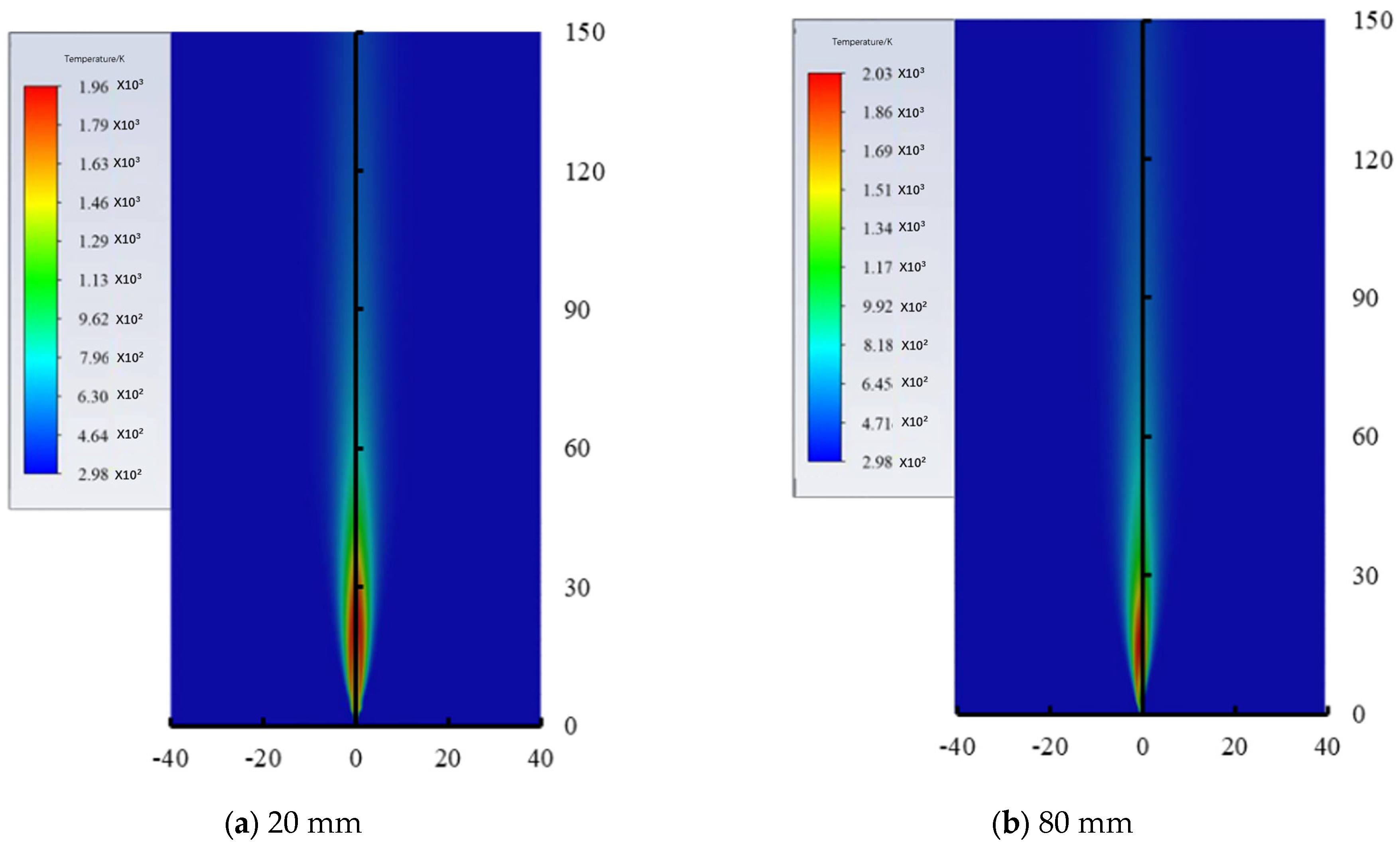
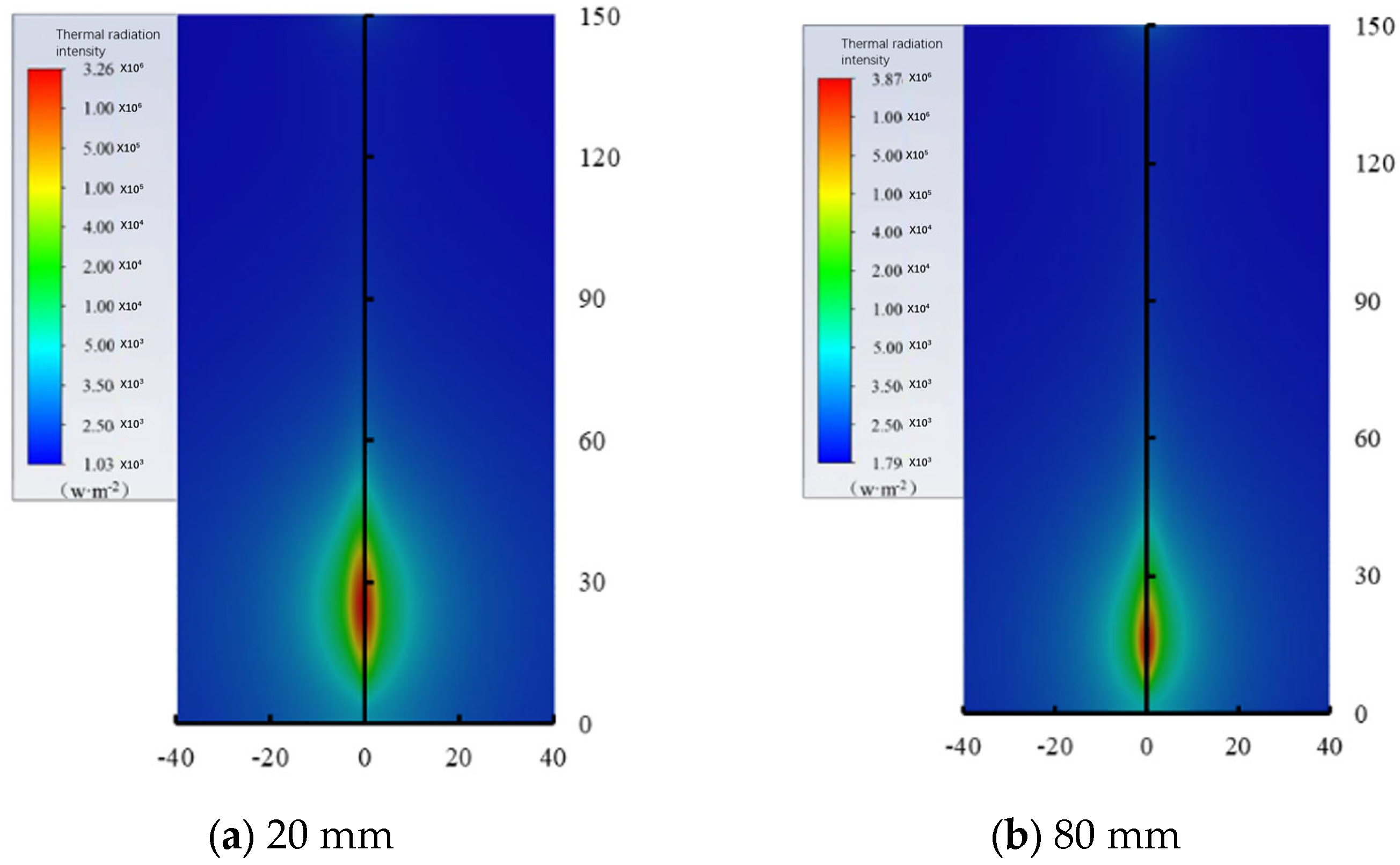
3.3. Effects of Blowout Gas Flow Rate on Blowout Jet Flame

The blowout gas flow rate determines the gas pressure and velocity at the wellhead. To investigate the effects of blowout gas flow rate on the morphology and thermal radiation of jet flames, simulations of blowout jet flames were conducted under no-wind conditions at different blowout gas flow rates (from 40 × 10⁴ to 170 × 10⁴ m³/d).

(1)

Effects of blowout gas flow rate on flame temperature field

Figure 17 illustrates the temperature distributions of the jet flames under different blowout gas flow rates. As the blowout gas flow rate increased, the pressure at the wellhead also increased. This resulted in a higher combustion rate of the gas after the blowout and an increased impact intensity of the jet flames, leading to a larger area being affected by the jet flames. Although an increased blowout gas flow rate resulted in a larger combustion area, no significant change in the maximum temperature of the jet flames was observed, which remained at approximately 1900 K.

(2)

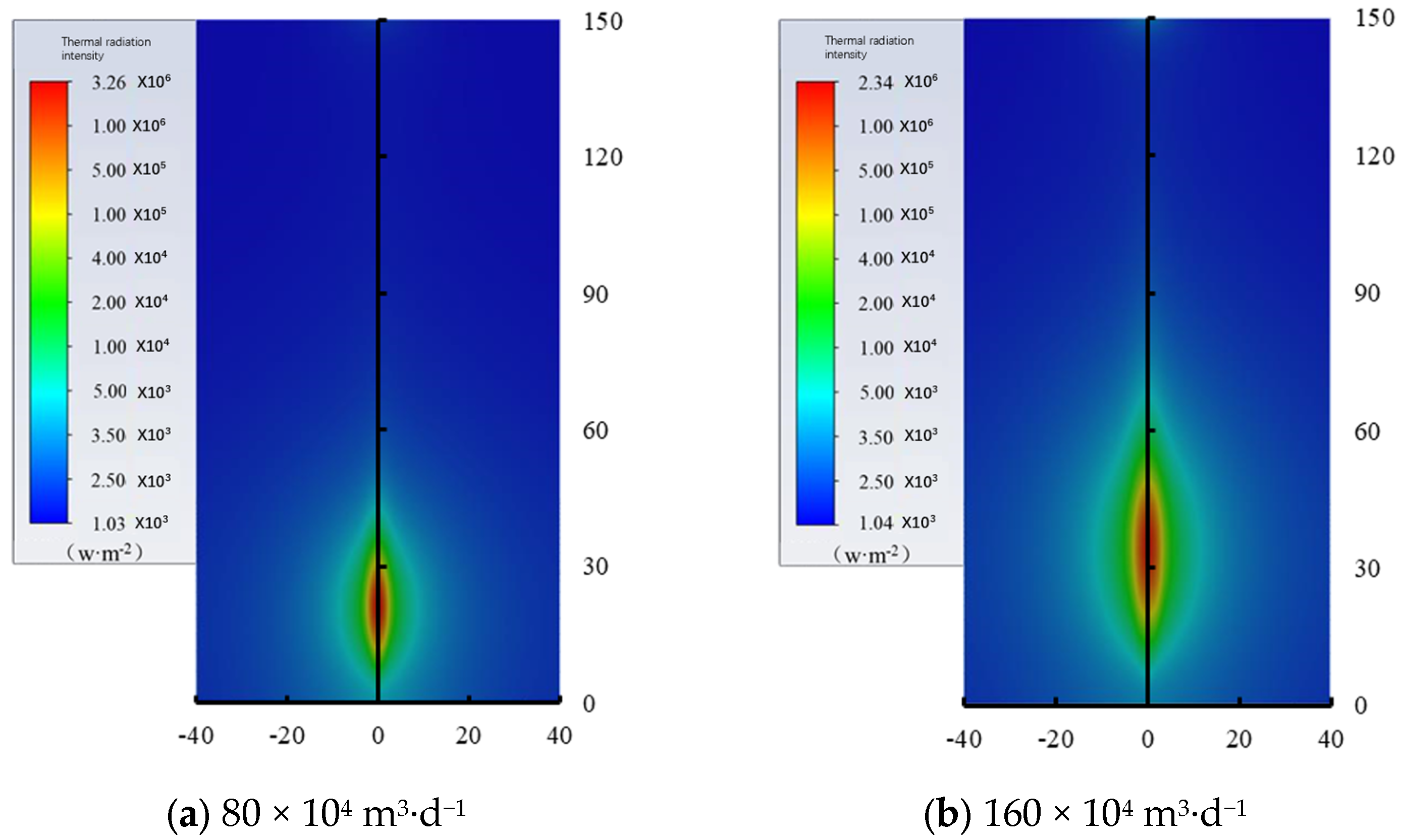
Effects of blowout gas flow rate on flame radiation field

Figure 18 shows the thermal radiation patterns of the jet flames under different blowout gas flow rates. As the blowout gas flow rate increased, the area affected by the thermal radiation increased. However, with an increase in the blowout gas flow rate, the maximum thermal radiation intensity decreased.

(3)

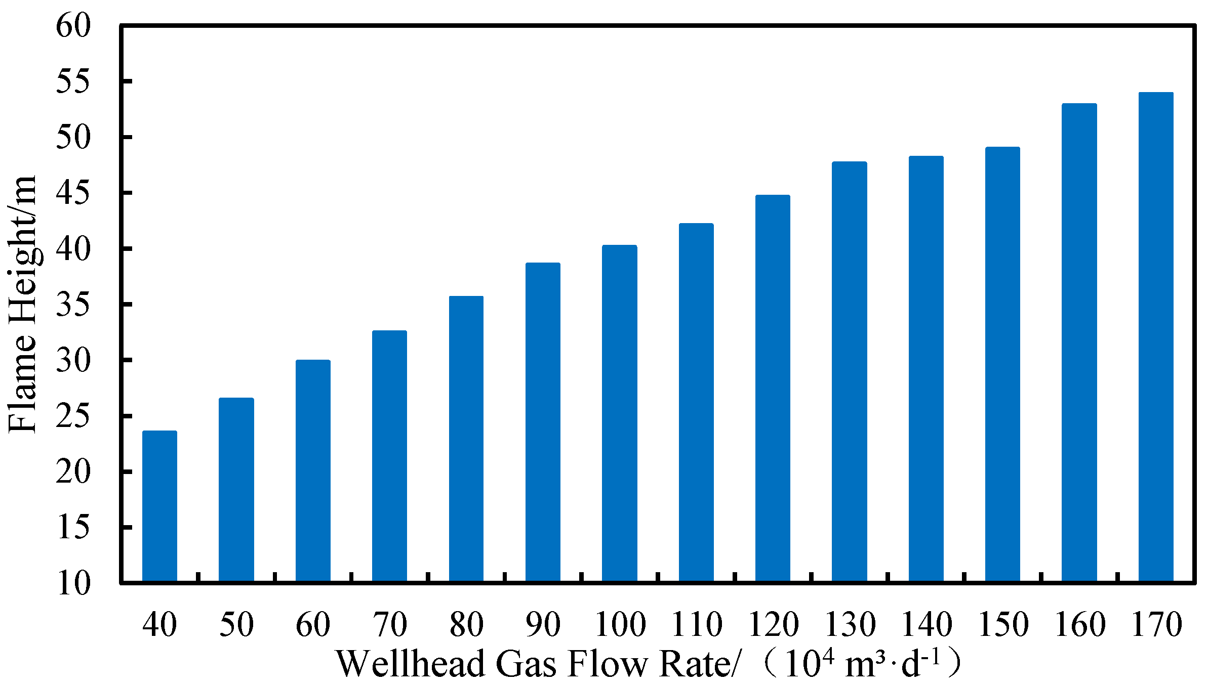
Effects of blowout gas flow rate on flame height

As Figure 19 shows, with an increase in the blowout gas flow rate, the flame height increased under unchanged conditions. The primary reason for this was that with the same nozzle diameter, the natural gas flow rate increased per unit time, resulting in a larger combustion volume and, in turn, a higher flame height.

3.4. Wellhead Size Effects on Blowout Jet Flame

To maintain other consistent conditions, simulations of the blowout jet flames were conducted under seven wellhead diameters ranging from 20 to 80 mm.

(1)

Effects of wellhead diameter on flame temperature field

Figure 20 illustrates the temperature distribution of the blowout jet flames with different wellhead diameters. When the wellhead diameter was large (80 mm), the initial kinetic energy of the gas at the wellhead was low, resulting in rapid velocity attenuation. Consequently, convective diffusion between the blowout natural gas and ambient air was slow. By contrast, when the wellhead diameter was small (20 mm), the initial kinetic energy of the gas at the wellhead was higher, leading to a faster convective diffusion between the blowout natural gas and ambient air. According to the gas combustion equilibrium relationship, an increase in wellhead diameter promotes combustion reactions. Therefore, under the same blowout gas volume, the core temperature area of the jet flame increased with the wellhead diameter.

(2)

Effects of wellhead diameter on flame radiation field

From the simulation results as shown in Figure 21, the thermal radiation distributions of blowout jet flames with different wellhead diameters are displayed. The radiation field cloud map analysis revealed that with an increase in the wellhead diameter, the area of thermal radiation hazard decreased.

(3)

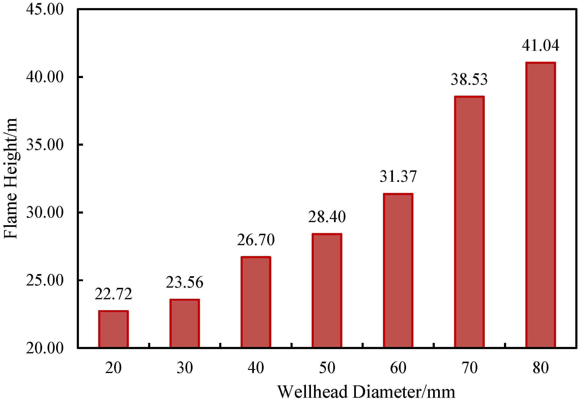
Effects of wellhead diameter on flame height

Figure 22 shows the numerical simulation results of variations in the flame height with different wellhead diameters. We observed that with an increase in the wellhead diameter, the height of the blowout jet flames increased. Based on the mass concentration of OH, it could be inferred that at a blowout gas flow rate of 10 kg/s and under a simulated flame height of 41.04 m, the flame height was the highest when the wellhead diameter was 20 mm.

4. Prediction Methods for Gas Flow Rate at the Wellhead under Blowout Conditions

Based on the previous simulation results and given the jet flame height (L) and thermal radiation (q”), methods for predicting the gas flow rate at the wellhead during blowout accidents are proposed.

(1)

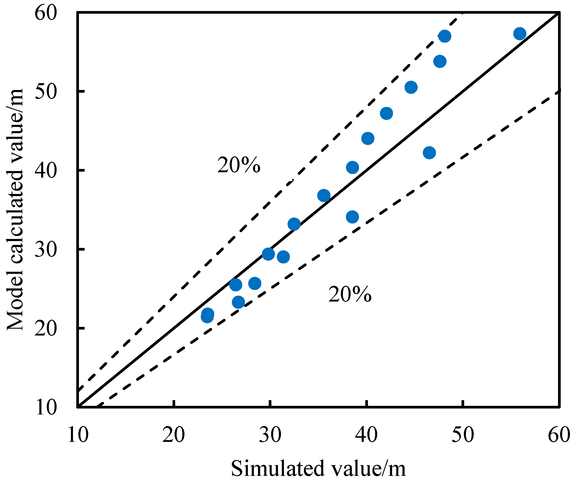
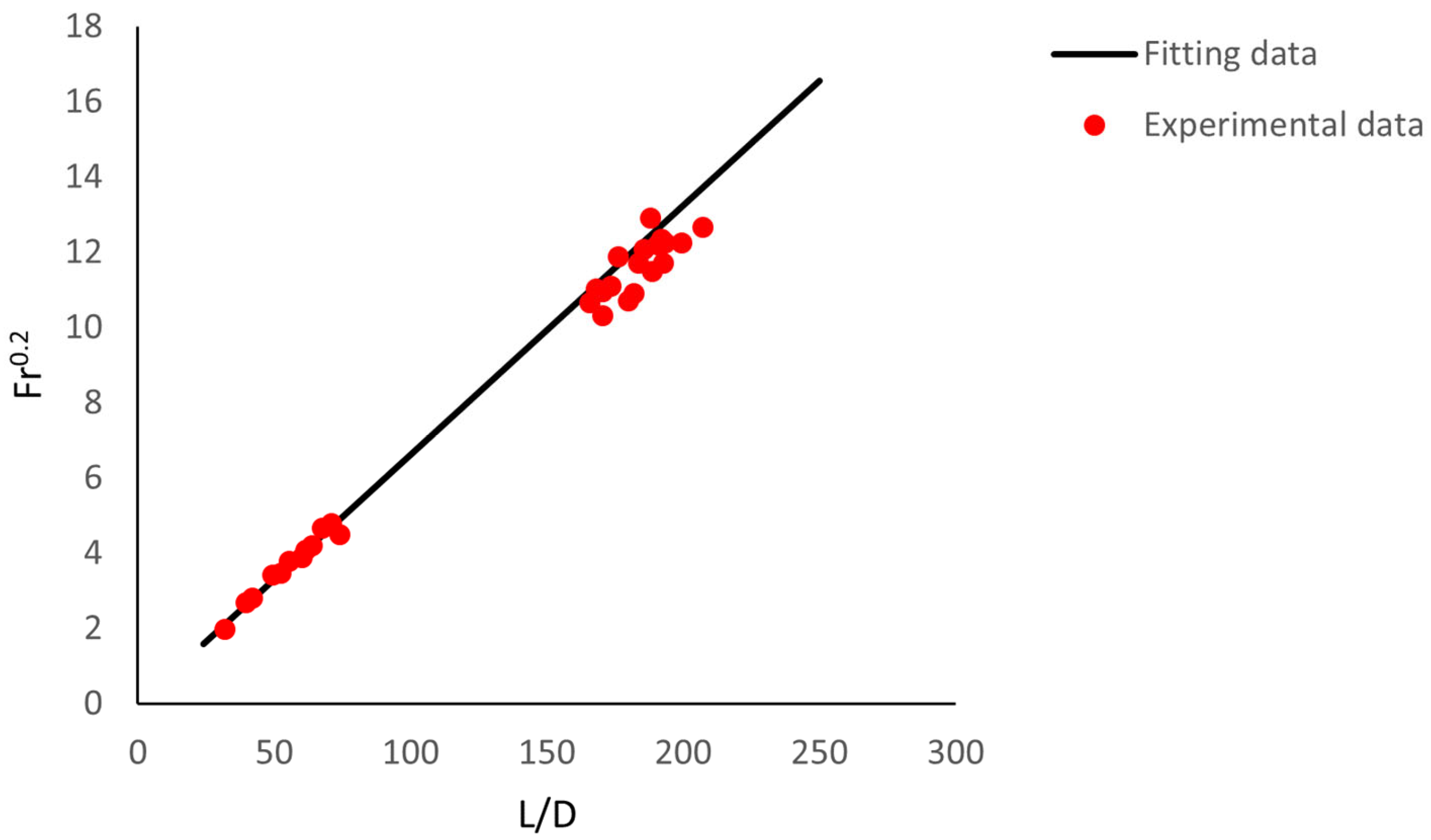
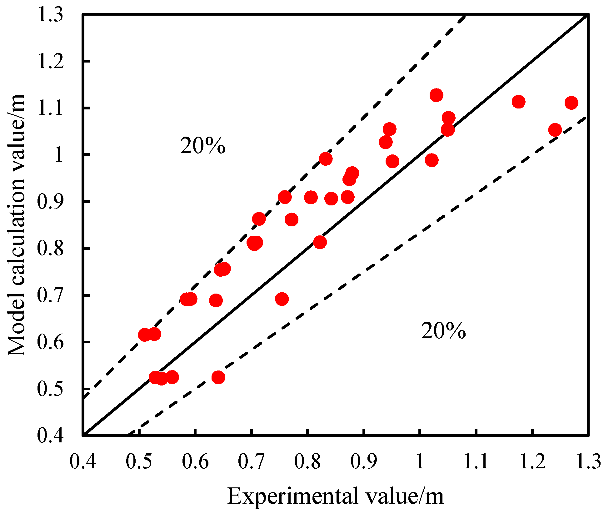
Prediction method for gas flow rate at the wellhead based on jet flame height

According to global research on jet flames [5,7,21], the dimensionless flame length of a jet flame is related to its Froude number. Therefore, with the calculation of the Froude number of methane gas and fitting of the simulation data, as shown in Figure 23, the mathematical relationship between the dimensionless flame height and Froude number is obtained as

$$\frac{L}{d}=15.1F{r}^{0.2}$$

(17)

$$Fr={(u^2/gL)}^{0.5}$$

(18)

Figure 24 shows the error between the experimentally obtained flame height and that calculated using Equation (13). The maximum, minimum, and average errors were 20.54%, 1.11%, and 11.28%, respectively.

Figure 25 shows the error between the simulated flame height and that calculated using Equation (13). The maximum, minimum, and average errors were 18.41%, 1.42%, and 8.37%, respectively.

The mathematical expression for predicting the gas flow rate at the wellhead using the flame height is

$$Q=\frac{L^{2.5}{g}^{0.5}\pi {\rho }_{\mathrm{a}}}{3544}$$

(19)

where ρ_a is the gas density at the wellhead, in kg·m⁻³.

(2)

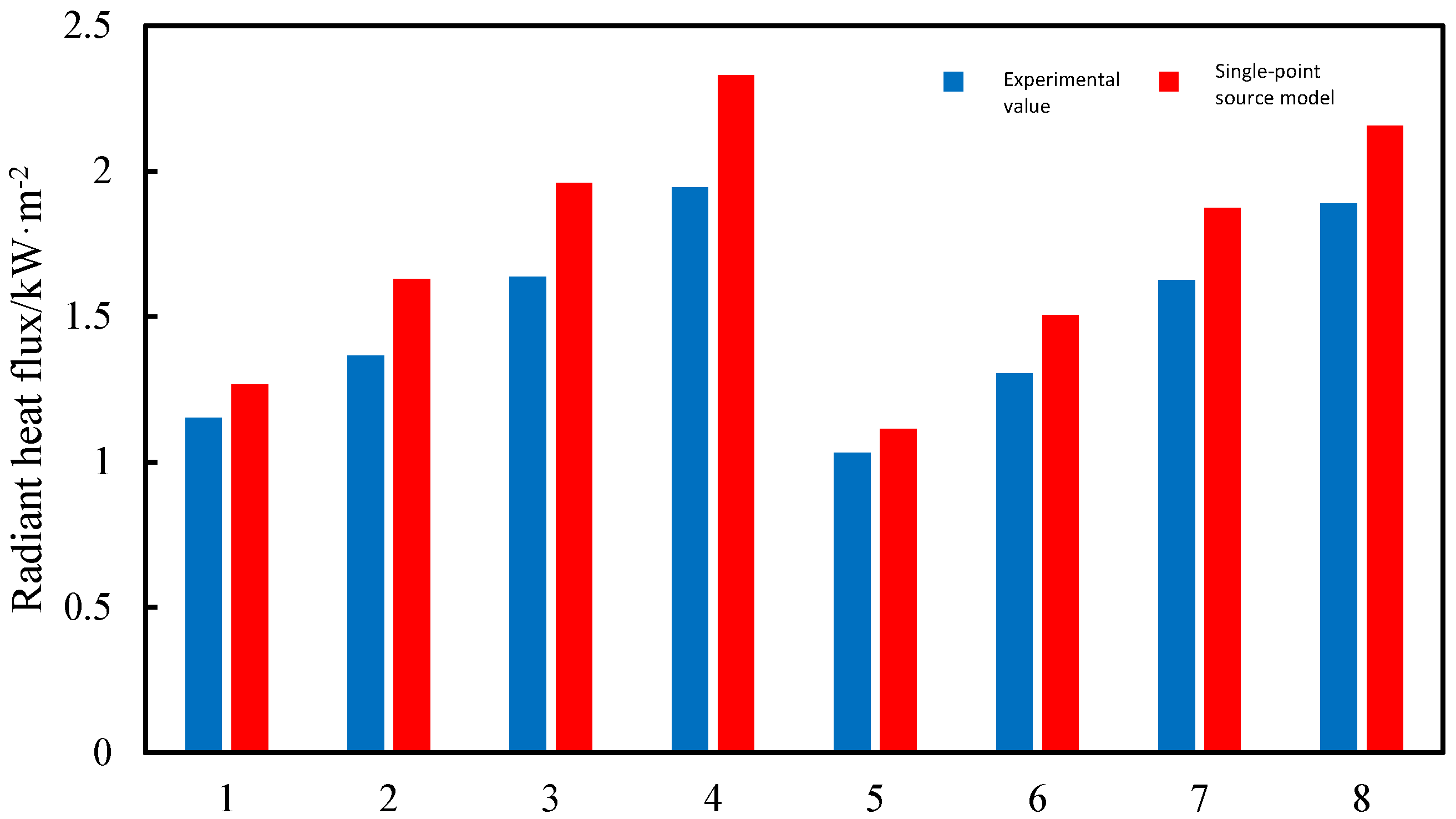
Prediction method for gas flow rate at the wellhead based on the thermal radiation intensity of the flame

The thermal radiation intensity of the blowout jet flame is proportional to the gas flow rate at the wellhead. Currently, the commonly used thermal radiation intensity calculation models, such as the single-point source model, are convenient and suitable for far-field flame thermal radiation research. Therefore, the single-point source model was chosen to explore the relationship between the gas flow rate at the wellhead and the thermal radiation intensity. The radiation calculation method for the single-point source model [6] is expressed as

$$q^{″}=\frac{\lambda X_{\mathrm{g}}Q△H}{4\pi R_{\mathrm{T}}^2}$$

(20)

where λ is atmospheric transmittance, in which λ = 1; X_g is the radiative heat fraction, in which X_g = 0.2; ∆H is the methane combustion heat value, in which ∆H = 52 × 10³ kJ·kg⁻¹; Q is the mass flow rate, in kg·s⁻¹; and R_T is the distance from the target object to the point source, in m.

The mathematical expression for predicting the gas flow rate at the wellhead using the thermal radiation intensity of the flame is

$$Q=\frac{4q^{″}\pi R_{\mathrm{T}}^2}{\lambda X_{\mathrm{g}}△H}$$

(21)

where q″ is the radiant heat flux, in kW·m⁻².

Figure 26 shows that the average error between the thermal radiation intensity of the jet flame calculated by the single-point source model and the experimental values is 15.17%.

(3)

Optimal prediction method for blowout gas volume

Based on the experimental data, the two methods for predicting the blowout gas volume were compared.

Table 2. Two types of well blowout gas volume prediction, with well blowout gas volume error table. Error table for predicting well jet volume of two types of wells.

Experimental Gas Volume/g·s−1	Gas Volume Predicted Based on Radiation/g·s−1	Error	Based on Flame Height Prediction of Gas Volume/g·s−1	Error
0.103	0.109	6.1%	0.115	11.9%
0.206	0.180	12.7%	0.218	5.6%
0.309	0.264	14.6%	0.276	10.9%
0.412	0.332	19.4%	0.378	8.4%
0.515	0.435	15.5%	0.612	18.7%
0.618	0.527	14.8%	0.556	10.2%
0.722	0.667	7.5%	0.661	8.4%
0.825	0.770	6.6%	0.777	5.8%
0.928	0.879	5.3%	0.897	3.3%
0.103	0.114	10.1%	0.120	16.9%
0.206	0.184	10.5%	0.222	7.7%
0.309	0.235	24.1%	0.302	2.4%
mean error		13.5%		7.75%

presents the inferred methane gas volumes using partial experimental data. A comparison of the predicted values from the two methods with the actual experimental values revealed that predicting the blowout gas volume based on the jet flame height yielded a higher accuracy, with an average error of 7.75%. This was because the single-point source model is a function of the gas velocity and distance between the target object and flame point source. The distance between the target object and flame point source is related to the flame height. Therefore, predicting the blowout gas volume using radiation intensity and flame height yields lower accuracy than when directly using the jet flame height to calculate the blowout gas volume. As a result, this study determined that the prediction method for blowout gas volume was based on the jet flame height.

5. Conclusions

This study focused on blowout jet fire accidents and investigated the morphology and combustion characteristics of blowout jet flames under different conditions through a combination of experimental and numerical simulation methods. From the experimental and simulation results, a prediction method for wellhead gas flow based on the blowout jet flame height was proposed, providing a scientific basis for emergency rescue operations in blowout fire accidents. The following conclusions and recommendations were drawn:

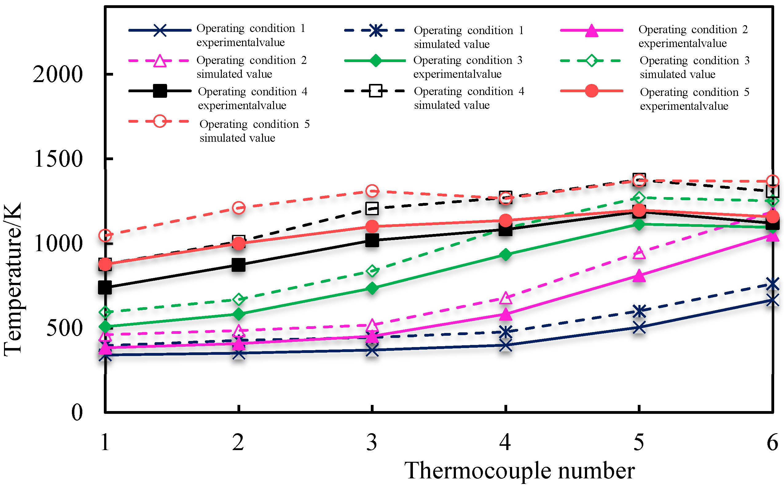
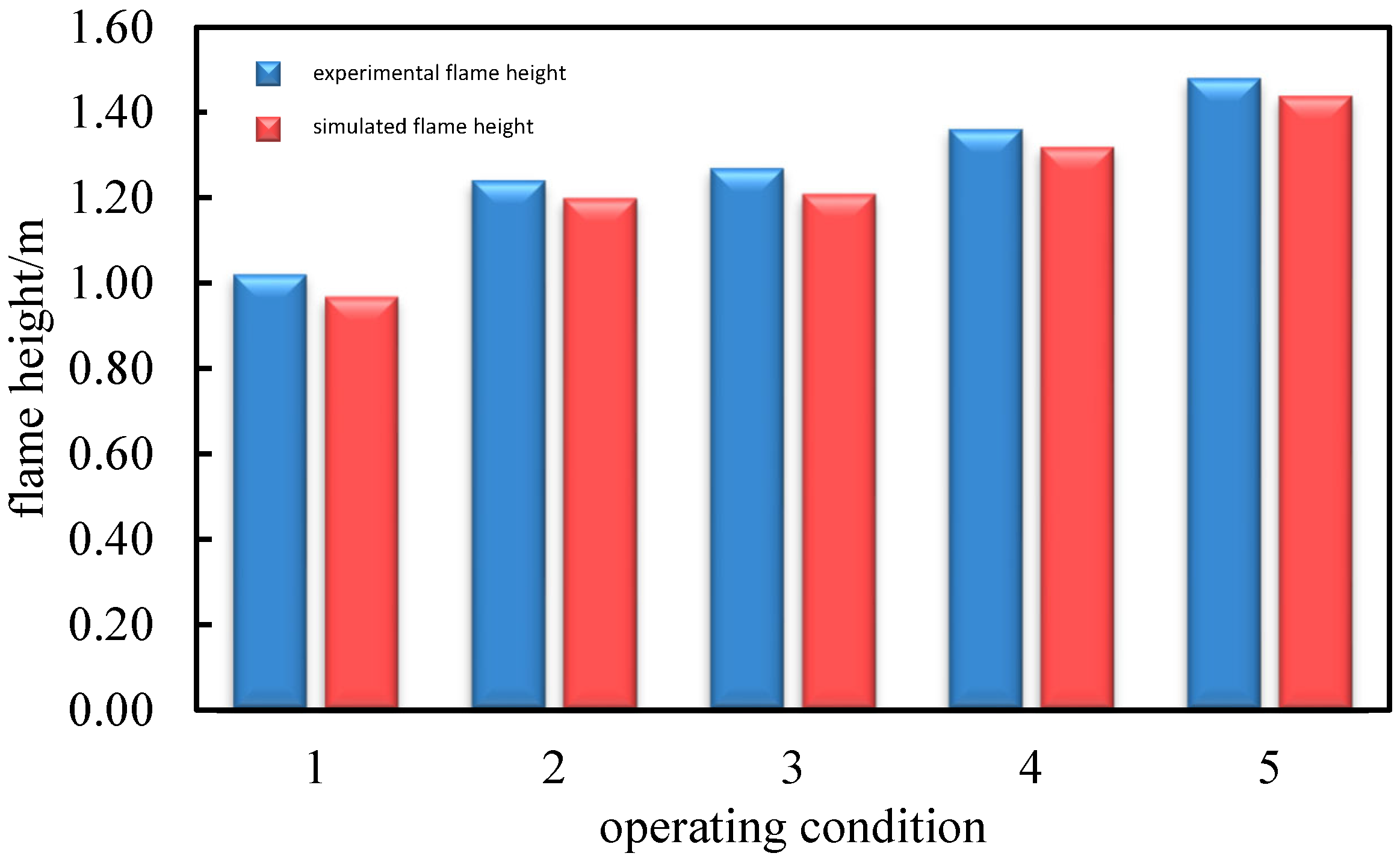
• Based on the characteristics of multicomponent gas and the turbulent state at the wellhead flame, a mathematical model that includes component transport and turbulent equations was established. Considering the under-expanded jet flow at the nozzle, a “virtual nozzle” was proposed to simplify the complex flow. Accordingly, a computational model of the blowout jet flame was established using FLUENT software 2021r2. The accuracy of the blowout jet flame calculation model was verified with experimental data, where errors for the simulated flame height, temperature, and thermal radiation were 8.91%, 16.94%, and 9.54%, respectively.
• A comparative analysis of the results obtained under different wind speeds, blowout gas volumes, and wellhead diameters revealed the effects of various external factors on the thermal radiation range of blowout jet fire accidents and the variation law of flame morphology. The jet flame height and thermal radiation intensity were positively correlated with the blowout gas volume, and the maximum temperature of the blowout jet flame was independent of the blowout gas volume. The wellhead diameter had little effect on the shape of the blowout jet flame of high-yield gas wells, where all were slender and elongated; under the same conditions, the longer the wellhead diameter, the higher was the flame height.
• Two prediction methods for blowout gas volume were proposed: an empirical formula based on flame height and an analytical model based on flame radiation. A comparison of the errors of the two methods in experimental data calculations revealed that the error for predicting the blowout gas volume using the blowout jet flame height was 7.75%, which proved simpler and more accurate than when predicting the blowout gas volume using flame radiation.

References

- Suris, A.L.; Flankin, E.V.; Shorin, S.N. Length of free diffusion flames. Combust. Explos. Shock Waves 1978, 13, 459–462. [Google Scholar] [CrossRef]
- Røkke, N.A.; Hustad, J.E.; Sønju, O.K. A study of partially premixed unconfined propane flames. Combust. Flame 1994, 97, 88–106. [Google Scholar] [CrossRef]
- Costa, M.; Parente, C.; Santos, A. Nitrogen oxides emissions from buoyancy and momentum controlled turbulent methane jet diffusion flames. Exp. Therm. Fluid Sci. 2004, 28, 729–734. [Google Scholar] [CrossRef]
- Santos, A.; Costa, M. Reexamination of the scaling laws for NOx emissions from hydrocarbon turbulent jet diffusion flames. Combust. Flame 2005, 142, 160–169. [Google Scholar] [CrossRef]
- Kiran, D.Y.; Mishra, D.P. Experimental studies of flame stability and emission characteristics of simple LPG jet diffusion flame. Fuel 2007, 86, 1545–1551. [Google Scholar] [CrossRef]
- Palacios, A.; Muñoz, M.; Casal, J. Jet fires: An experimental study of the main geometrical features of the flame in subsonic and sonic regimes. AIChE J. 2009, 55, 256–263. [Google Scholar] [CrossRef]
- Zhou, K.; Liu, J.; Jiang, J. Prediction of radiant heat flux from horizontal propane jet fire. Appl. Therm. Eng. 2016, 106, 634–639. [Google Scholar] [CrossRef]
- Gopalaswami, N.; Liu, Y.; Laboureur, D.M.; Zhang, B.; Mannan, M.S. Experimental study on propane jet fire hazards: Comparison of main geometrical features with empirical models. J. Loss Prev. Process Ind. 2016, 41, 365–375. [Google Scholar] [CrossRef]
- Stfnju, O.K.; Hustadf, J. An Experimental Study of Turbulent Jet Diffusion Flames; British Maritime Technology: London, UK, 1983. [Google Scholar]
- Haas, L. Reprints available directly from the publisher Photocopying permitted by license only. Rev. Educ. Pedagog. Cult. Stud. 1995, 17, 1–6. [Google Scholar] [CrossRef]
- Bagster, D.F.; Schubach, S.A. The prediction of jet-fire dimensions. J. Loss Prev. Process Ind. 1996, 9, 241–245. [Google Scholar] [CrossRef]
- Imamura, T.; Hamada, S.; Mogi, T.; Wada, Y.; Horiguchi, S.; Miyake, A.; Ogawa, T. Experimental investigation on the thermal properties of hydrogen jet flame and hot currents in the downstream region. Int. J. Hydrogen Energy 2008, 33, 3426–3435. [Google Scholar] [CrossRef]
- Mogi, T.; Horiguchi, S. Experimental study on the hazards of high-pressure hydrogen jet diffusion flames. J. Loss Prev. Process Ind. 2009, 22, 45–51. [Google Scholar] [CrossRef]
- Palacios, A.; Casal, J. Assessment of the shape of vertical jet fires. Fuel 2011, 90, 824–833. [Google Scholar] [CrossRef]
- Bo, Z.; Shuang, L.; Pengcheng, W. Comparative analysis of the influence range and model of thermal radiation caused by blowout and jet fire. China Saf. Prod. Sci. Technol. 2022, 18, 139–144. [Google Scholar]
- Qihua, W.; Zhanwen, L.; Zhijiu, A. Simulation study on uncontrolled blowout and jet fire under different gas production rates. Saf. Environ. Eng. 2009, 16, 103–107. [Google Scholar]
- Mashhadimoslem, H.; Ghaemi, A.; Palacios, A.; Behroozi, A.H. A new method for comparison thermal radiation on large-scale hydrogen and propane jet fires based on experimental and computational studies. Fuel 2020, 282, 118864. [Google Scholar] [CrossRef]
- Li, G. Numerical simulation study on combustion characteristics of mixed fuels containing CO. Ph.D. Thesis, Beijing University of Technology, Beijing, China, 2010. [Google Scholar]
- Mashhadimoslem, H.; Ghaemi, A.; Behroozi, A.H.; Palacios, A. A New simplified calculation model of geometric thermal features of a vertical propane jet fire based on experimental and computational studies. Process Saf. Environ. Prot. 2020, 135, 301–314. [Google Scholar] [CrossRef]
- Kim, Y.S.; Jeon, J.; Song, C.H.; Kim, S.J. Improved prediction model for H2/CO combustion risk using a calculated non-adiabatic flame temperature model. Nucl. Eng. Technol. 2020, 52, 2836–2846. [Google Scholar] [CrossRef]
- Lowesmith, B.J.; Hankinson, G.; Acton, M.R.; Chamberlain, G. An Overview of the Nature of Hydrocarbon Jet Fire Hazards in the Oil and Gas Industry and a Simplified Approach to Assessing the Hazards. Process Saf. Environ. Prot. 2007, 85, 207–220. [Google Scholar] [CrossRef]