Data-Driven Method for Vacuum Prediction in the Underwater Pump of a Cutter Suction Dredger

Abstract

Vacuum is an important parameter in cutter suction dredging operations because the equipment is underwater and can easily fail. It is necessary to analyze other parameters related to the vacuum to make real-time predictions about it, which can improve the construction efficiency of the dredger under abnormal working conditions. In this paper, a data-driven method for predicting the vacuum of the underwater pump of the cutter suction dredger (CSD) is proposed with the help of big data, machine learning, data mining, and other technologies, and based on the historical data of “Hua An Long” CSD. The method eliminates anomalous data, standardizes the data set, and then relies on theory and engineering experience to achieve feature extraction using the Spearman correlation coefficient. Then, six machine learning methods were employed in this study to train and predict the data set, namely, lasso regression (lasso), elastic network (Enet), gradient boosting decision tree (including traditional GBDT, extreme gradient boosting (XGBoost), light gradient boosting machine (LightGBM)), and stacking. The comparison of the indicators obtained through multiple rounds of feature number iteration shows that the LightGBM model has high prediction accuracy, a good running time, and a generalization ability. Therefore, the methodological framework proposed in this paper can help to improve the efficiency of underwater pumps and issue timely warnings in abnormal working conditions.

1. Introduction

Dredging is now of increasing importance in the field of water transportation and integrated environmental management. CSDs have become the preferred choice for dredging programs in many ports due to their superior efficiency, simplicity of operation, and cost-effectiveness. Underwater pumps, as the power equipment for transferring dredged sediments, are the core equipment in the operation process of a CSD. Therefore, whether the underwater pump can work normally is related to whether the dredger can continue to operate, and improving the reliability of an underwater pump with a complex structure is the key to ensuring uninterrupted and efficient operation. A CSD underwater pump used in construction is not always within its normal operating range, as the actual underwater pump vacuum may be higher than the theoretical value. The suction pipe inlet may be clogged or the pipeline mud concentration may be too high. If the CSD construction parameters are not adjusted in a timely manner, this may lead to the suction pipe being blocked, greatly reducing the construction efficiency of the CSD. Therefore, it is one of the important directions in the research field of dredging to keep the underwater pump in the normal working interval as reliably as possible, in order to ensure the safe operation of the equipment and improve the operation efficiency at the same time.

Due to the fact that a change in the underwater pump’s working state will lead to a change in its vacuum, vacuum is an important parameter to consider when judging the working state of an underwater pump. The underwater pump sliding into an abnormal working area will affect production efficiency and may also damage the equipment and sensors. It must therefore be ensured that operators master the real-time working state of the underwater pump to make the corresponding judgment in a timely manner. The operating environment of the dredger is inherently complex and affected by many factors. In each construction period, soil quality changes, bench feed, seawater, geotechnical concentration, the equipment itself, and other factors, including poor working conditions, may lead to the failure of the vacuum sensor, resulting in an inability to accurately measure the underwater pump vacuum. Therefore, predicting the vacuum of the underwater pump in real time is crucial to the safe operation of the dredger.

With the development of artificial intelligence, researchers have applied various techniques and methods to solve the problems of sensor failure, sensor perception enhancement, and parameter prediction. Wang et al. [1] proposed a data mining method of model stacking generalization to predict the productivity of a suction dredger, which superimposed five machine learning models, and the results show that the performance of the stacked generalized model outperformed that of other studied algorithms. Bai et al. [2] used machine learning algorithms, including XGBoost, to predict the productivity of CSDs with more than 90% accuracy, outperforming traditional methods. Specifically, the digital twin-driven virtual sensor approach, which can solve the problem of sudden sensor failure, has recently become a popular research direction. Digital twins can improve the accuracy and efficiency of data prediction for complex equipment operating in harsh environments, especially in prognostics and health management (PHM). Li et al. [3] introduced a digital twin-driven virtual sensor (DTDVS) that predicts the state of a dredger, diagnoses the construction behavior, and provides accurate warnings of failure conditions by analyzing the residuals between the physical and virtual sensors. Han et al. [4] addressed the hysteresis effect in the design of a CSD and then proposed a method to analyze and predict the mud concentration utilizing machine learning and a hybrid integration strategy, which is modified to achieve short-term prediction with the help of other real-time signals. Booyse et al. [5] proposed a deep digital twin (DDT) to address the problem of over-reliance on historical data in detecting faults and tracking degradation under different conditions. As dredging has become smarter, various artificial intelligence techniques, machine learning, and deep learning methods have been widely used for productivity prediction.

The increasing maturity of big data prediction methods has made it possible to predict the vacuum level of the underwater pump condition of a CSD using data-driven methods. In this paper, such a method is proposed and evaluated in comparison with five machine learning and deep learning methods. The proposed method helps the operator to sense the failure of the underwater pump in time and return the underwater pump to the operational state by adjusting the parameters of the associated features.

This paper is organized as follows. Section 2 describes the methodology and work of data preprocessing. Section 3 proposes a feature term selection method based on a combination of theoretical reality basis and Spearman correlation analysis. Section 4 describes the training and selection of prediction models based on a comparative evaluation of multiple computational models. Section 5 discusses the results of the model training and makes selection judgments based on the evaluation results. Section 6 describes a generalization ability assessment based on the preferred model and presents the models and engineering application methods applicable to vacuum prediction. Section 7 presents the conclusion of the paper.

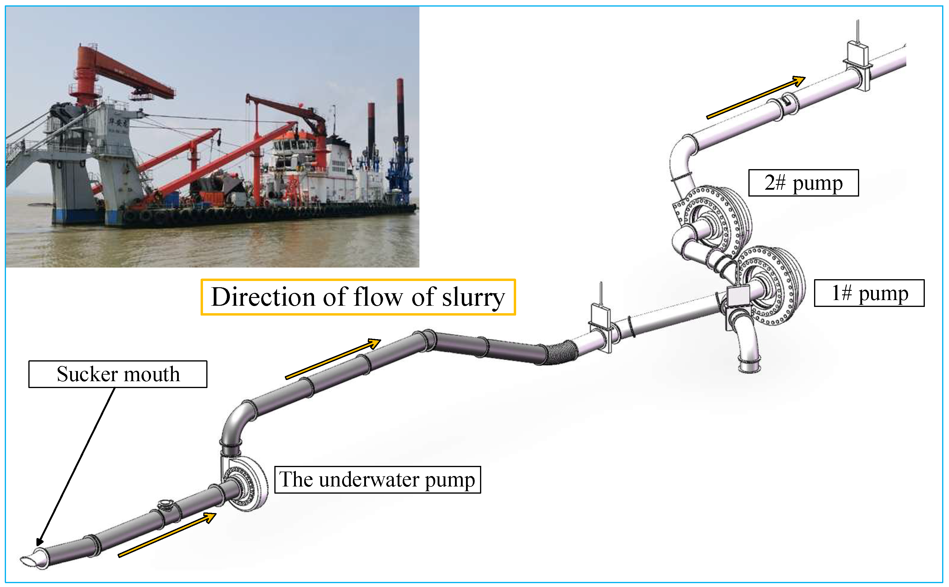
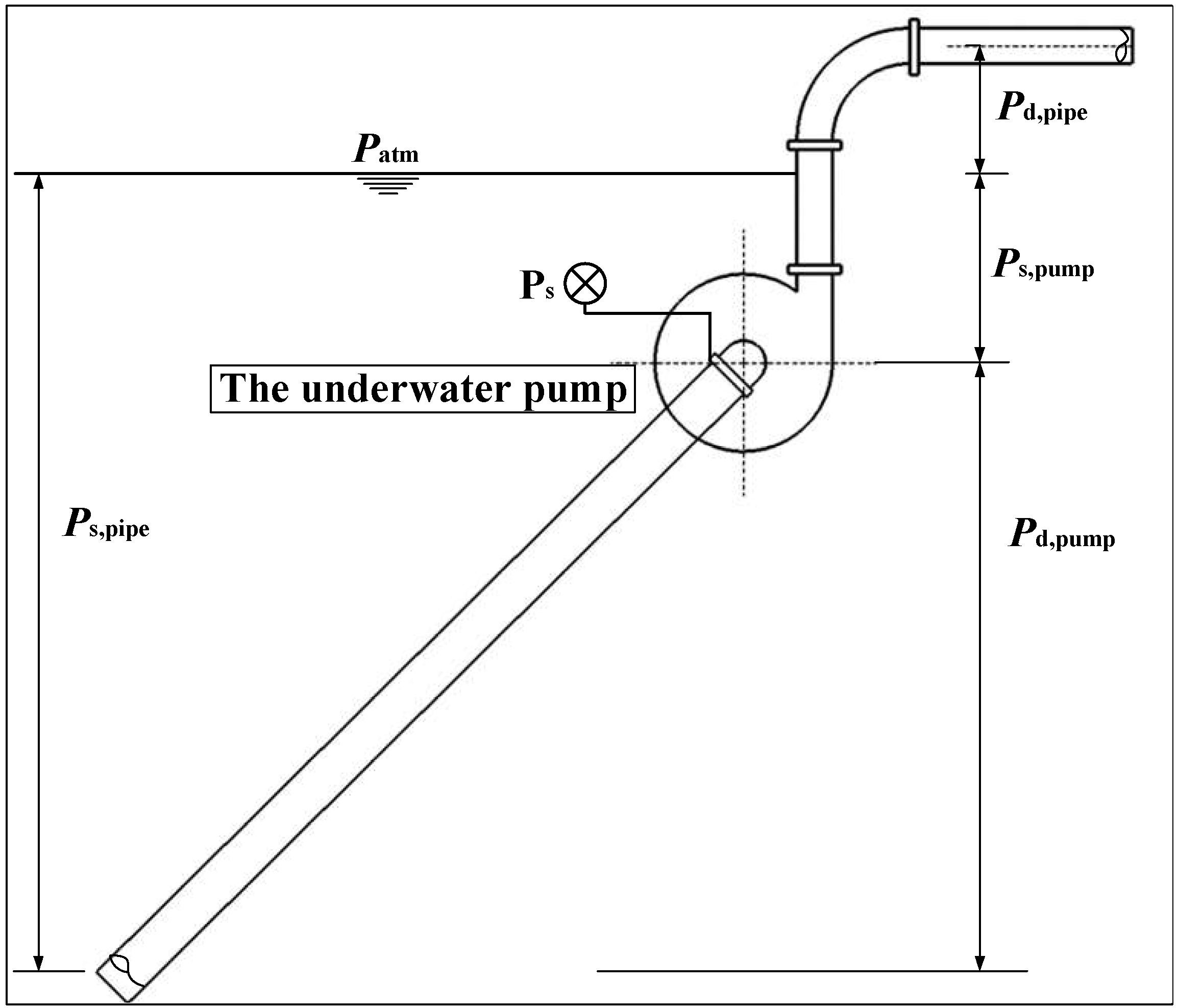
2. Research Object and Methodology

2.1. Construction Process for CSDs

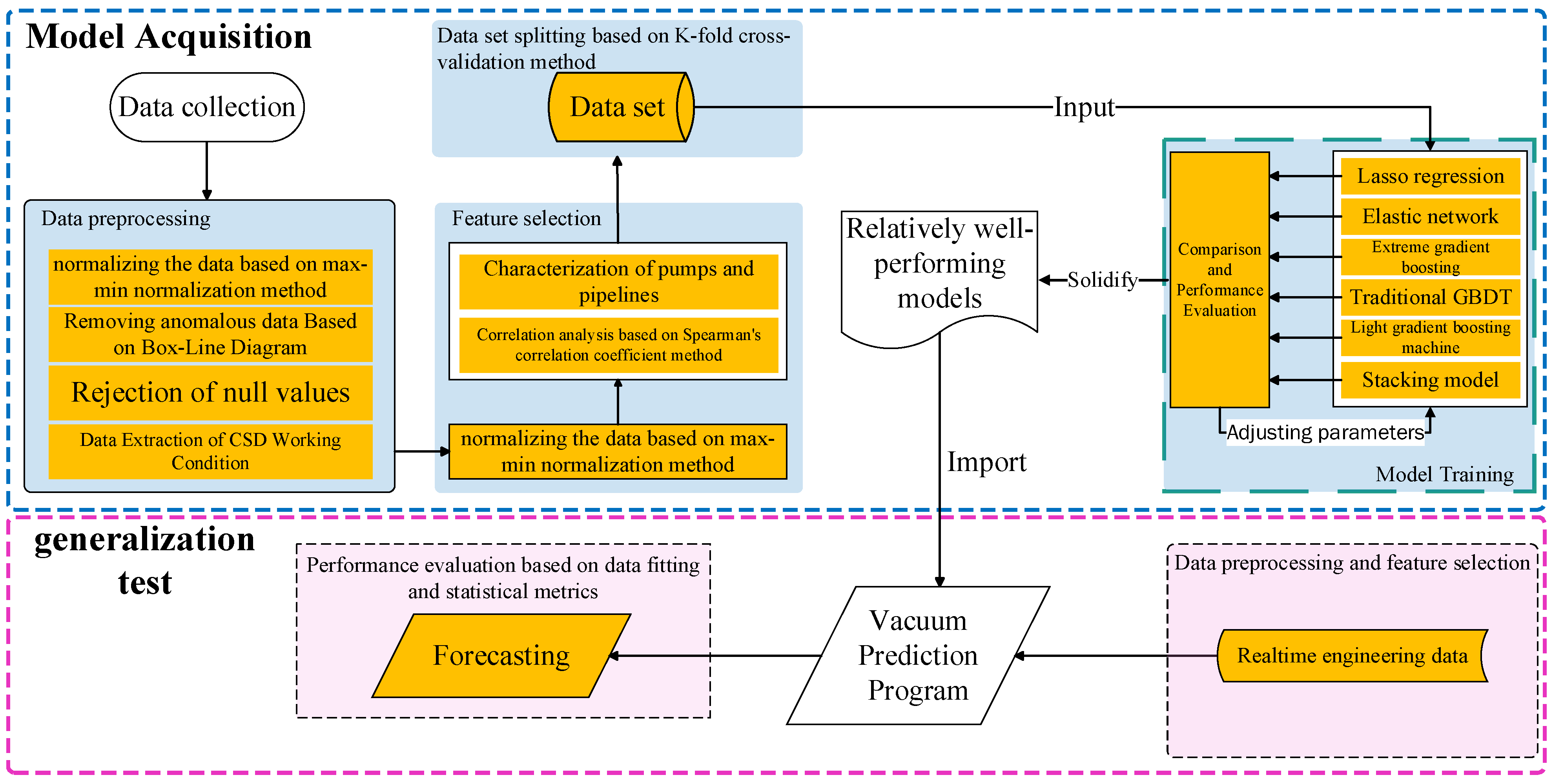
The research work of this paper is based on existing engineering data, which were collected by suction dredger as shown in Figure 1. During the work process, the CSD uses the underwater pump to collect the mud underwater and the mud is transported through the pipe to the target location; this work needs more than one pump to be complete, as shown in Figure 1. During the process, the underwater pump will produce negative pressure in front of the pump, causing the mud to enter the pipeline through the suction port. Due to the lifting effect of the 1# pump, the mud will then flow from the bottom to the water surface, and then the 2# pump will cause the mud to be transported to the target location.

In the pipeline system, the pump’s output power is matched with the pipeline characteristics, and is mainly affected by the inlet pressure, the flow rate of the slurry, and the resistance along the pipeline. The resistance is mainly affected by the density of the slurry itself and other factors. Independently from the pump, the output power, output pressure, and flow rate are interrelated, and the output pressure includes the vacuum before the pump and the head pressure behind the pump.

From the perspective of efficiency and relevance, the operator of a suction dredger in the construction process needs to ensure that the underwater pump works in the high-efficiency zone. Due to its ability to respond to a wide range of changes in the pumps and pipelines, the vacuum of the underwater pump is often used as an important parameter of analysis, in order to monitor and prevent siltation and vapor corrosion. The theoretical calculation model for vacuum in the underwater suction pipe of the CSD is shown in Figure 2, and the theoretical calculation formula is as follows:

$$Vacuum=P_{\mathrm{atm}}+{\mathit{\rho }}_{w}g1-{\mathit{\rho }}_{m}g(h_{s,pipe}-h_{s,pump})-{\mathit{\rho }}_{w}g{H}_{totloss,s}m-{\mathit{\rho }}_m{V}_s^2/2$$

(1)

where $P_{\mathrm{atm}}$ represents the atmospheric pressure, the suction mouth depth is $h_{s,pipe}$, $h_{s,pump}$ represents the mud pump depth, the suction line friction loss is $H_{totloss,s}$, and the flow velocity is $V_s$.

According to the results of the theoretical analysis, it can be said that the vacuum degree has a strong correlation with the feature terms. After further comprehensive consideration of the Spearman correlation coefficient, this study selected 56 parameters. They are the suction seal water pressure of the underwater pump, the suction seal water pressure of the 1# pump, the suction seal water pressure of the 2# pump, the shaft seal water pressure of the underwater pump, the shaft seal water pressure of the 1# pump, the shaft seal water pressure of the 2# pump, the speed of the 1# pump, the speed of the 2# pump, the speed of the underwater pump, velocity, density, the torque of the underwater pump, the motor speed of the underwater pump, the pressure of the hydraulic cylinder of the dolly, the pressure of the hydraulic cylinder of the steel pile, the pressure of the gate valve system, dolly travel, left traverse speed, right traverse speed, the rotational speed of the reamer, the discharge pressure of the 1# pump, the discharge pressure of the 2# pump, the discharge pressure of the underwater pump, Bridge Angle, the x-coordinate of GPS1, the y-coordinate of GPS1, the speed of GPS1, tide level, water density, trunnion draft, traverse speed, the x-coordinate of the reamer, the y-coordinate of the reamer, outlet flow rate, left traverse torque, reamer torque, concentration, volume, right traverse torque, left anchor winch speed, left anchor winch torque, right anchor winch speed, right anchor winch torque, left slewing winch torque, right slewing winch speed, right slewing winch torque, left slewing winch speed, bridge hoisting winch speed, bridge hoisting winch torque, bridge depth, reamer cutting angle, underwater pump power, sludge pump power, average concentration in pipeline, the height of the underwater pump, and suction pressure.

2.2. Methodology

The research presented in this paper was based on the existing construction data for a stranded suction dredger; by analyzing the characteristics of the impact of the underwater pump in the construction process, we aimed to determine the change rule for the vacuum degree of the underwater pump. Figure 3 demonstrates the process of the research presented in this paper. We began with the existing engineering data, and we eliminated the noise in the data preprocessing stage. Heat map visualization of the feature correlation was achieved, helping to reduce the dimensionality of the data set. In this study, six different machine learning models were selected using the characteristics of the construction data, with the aim of selecting suitable models through several rounds of training and parameter tuning. Finally, this study carried out a generalization ability assessment on the selected models using additional datasets to evaluate the engineering applicability of the models selected using this method.

3. Data Preprocessing

Considering the poor quality of the raw data, duplicates, redundancies, and useless data needed to be removed before data processing. In addressing the problem of possible missing data in the provided data set and to obtain more accurate data for the feature items, the missing values needed to be processed. The original data were affected by the working environment of the equipment and other factors. There may have been distortions, and the extracted data also needed to be processed to ensure the authenticity and validity of the feature items. The original data had different scales, and their numerical differences may have affected the results of correlation analysis. Therefore, they could not be used directly as the formatting samples for constructing the model; they needed to be normalized in order to eliminate the influence of scales and value ranges between indicators.

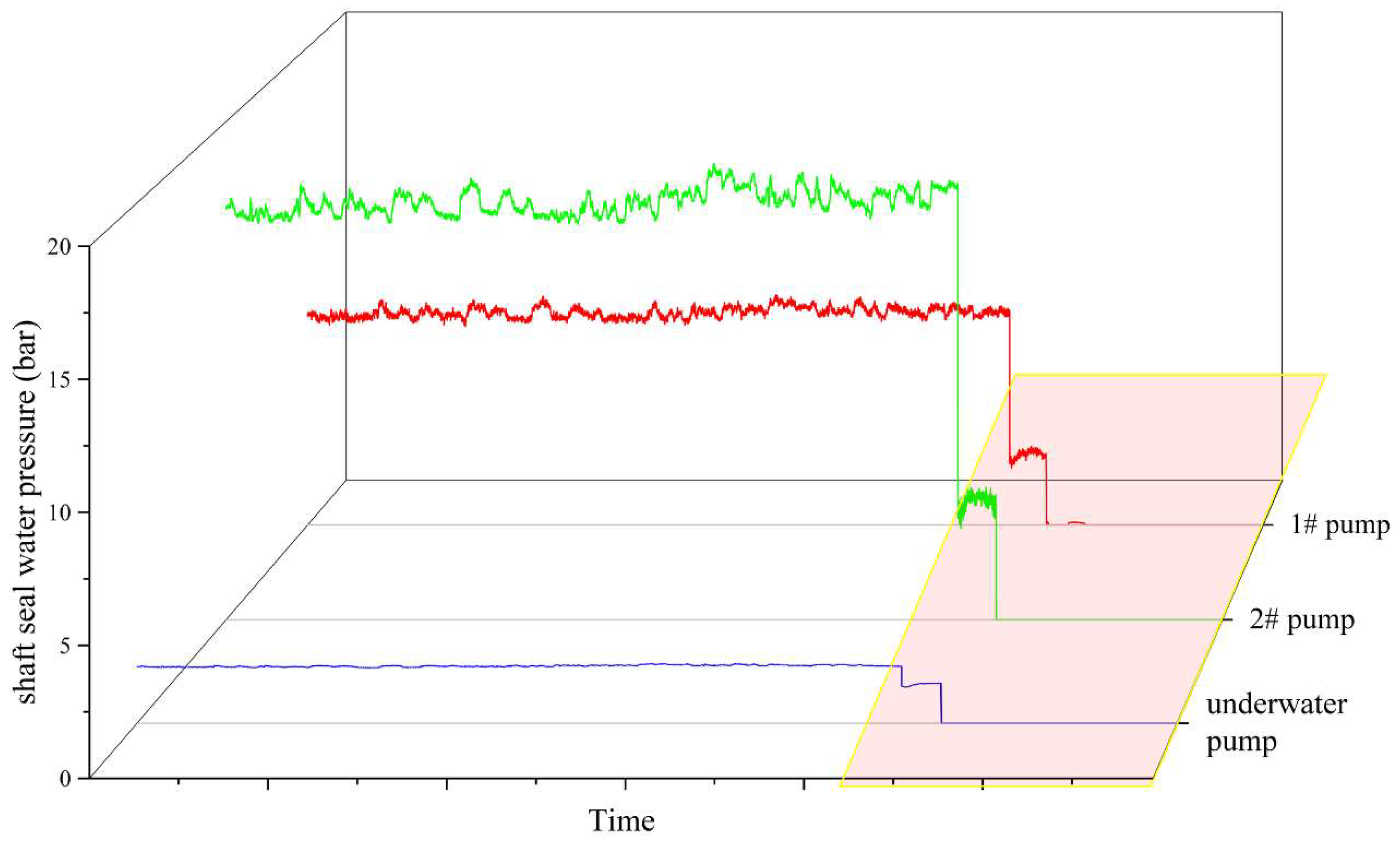
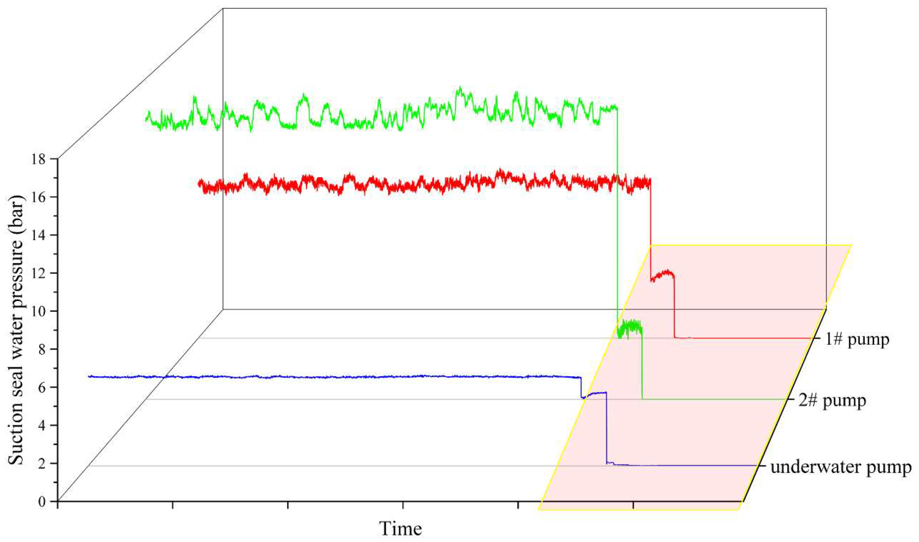
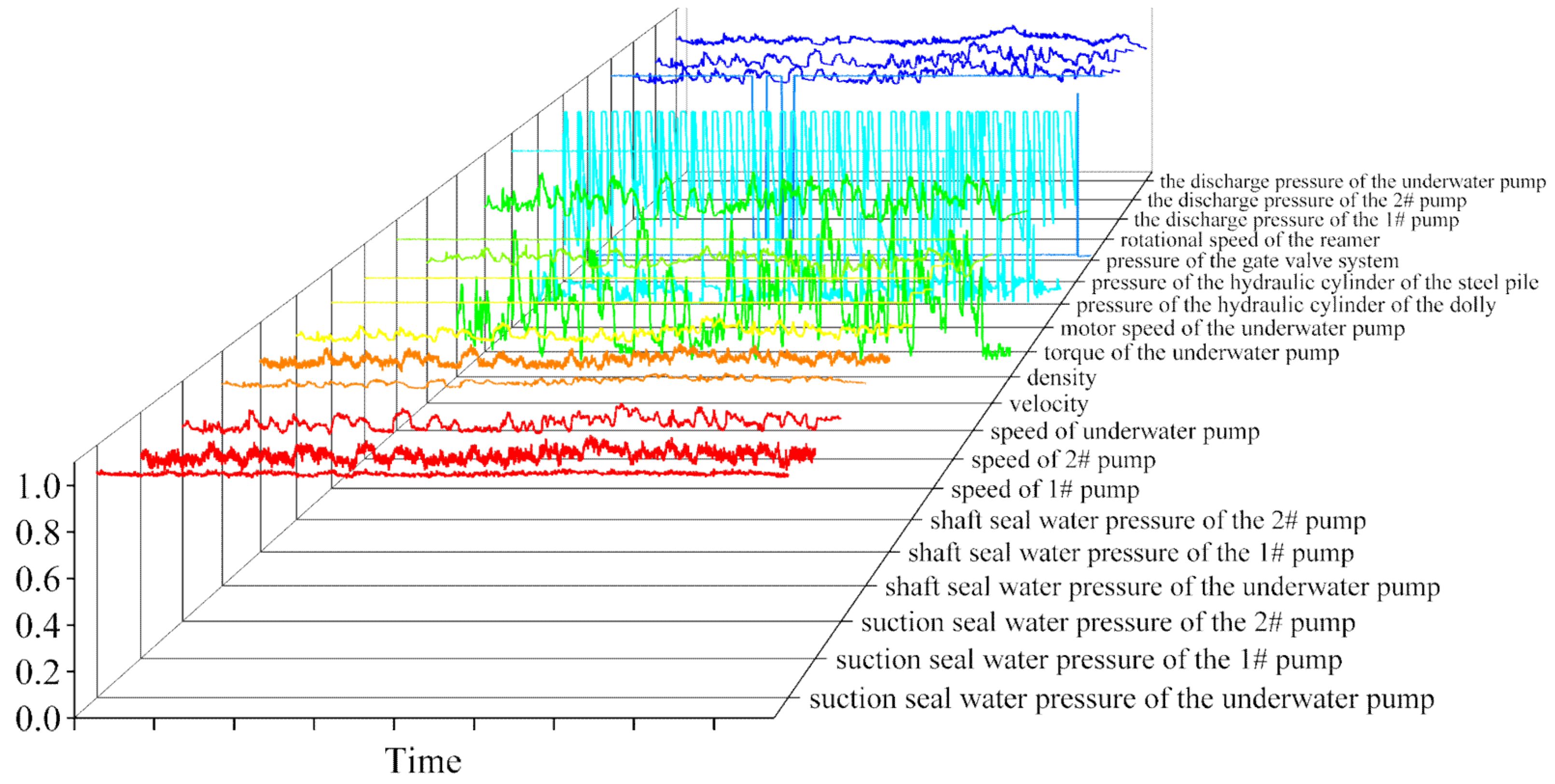
3.1. Data Observation and Extraction

The data studied in this paper are discrete data collected at three-second intervals, with a total of 63 characteristic parameters recorded, as shown in

Table 1. Example data set.

Serial Number	Time	Shaft Seal Water Pressure of the Underwater Pump (Bar)	Suction Seal Water Pressure of the Underwater Pump (Bar)	…	Height of the Underwater Pump (m)	Suction Pressure (Pa)	Vacuum (Bar)
1	2022-11-08 06:00:01	4.78	2.17	…	4.37	85,526.19	0.1559
2	2022-11-08 06:00:04	4.82	2.18	…	4.38	85,410.67	0.1570
3	2022-11-08 06:00:07	4.79	2.17	…	4.38	85,410.67	0.1570
4	2022-11-08 06:00:11	4.78	2.18	…	4.38	88,443.31	0.1271
…	…	…		…	…	…	…
5955	2022-11-08 11:59:54	0.02	0	…	−6.61	−33,717.80	1.3327
5956	2022-11-08 11:59:57	0.02	0	…	−6.62	−34,557.10	1.3410
5957	2022-11-08 12:00:00	0.02	0	…	−6.61	−34,791.47	1.3433

. The individual data are floating-point numbers in time order. The data set contains a number of feature items that are not related to the gibbet system and delivery piping of the gibbet vessel, and these extraneous quantities can be eliminated before importing. There are Chinese feature variable names, variable numbers, and times in the table, so attention should be paid to the type of data after data importing. The Chinese variable names should be stored as strings in the program and should be prevented from being garbled so that the features can be referenced at a later stage. The Spearman correlation coefficient method is based on random floating-point data feature extraction, and one does not need to pay attention to the distance between the samples in order to maintain the normal order of the data to meet the implementation of the correlation coefficient analysis. Therefore, in the preparation of this program, before importing, the data will be placed in chronological order. Rearranging the time item in the subsequent modeling process no longer has a role. Therefore, the time term can be eliminated during the data import process.

The data analysis must be based on the data generated in the actual production process of the dredger; that is to say, it is necessary to filter out the abnormal data in the non-operational stage, which can significantly improve the accuracy of the results. Establishing the state of the ship’s operation process should be a stable basis for judgment. Figure 4, Figure 5 and Figure 6 illustrate part of the key data of the three mud pumps in the ship’s operation process under three parameter changes. The highlighted part of the data for each parameter illustrates a sudden change in the situation where the parameter has stabilized in a smaller value. This shows that the mud pump may be in an idle state, which means that the ship is very probably in a non-operational state. However, even if the pump is not idling, the data should be processed in the data cleaning phase to be on the safe side, considering that each data item has a sudden change and stabilizes at a relatively small value.

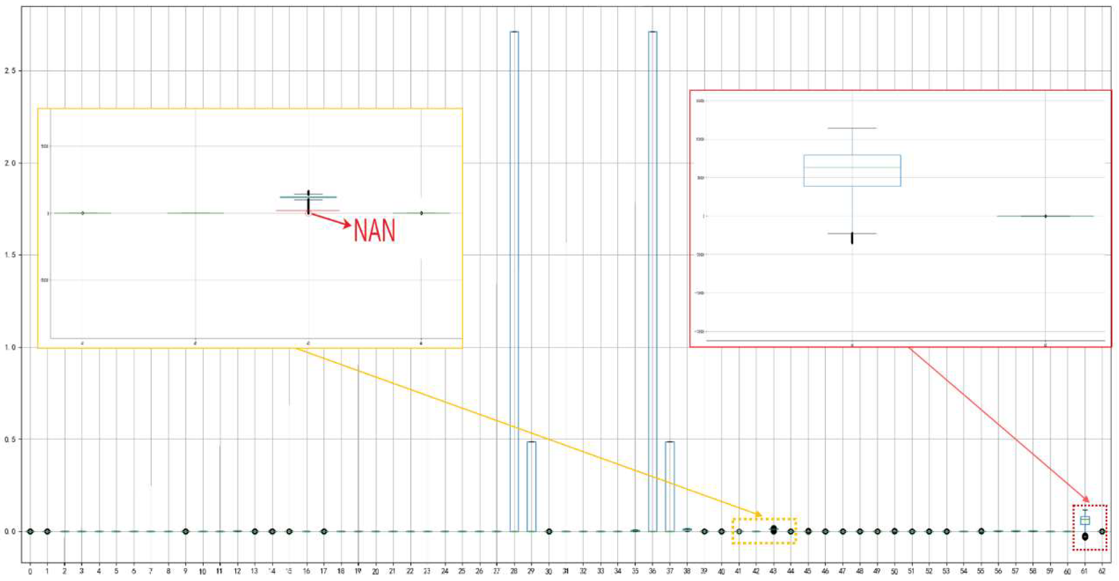
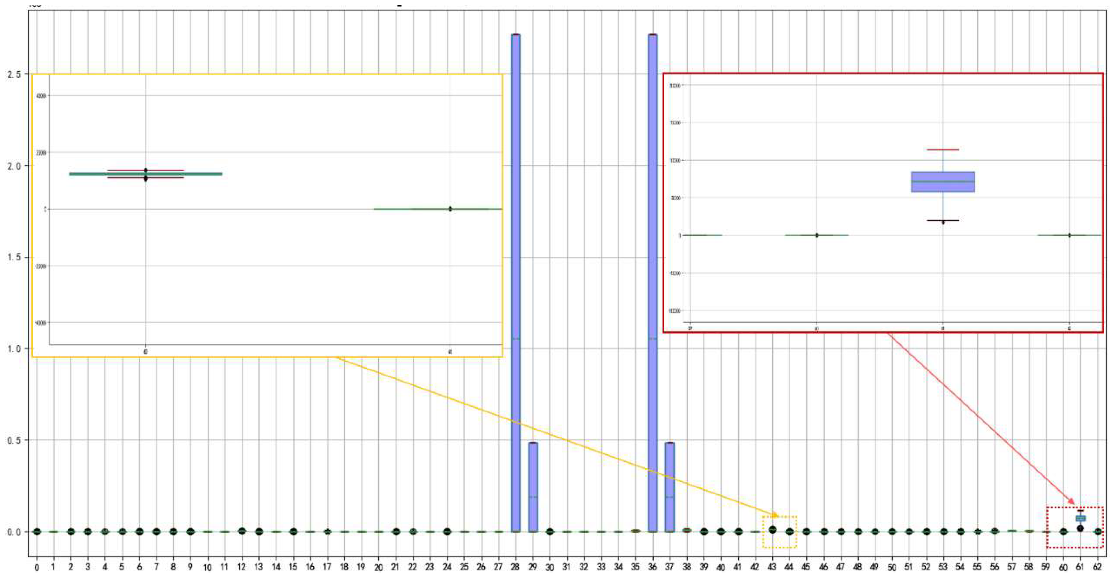
3.2. Handling of Missing Values and Outliers

There may be special reasons why values are missing, such as abnormalities in the data collection equipment, which may lead to abnormalities in other items of data at the same moment. Missing values represent a small percentage compared to the large original data set and have little impact on the problem, so it was decided that the whole group should be discarded. In this study, missing values were monitored using algorithmic identification, and then data sets with missing values were discarded using algorithmic tools.

The model is usually an expression of the data structure of the overall sample, which usually captures its general properties. Some properties behave completely inconsistently with the overall sample, that is, they exist in a generation mechanism that is completely inconsistent with the overall sample. This leads to the generation of a model that does not provide a good representation of the overall sample, and thus the prediction will be inaccurate. During construction, the reliability of the sensors may cause one or more parameters to be missing from a single set of data, and such anomalies can have a significant impact on the results of the data analysis. This is why we chose not to assign values at a later stage, which would have introduced more randomness. The original data set was recorded as discrete floating-point data. We chose to convert the data into floating-point numbers and then delete the data items with null values with the help of the dropna function in the data module. The box-and-line diagram method arranges the data according to size, and then takes the median of each parameter as the core, according to the size of the values on both sides of the median in the order of the equidistributional of the limit. It then obtains the limit difference, through the introduction of coefficient terms to control the outlier cutoff point, which shows that the applicability of a variety of distributional data is good. The original data set, shown in Figure 7, is analyzed with the help of the box-and-line diagram method, and a box-and-line diagram, shown in Figure 8, is obtained. However, it can be seen that there still are some anomalies. In this paper, taking into account the existence of large data fluctuations and the inability to determine whether this represents anomalous mutation or not, the data outside the outer limit are excluded. At the same time, the upper and lower limits of the degree of stringency are appropriately reduced, in order to retain enough data for model training and testing. This leads to a small amount of features still outside the outer limit, but the impact of these data is relatively small overall, and thus they will not be excluded here.

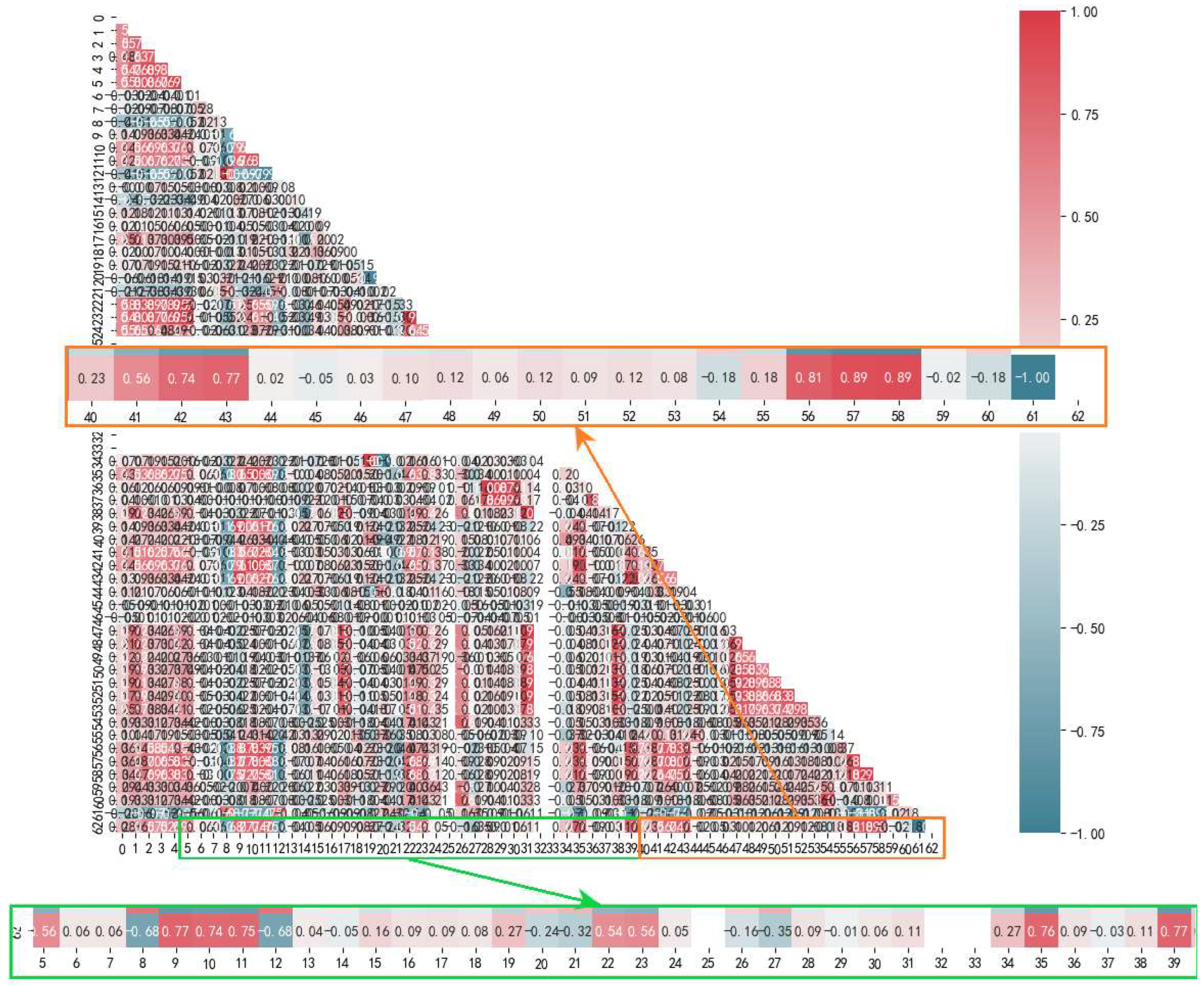
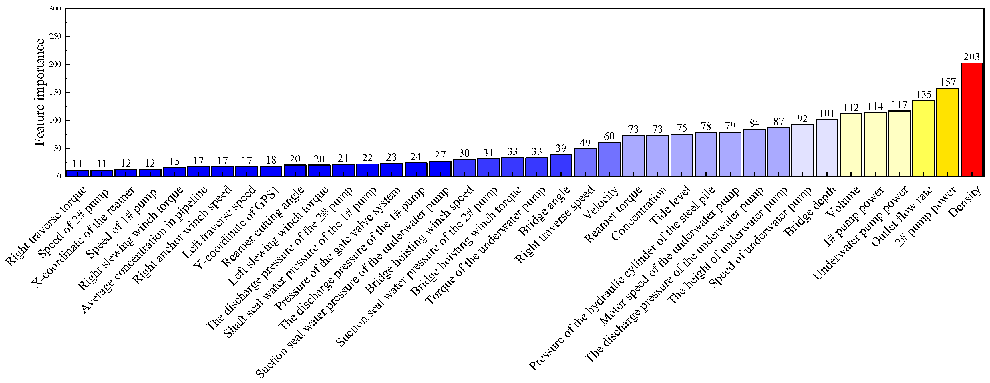
4. Correlation Analysis and Feature Selection

4.1. Data Normalization

In the process of carrying out the correlation analysis, the characteristic parameter terms between the different dimensions need to be compared. The original production data between different parameters are often on a different scale; the difference between the values may be very large, and not processing the data may affect the results of the data analysis. In this study, in order to avoid the influence of factors outside of the characteristic weight, the data need to be normalized before carrying out the correlation analysis of the preprocessed data for standardized processing [6]. Taking into account the fact that the numerical changes in the parameter items are not uniform, i.e., they have different distribution characteristics, we used the maximum and minimum normalization method to normalize the data, and the conversion formula is as follows [7]:

$$X^{*}=\frac{x-\min }{\max -x}$$

(2)

where max is the maximum value of the sample data, min is the minimum value of the sample data, and max − min is the extreme deviation.

The data used in this paper were statistically normalized to between 0 and 1, and some of the results are shown in Figure 9. The normalized data were distorted and were therefore only used for correlation analysis.

4.2. Correlation Analysis

The vacuum of underwater pumps is affected by several unknown factors, so it was decided to adopt a two-dimensional data visualization method, using the pairwise correlation matrix to present the correlation between each parameter in the form of a heat map. The color blocks of the heat map can be obtained by mapping the corresponding data values, and the strength of the correlation can be presented in an intuitive way by stipulating the mapping rule to vary with the size of the values. In this paper, Spearman’s correlation coefficient, which can reflect the correlation between the trend, direction, and the strength of random variables, was chosen for the data correlation analysis of this data mining process. Spearman’s correlation coefficient places no limitation on the sample capacity and overall distribution, so it has good applicability.

The object data set showed regional randomness locally, and certain monotonicity in general, and thus, it was decided to improve Spearman’s correlation coefficient method by combining it with information theory when analyzing the correlation of the data [8]. In the calculation based on Spearman’s correlation coefficient method, the order and level difference between the eigenvalues were mainly used. Spearman’s correlation formula is [9]:

$$\mathit{\rho }=\frac{{\displaystyle \sum _{\mathrm{i}=1}^n(x_i-}\overline{x})(y_i-\overline{y})}{\sqrt{{\displaystyle \sum _{\mathrm{i}=1}^n(x_i-}\overline{x}{)}^2+{\displaystyle \sum _{\mathrm{i}=1}^n(y_i-}\overline{y}{)}^2}}$$

(3)

where n is the sample size, $\mathit{\rho }$ is the correlation coefficient, and x and y are the corresponding elements in the two variables.

The subtraction of the corresponding elements of the two variables $x_i$ and $y_i$ observed here yields a difference, $d_i$. The above equation can then be transformed into:

$$\mathit{\rho }=1-\frac{6{\displaystyle \sum d_i^2}}{n({\mathrm{n}}^2-1)}$$

(4)

The correlation coefficient results are presented in the form of a heat map, and the results are shown in Figure 10. The values on the intersection position of the two parameter items represent their correlation coefficients. The larger the value, the redder the color, and the stronger the correlation is. On the contrary, the lower the value, the bluer the color of the square, which indicates that the correlation is weaker [10]. Because of the need to analyze several feature items, all feature items are numbered in the correlation analysis of this paper. No. 62 represents the underwater pump vacuum to be analyzed in this paper, and its correlation results with other feature items are expressed in the 62nd line with the intersection position of the other feature items.

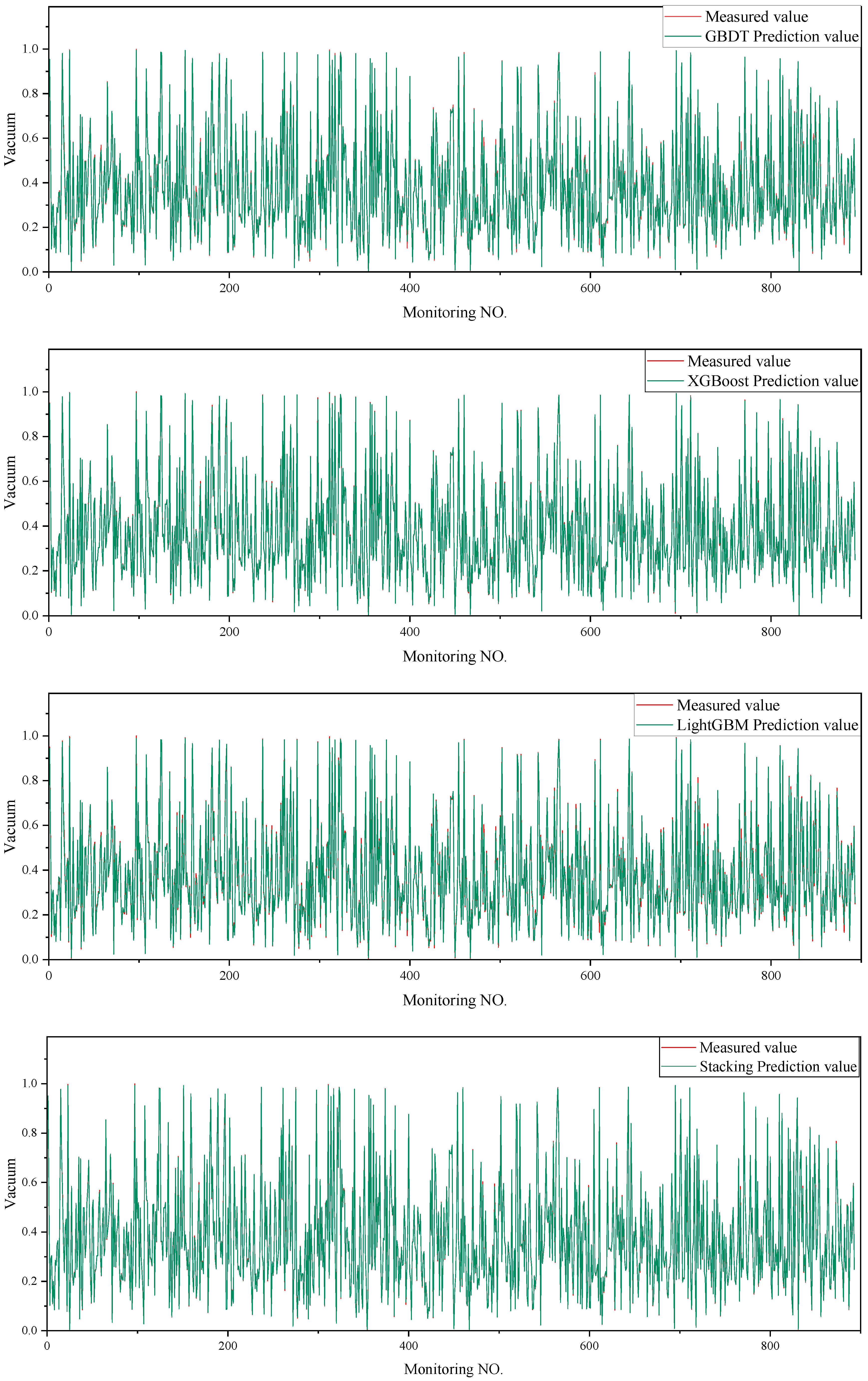
5. Model Training and Evaluation

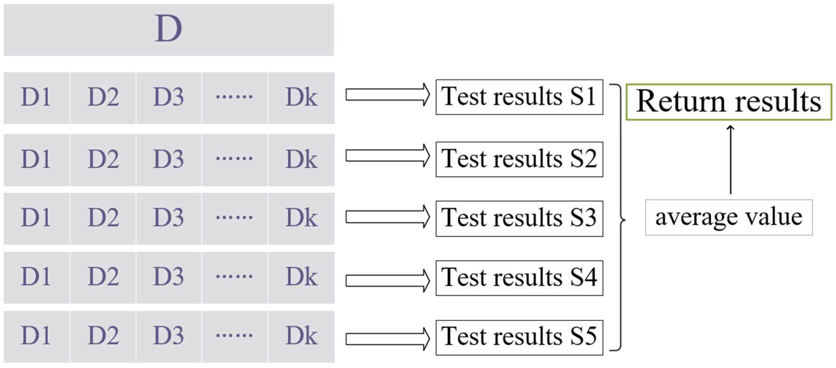
This research aimed to predict the vacuum degree of the underwater pump of a CSD based on the characteristics of the data collected from the CSD. We limited the use of supervised models and selected a variety of different models to compare their performance [11,12,13]. Considering that the feature volume data of this project present a random distribution within a finite interval, we decided to choose two linear regression models, three boosting decision tree models, and the stacking model for training and learning, as well as prediction evaluation, and we finally evaluated the applicability of each model with the help of various indicators. The purpose of using multiple single-mode integrated and stacking models for joint testing was to find a suitable technical solution for the vacuum prediction of a CSD. Considering that the dredging system is affected by many factors such as water pressure, piping system, and mud, the data distribution may have more randomness, so we decided to debug the multiple models jointly [14,15]. Considering the different distribution characteristics of each feature term in the data set, we finally determined the following models to be analyzed after combining the characteristics of each model.

5.1. Data Splitting

Before starting to train the model, the data need to be split into a training set and a test set, to avoid overfitting in the process of model training. In this study, the K-fold cross-validation method, the principle of which is shown in Figure 11, was chosen to split the data. The data set D was divided into K equal proportions, with one of the copies as the test data, and the other K-1 copies as the training data. Then, a different copy was used as the test set, and the other copies were subjected to relatively independent model training as the training set. The cross-validation was repeated K times until all individual copies had been used as the test data. Finally, the results of the K experiments were divided equally.

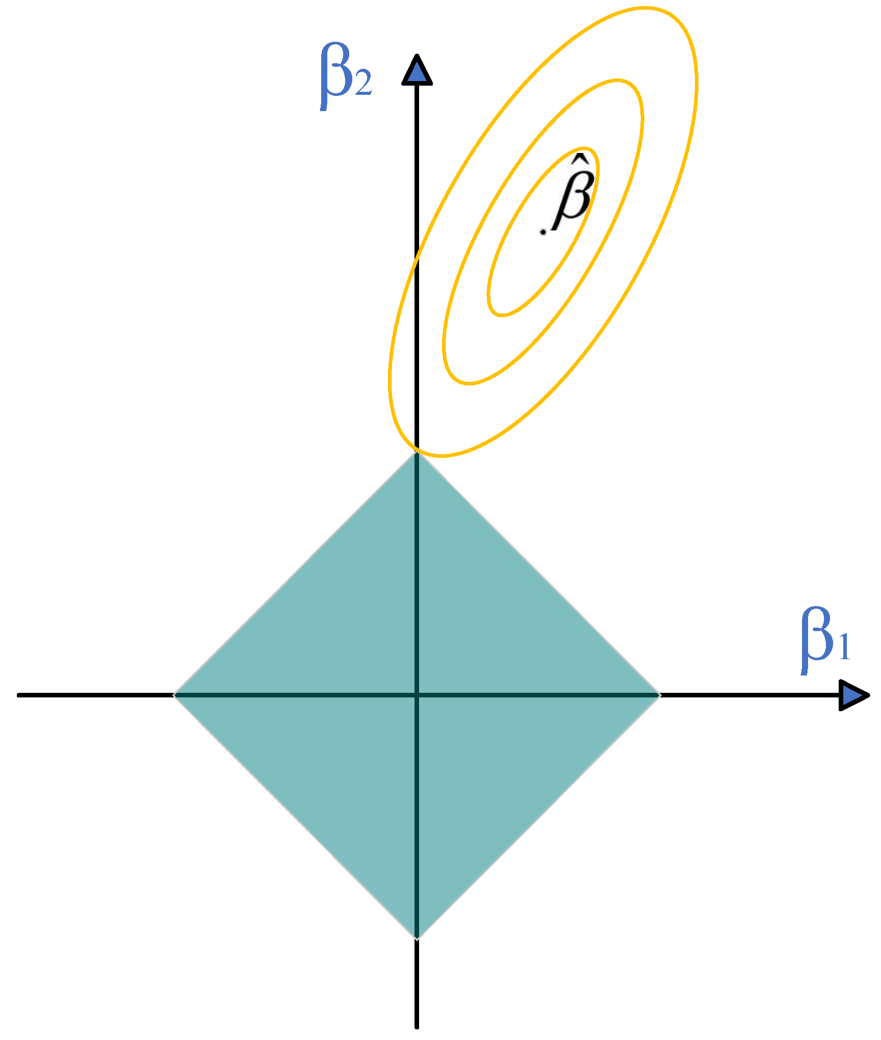
5.2. Lasso Regression

The lasso method is a compression estimation method that aims at reducing the set of variables. It controls the sparsity of the estimated coefficients through the alpha parameter. It reduces the regression coefficients to zero by penalizing the regression model with a penalty term of L1 regularization after the loss function, which is the sum of the absolute coefficients. For lasso estimation, the objective function is:

$${\widehat{\mathit{\beta }}}_{Lasso}=\underset{\mathit{\beta }\in R^d}{\arg \min }({‖Y-X\mathit{\beta }‖}^2+\mathit{\lambda }{\displaystyle \sum _{j=1}^d\left|{\mathit{\beta }}_j\right|})$$

(5)

Figure 12 shows the lasso regression estimation plot. The square area represents the constraint function area, and the yellow border line is the least squares error function contour. Because the constraint domain of lasso is square, this will produce points tangential to the coordinate axis, which causes some of the dimensional features to be weighted at 0. Therefore, it is easy to produce sparse results, so the lasso method can achieve the effect of variable selection, and the non-significant variable coefficients will be compressed to 0.

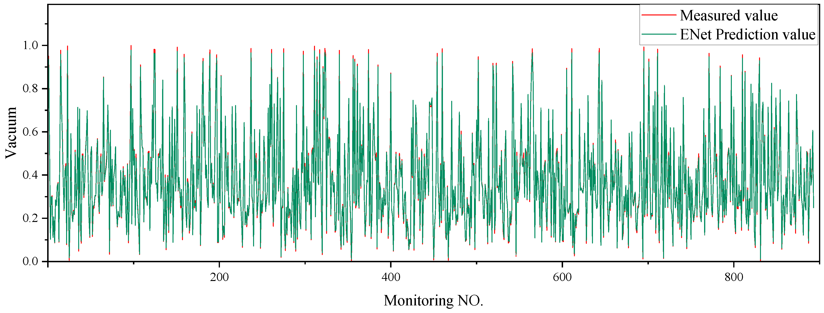
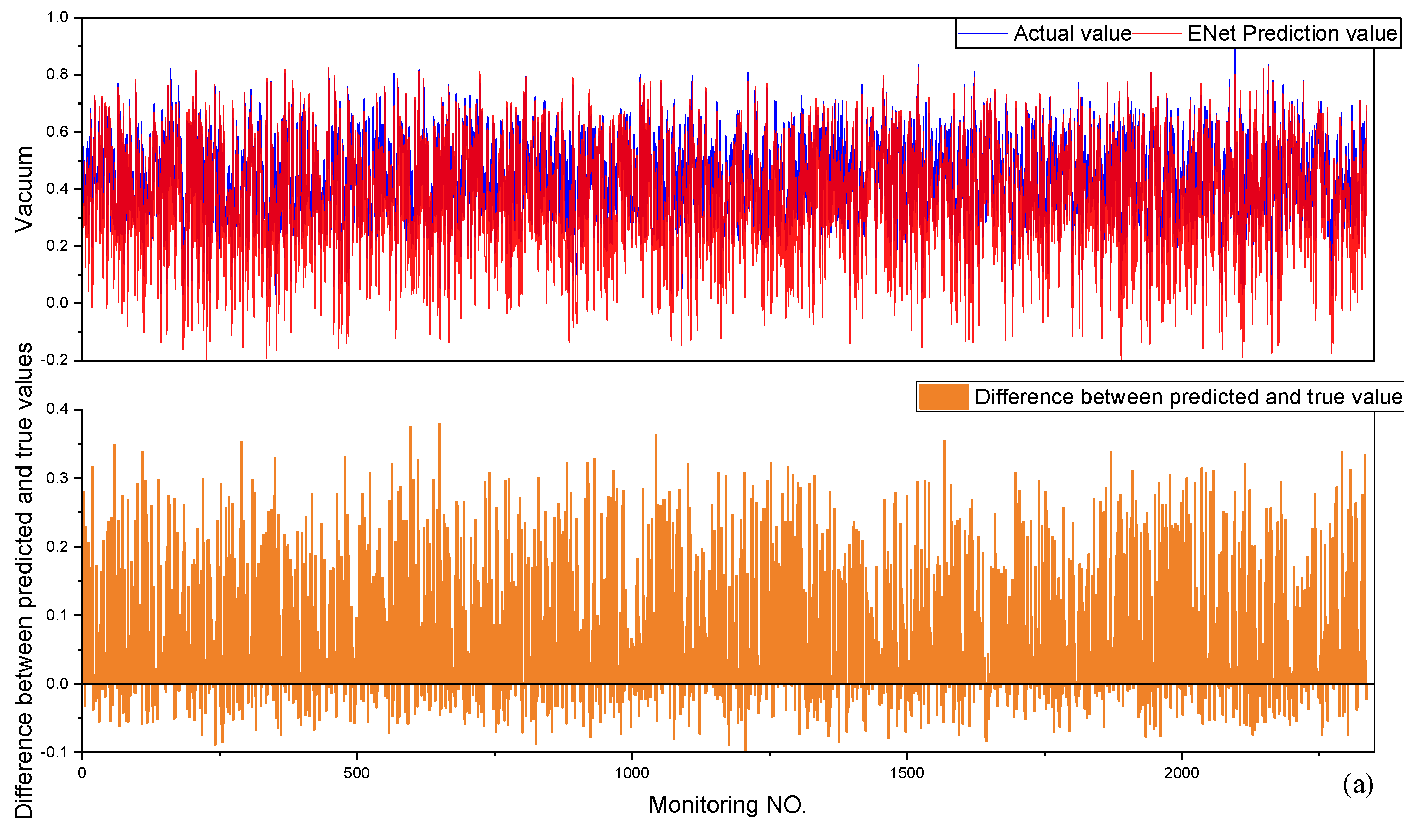
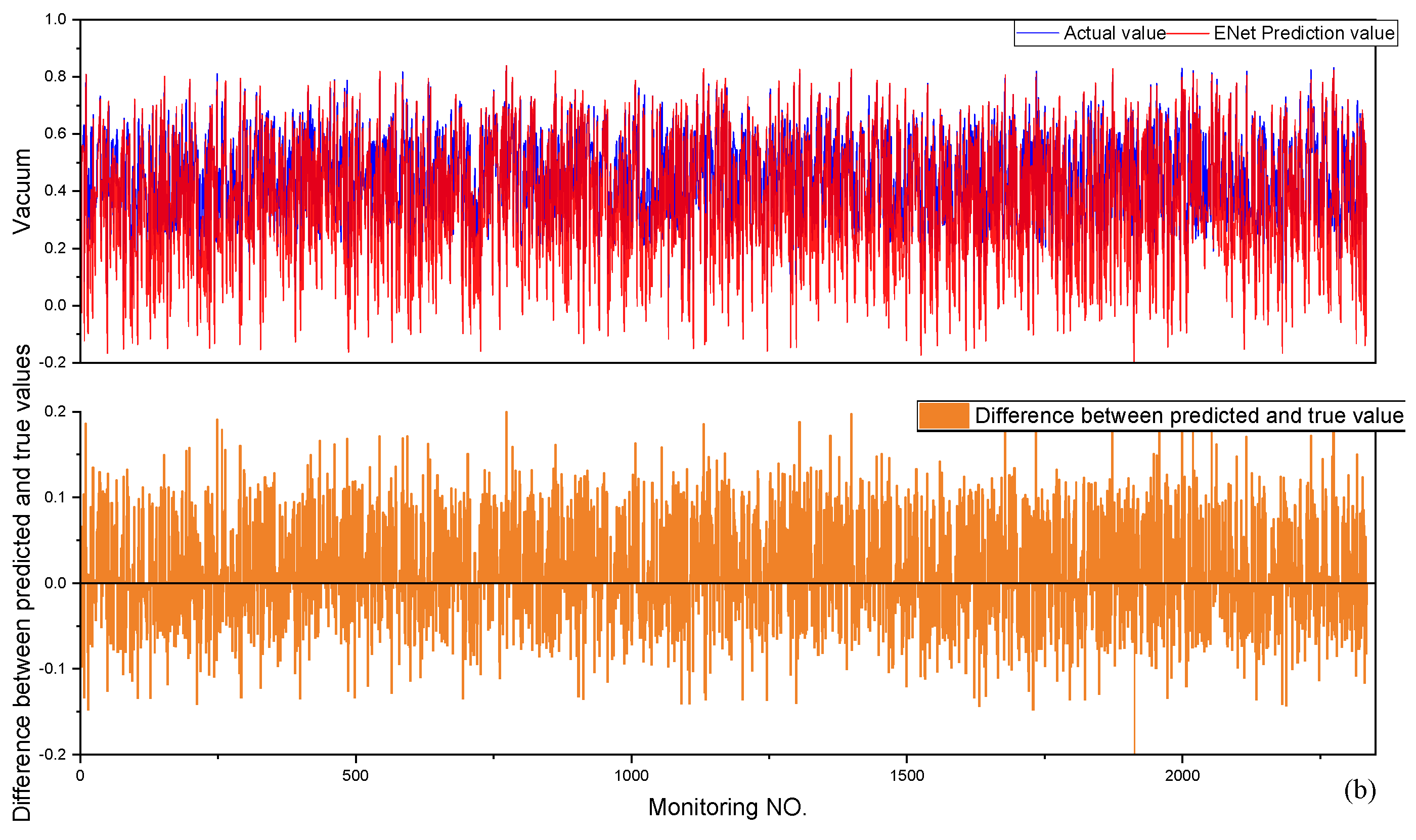
5.3. Elastic Network

The elastic network regression is a hybrid of lasso regression and ridge regression, which retains the characteristic of lasso that easily produces sparse solutions, but also combines some of the regular properties of ridge regression, and controls the size of the penalty term by two parameters χ and ρ [16]. The cost function is:

$$\mathrm{Cos}t(w)={{\displaystyle \sum _{i=1}^N(y_i-w^T{x}_i)}}^2+‘\mathit{\lambda }\mathit{\rho }{‖w‖}_1+\frac{\mathit{\lambda }(1-\mathit{\rho })}{2}{‖w‖}_2^2$$

(6)

When the cost function takes the minimum value,

$$w=\underset{w}{\arg \min }({\displaystyle \sum _{i=1}^N{(y_i-w^T{x}_i)}^2}+\mathit{\lambda }\mathit{\rho }{‖w‖}_1+\frac{\mathit{\lambda }(1-\mathit{\rho })}{2}{‖w‖}_2^2$$

(7)

ENet regression is suitable for data where there are multiple non-significant variables while still maintaining the regularization property. The ENet regression model works better when multiple variables are correlated with a particular variable. It removes invalid variables such as lasso regression while maintaining the stability of ridge regression. When ρ = 0, its cost function is equivalent to that of ridge regression, and when ρ = 1, its cost function is equivalent to that of lasso regression. As with lasso regression, the cost function has absolute values and is not always derivable, so there is no way to obtain the analytical solution of w by direct derivation, but we can still use the coordinate descent method to solve w.

5.4. Traditional GBDT

GBDT is a decision tree algorithm based on iterative accumulation, which constructs a set of weak learner trees and accumulates the results of multiple decision trees as the final prediction output, adopting the thinking of numerical optimization, and using the fastest descent method to solve the optimal solution of the loss function, which uses the CART decision tree to fit the negative gradient. Tree models are also divided into decision trees and regression trees; decision trees are often used to classify problems, and regression trees are often used to predict problems. GBDT is a linear combination of a set of weak learners, and it is initialized with a weak learner of:

$$f_0(x)=\arg \underset{c}{\min }={\displaystyle \sum _{i=1}^{N}L(y_i,c)}$$

(8)

For m = 1,2 …, M, the following steps apply.

(1)

For each sample (i = 1, 2 …, N), the residuals are calculated by:

$${\mathit{\gamma }}_{im}=-{\left[\frac{\mathit{\partial }L(y_i,f(x_i)}{\mathit{\partial }f(x_i)}\right]}_{f(x)=f_{m-1}()}$$

(9)

(2)

The residuals obtained in the previous step are used as the new true values of the samples, and the data $(x_i,x_{im})$ (i = 1, 2, …) are substituted to obtain a new regression tree, whose corresponding leaf node region is $R_{jm}$ (j = 1, 2, …), where J is the number of leaf nodes of the regression tree t.

(3)

The best fit for the leaf region is calculated as follows:

$${\mathit{\gamma }}_{jm}=\arg \underset{r}{\min }={\displaystyle \sum _{x_i\in R_{jm}}L(y_i,f_{m-1}(x_i))}+\mathit{\gamma }$$

(10)

(4)

The Strong Learner is updated as follows:

$$f_m(x)=f_{m-1}(x)+{\displaystyle \sum _{j=8}^J{\mathit{\gamma }}_{jm}I}$$

(11)

(5)

The Final Learner is calculated as follows:

$$f(x)=f_M(x)=f_0(x)+{\displaystyle \sum _{m=1}^M{\displaystyle \sum _{j=1}^J{\mathit{\gamma }}_{jm}I}}$$

(12)

Each weak prediction model generation of GBDT depends on the gradient direction of the loss function, and its main advantages are that (1) it can flexibly deal with various types of data, including continuous and discrete values; (2) it can use a number of loss functions which are very robust to outliers; and (3) it has a high accuracy rate with a relatively small number of tuning parameters.

5.5. Extreme Gradient Boosting

XGBoost is a model that uses stepwise forward additivity, which belongs to the boosting framework algorithm in integrated learning, with the advantage that there is no need to recalculate after generating weak learners in each iteration [17]. When a model does not perform well, one continues to train the second model according to the part of the original model that does not perform well, and so on. The underlying idea is the same as GBDT: through the construction of multiple base learners using an additive model, the deviation between the results of the previous base learners and the real value is learned; through the learning of multiple learners, the difference between the model value and the actual value is constantly reduced, and the final model prediction is the sum of the prediction results from all base learners [18].

The XGBoost algorithm optimizes the loss function structure by adding regular terms to the loss function, which can reduce the risk of overfitting to achieve the generation of weak learners. In addition, the XGBoost algorithm determines the structure of the tree and the score of all strong learners by directly using the first-order derivative and second-order derivative values of the loss function, and it greatly improves the performance of the algorithm through techniques such as pre-sorting, weighted quartiles, etc., which means that XGBoost is distinguished by the fact that it does not obtain the structure of the tree by fitting the residuals [19].

5.6. Light Gradient Boosting Machine

LightGBM is further optimized compared to XGBoost [20], mainly in the following aspects:

(1)

Introduction of the histogram algorithm. Continuous floating-point eigenvalues will be discretized into K integers, and at the same time, a histogram of width K will be constructed. When traversing the data, the discretized values will be used as indexes to accumulate statistics in the histogram. After traversing the data once, the histogram will be able to accumulate the required statistics, and then it will be traversed to find the optimal segmentation point according to the discrete values of the histogram [21].

(2)

Accelerated tree construction with the help of histogram difference. The histogram of a leaf can be obtained by the difference between the histogram of its father node and the histogram of its brother, which makes LightGBM twice as quick as other methods.

(3)

Leaf-wise leaf growth strategy with depth limitation. Most GBDT tools use the inefficient level-wise decision tree growth strategy to treat leaves in the same layer indiscriminately, which brings a lot of unnecessary overhead. In fact, many leaves have low splitting gain, and there is no need to search and split them, while LightGBM uses a depth-constrained grow-by-leaf algorithm.

(4)

One-sided gradient sampling algorithm. LightGBM is an algorithm that can better balance the amount of data and accuracy, from the point of view of reducing samples, excluding most of the small gradient samples, and using only the remaining samples to calculate the information gain.

(5)

Mutually exclusive feature bundling algorithm. LightGBM reduces the feature dimensions by means of feature bundling to improve computational efficiency. Usually, the bundled features are mutually exclusive, so that two bundled features will not lose information [22].

5.7. Stacking Model

The purpose of integrated learning is to obtain a strong model by combining many weak models, as shown in Figure 13, where y1, y2, and y3 represent three base models, and x and y represent the target term and the set of feature parameters. The model first learns the original data through the base learners, and models the stack of the original fitted data. Then, all these base learners output the original data, and the outputs of these models are stacked in columns to form (m, p)-dimensional new data, with m representing the number of samples and p representing the number of base learners. Finally, the new sample data are given to the second layer model for fitting [23,24,25].

Here is an example of the training process for stacked models. For the first model (model 1) to be integrated, if we use k fold cross-validation, we will have to train k times for the same type of model 1. Under the cross-validation split, the training set and test set are different each time, so the output produced by each training iteration is also different. Therefore, after we complete the training based on model 1, we will obtain an output of the same size as the feature items, and we will add them together to obtain the mean of the prediction results of model 1 on the original data. Repeating this for each base model gives us the second layer of the data set.

6. Analysis of Results of Model Training

6.1. Model Parameter Optimization

To propose a new vacuum prediction method for underwater pumps, 56 feature terms were selected as input variables affecting the vacuum level to participate in the training and testing of the six models described above. These parameters were partitioned into five crosses for training algorithms and model testing by the cross-validation method [26]. The main parameter choices in the six models will be explained in this section.

Table 2. Parameters of several selected models.

Model	Parameters
Lasso	α = 0.1; max_iter = 50
Enet	α = 0.01; L1_ratio = 0.003; random_state = 3
GBDT	rate = 0.05; max_depth = 4; n_estimators = 3000
XGBoost	rate = 0.05; max_depth = 3; n_estimators = 2200
LightGBM	rate = 0.05; n_estimators = 720; max_bin = 55; num_leaves = 5

shows a summary of the main parameters of each model [27].

Analyzing these parameters is beneficial for understanding the characteristics of each model, and thus choosing a more appropriate scheme. The settings of lasso regression include parameters such as the L1 regular term coefficient, the maximum number of iterations, and whether or not to normalize the data by the L2 paradigm. The elastic network includes the penalty term coefficient, regular term coefficient and alpha value, etc., in which the L1_ratio determines the penalty term of the elastic network. LGBM and GBDT contain important parameters such as the maximum tree depth, the minimum number of samples, the maximum number of nodes, the learning rate, and the L1 and L2 regular term coefficients in XGBoost and LGBM. The fitting effect and convergence speed during model training can be controlled by adjusting the above parameters, which can help us find a suitable prediction model.

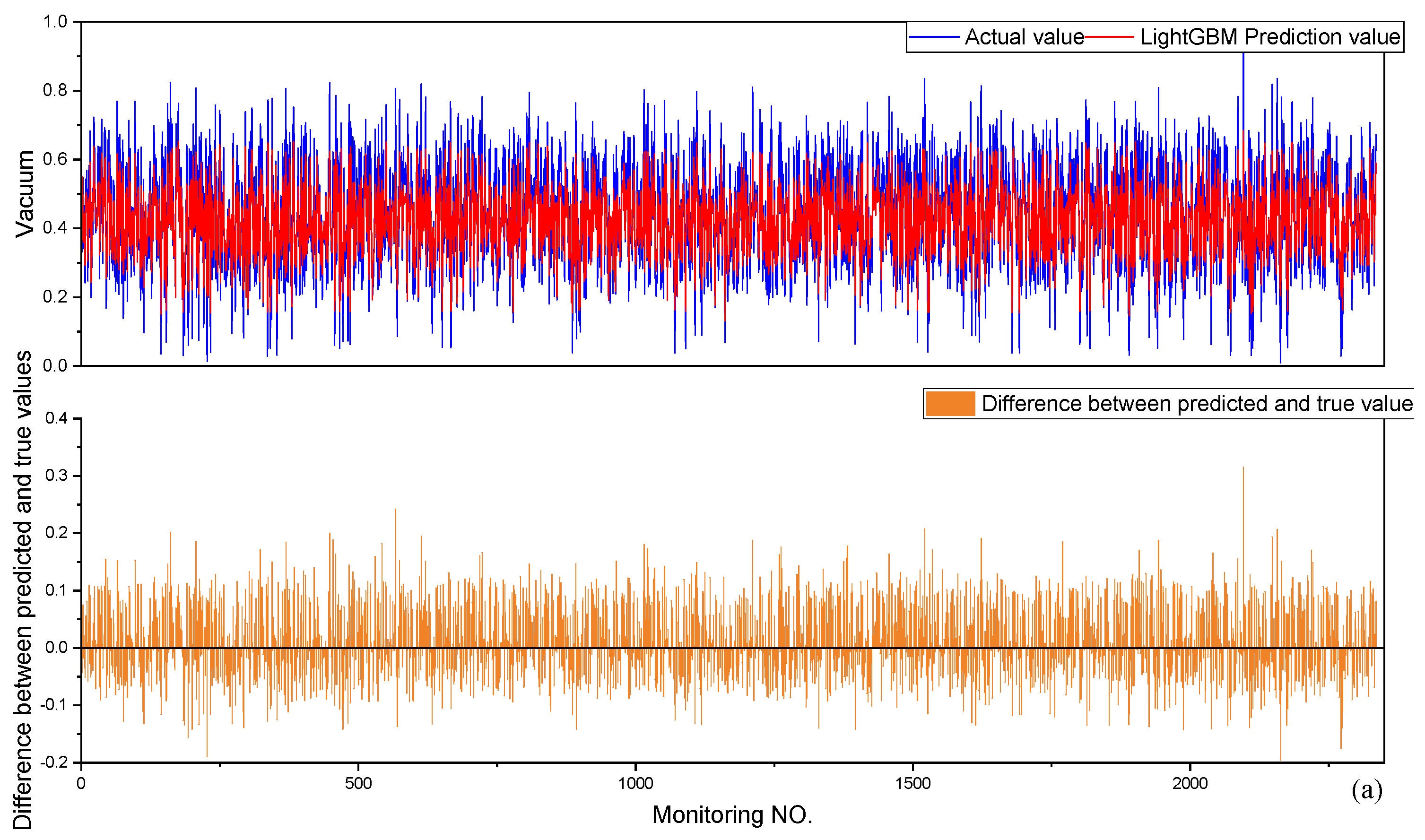
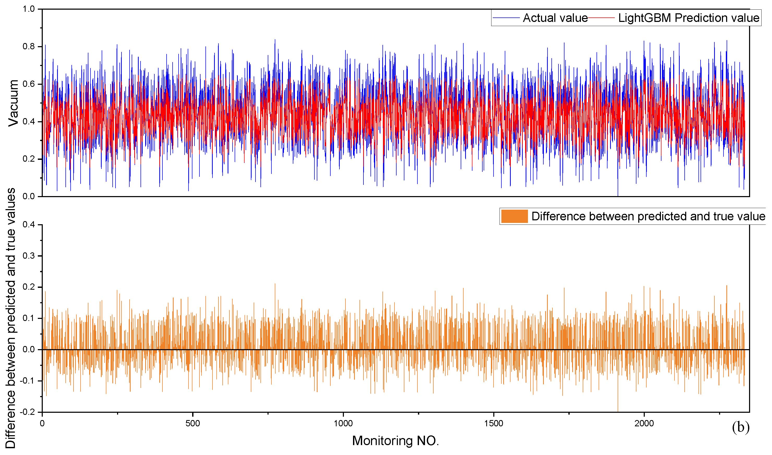
6.2. Model Evaluation

In this paper, the route of selecting the final prediction model is based on the comparative evaluation of multiple models. Therefore, in order to show the performance of each model intuitively, so as to have a more objective basis of judgment in the comparative analysis, this paper uses the three indexes of Root Mean Squared Error (RMSE), Mean Absolute Error (MAE), and degree of fitting ($R^2$) for the comprehensive evaluation of each model algorithm. RMSE mainly measures the deviation between the predicted value and the real value: the smaller the RMSE value is, the higher the prediction accuracy is. MAE represents the average of the absolute error between the predicted value and the real value, which can reflect the real situation of the prediction error, and the bigger the prediction error is, the bigger the value is. The above two evaluation indexes can only be used for the results of the same outline, and it is difficult to make an evaluation when the outline is different. However, $R^2$ can effectively reflect the differences between different models, and the closer $R^2$ is to 1, the better the fit of the model to the data is [28]. In the examination of vacuum prediction methods, obtaining accurate model prediction results is the foundation of the research work, while the fitting speed of the model will affect the speed of real-time data updating in engineering. In this study, the running time of the code in the evaluation process was also an indicator of concern.

The performance of the trained model in relation to the test data is shown in

Table 3. Performances of different algorithms.

Modal	${\mathit{R}}^2$	MAE	RMSE	Time
Lasso	−0.000791	0.128561	0.160684	0.00099
ENET	0.997402	0.006231	0.008186	0.0360
GBDT	0.995463	0.008021	0.010819	12.7307
XGBoost	0.987243	0.012969	0.018142	0.4404
LightGBM	0.995764	0.008163	0.010454	0.1225
Stacking	0.997833	0.128561	0.007478	11.8235

. It can be noted that the lasso model still has a negative $R^2$ value of 0.1. At this time, the model fits the data very poorly, the error of the fitting function is larger than that of the mean function, and the fitting results have lost their practical reference significance. The value of the χ range is 0~1. In this study, we tested the fit of χ less than 0.1 and predicted that the fit of the model would gradually improve as the value of χ decreased, but it only showed better accuracy close to 0, which shows that the lasso regression model using the regularized penalty term is not applicable to the data mining of this data set.

GBDT and stacking achieve a better fit, but both of them take more than 10 s, much longer than the other models. The ENET model and LightGBM model show a better timeliness and fitting effect in the prediction process; both of them lose part of the accuracy, but greatly accelerate the speed of convergence of the model. In particular, ENET achieves faster convergence with better fitting data and higher accuracy. Therefore, it is recommended to use the ENET model and LightGBM model to carry out underwater pump vacuum prediction, which can help to reduce the hardware requirements, obtain a high frequency of acquisition and prediction, and reduce the data delay; engineering applicability is also better [29,30].

In this paper, to visualize the difference in the prediction accuracy of each algorithmic model, we have drawn a curve diagram comparing the test set of the corresponding algorithmic model with the prediction data, as shown in Figure 14, where the red line represents the test data, and the green line corresponds to the prediction data of the corresponding model. It can be seen from this diagram that the difference in the prediction accuracy of the models is not large. The best performance of the stacking model and the second-best performance of the ENET model are due to the fact that both models have a better fitting performance in the mutation points with large deviations, or in the regions with a more concentrated distribution of the data. However, the overfitting phenomenon in the mutation points of the stacking model and the ENET model cannot be excluded in light of the abnormal mutations in the original data. In terms of performance, GBDT and LightGBM are close to each other, and both of them achieve poorer fitting performance in the mutation points. Finally, XGBoost has the worst performance, and its prediction value is different from that of the test set, showing discrepancies at multiple points.

In order to study the importance of each data item for the prediction of underwater pump vacuum, this project used the LightGBM algorithm to calculate the importance of 56 parameters other than the vacuum in the model prediction process. Of these, 38 features show obvious influence in the process of model training, as shown in Figure 15, where the values are dimensionless quantities, and the difference in the size of the relative influence corresponds to the magnitude of the performance. From this, it can be seen that in the prediction of underwater pump vacuum, density and 2# pump power are very important. In addition, the outlet flow rate, compass angle, underwater pump power, and 1# mud pump power are also important, while the importance of the volume, bridge depth, and underwater pump speed cannot be ignored. The above seven features show a strong influence in the process of underwater pump vacuum prediction, while from the previous correlation analysis, we know that there is a strong correlation between vacuum and volume, density, underwater pump speed, bridge depth, outlet flow rate, concentration, flow rate, underwater pump power, 1# pump power, and 2# pump power. It has been stated that the size of the correlation coefficient in the actual prediction stage is the basic criterion for the initial feature screening, and here, the results of the correlation analysis are combined with the prediction results to show that density, volume, outlet flow rate, concentration, flow rate, underwater pump power, 1# pump power, and 2# pump power have a greater impact on the prediction effect of the underwater pump vacuum degree.

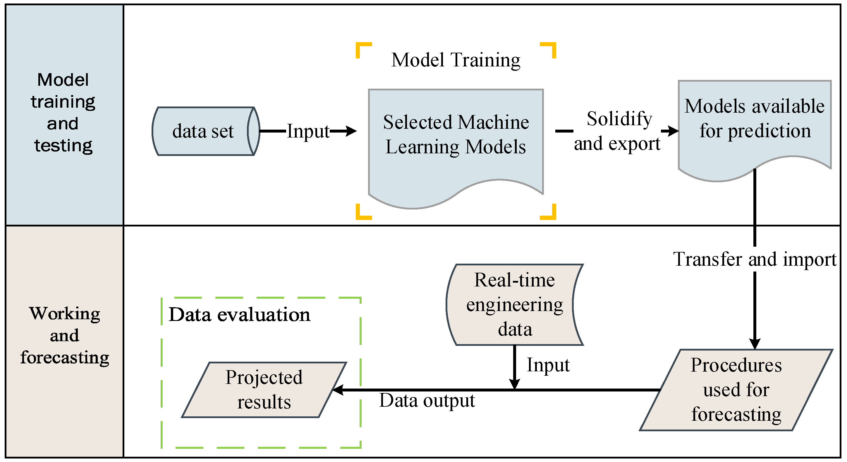
7. Model Generalization Capability Assessment and Application Methods

In the process of vacuum prediction using trained models, the models that have been learned in the training data will be based on real data to carry out the prediction, which requires knowing whether the models that have completed the training are able to perform adequately using the brand-new data. In this section, we will derive and assess the generalization ability of the proposed model based on two well-performing training models.

7.1. Assessment of Generalization Capacity

In the previous section on model training evaluation, it was mentioned that stacking and ENET had a better fit, but there might be overfitting, and the GBDT and the LightGBM had better accuracy. Considering that the convergence speed of GBDT and the stacking model is too slow, it was decided to use ENET and LightGBM as the models for generalization ability evaluation. We chose to export ENET and LightGBM in the PKL file format, and further carried out generalization tests on them [31].

The generalization test is based on another data set, where the data will be used to predict the vacuum level based on the rules of the models obtained from machine learning, and the results will be compared with the theoretically calculated values. For this generalization test, two splits of the data were chosen to assess the stability of the model, which also facilitates the determination of the influence of random variables. Figure 16 and Figure 17 plot the theoretical values against the predicted data of the ENET and LightGBM models, respectively, where the blue line represents the real data and the red line represents the predicted data for the corresponding model.

What can be seen from the prediction comparison graph is that LightGBM shows a better fit between the predicted values and the true values, which proves that it has a better generalization ability. On the other hand, ENET shows a large deviation, which corresponds to a large discrepancy with the results of the model training process. This proves that the ENET model has been overfitted during the model training process and thus has a poor generalization ability. We also assessed the statistics for the corresponding evaluation indexes, and the results are shown in

Table 4. Performance of the chosen model in generalization tests.

Model	${\mathit{R}}^2$	MAE	RMSE	MSE
ENET	0.45282	0.09224	0.12548	0.01574
	0.46916	0.09191	0.12522	0.01568
LightGBM	0.82507	0.05839	0.07095	0.005034
	0.82427	0.05991	0.07204	0.005190

.

Based on the evaluation metrics, it can be seen that LightGBM shows better accuracy compared to ENET, and its better fitting indicates a better generalization ability.

7.2. Engineering Methods

Considering the complexity of the actual engineering environment, as well as the pressure of model training on the equipment environment, in this study, we decided to evaluate the training and prediction of a variety of machine models. At the same time, the model training and vacuum prediction were designed as relatively independent work modules, and the predictive model was stored in a file between model training and validation use. By separating the model training and learning from the engineering use, the method has the flexibility required for the engineering application, but it also places higher requirements on the imported data. As shown in Figure 18, the method proposed in this paper takes model training as the work content of the shore operation, the offshore module is the module with the prediction function, and the model is overwritten by importing the model file, which can be realized through a variety of file transfer methods. The technical approach provided in this paper requires that the feature items imported by the shipboard prediction program be consistent with the feature items of the data set used for model training, which includes the format, number, and content of the feature item indexes, since differences in the feature items may lead to compatibility problems with the model.

8. Conclusions

For the CSD, the vacuum degree of the underwater pump is often closely related to the operational efficiency. The operational efficiency can be improved by controlling the vacuum degree within a range, and the vacuum degree has good reference value for providing early warnings of pipeline blockages. This study used existing engineering construction data to train a variety of machine learning models and correspondingly evaluate their performance, and multiple rounds of data were used to train and test the machine learning models selected in this paper. To verify the technical stability of the method proposed in this paper, we provide a technical solution that can help to realize the prediction of the vacuum of an underwater pump.

It should be explained that this study was carried out using engineering data for a limited capacity. The data set used may not fully reflect the various operating conditions that CSDs will encounter in the project, which may affect the models derived from them. The impact still needs to be studied. The research presented in this paper explored real vacuum prediction under limited calibration feature parameter items, and this work depended on the use of a large number of data sets to repeat training; therefore, the method proposed in this paper is not clearly defined in terms of the characteristic items and data volume. If there are insufficient data, the effects demonstrated in this study cannot be achieved.

The main work and conclusions of this study are as follows:

(1)

In this paper, theoretical engineering experience and Spearman’s correlation coefficient were jointly introduced into the feature selection process to reduce the dimensionality of the data;

(2)

This research included several rounds of training and testing similar to the work mentioned in this paper using several different datasets, and in the evaluation phase, we found that the results were similar to the experimental results presented in this paper, which supports the use of the model selection scheme we propose;

(3)

The results of the analysis in this study show that the main factors influencing the change in the vacuum level of the underwater pump of the CSD are the density, the flow rate, the bridge depth, the 1# pump power, the 2# pump power, the underwater pump power, the speed of the underwater pump and the height of the underwater pump;

(4)

In this paper, we propose evaluating the generalization ability based on the preferred model. We compared the generalization ability of the models with better performance in model training, and verified that LightGBM is suitable for predicting the vacuum level of the underwater pump of a CSD, as well as verifying the engineering feasibility of the method;

(5)

This paper proposes an engineering method for predicting the vacuum level of the underwater pump of a suction dredger based on the analyzed data, and also accordingly proposes a feasible engineering application scheme.

References

1. Wang, B.; Fan, S.D.; Jiang, P.; Xing, T.; Fang, Z.L.; Wen, Q. Research on predicting the productivity of cutter suction dredgers based on data mining with model stacked generalization. Ocean Eng. 2020, 217, 108001. [Google Scholar] [CrossRef]
2. Bai, S.; Li, M.C.; Kong, R.; Han, S.; Li, H.; Qin, L. Data mining approach to construction productivity prediction for cutter suction dredgers. Autom. Constr. 2019, 105, 102833. [Google Scholar] [CrossRef]
3. Li, M.C.; Lu, Q.R.; Bai, S.; Zhang, M.X.; Tian, H.J.; Qin, L. Digital twin-driven virtual sensor approach for safe construction operations of trailing suction hopper dredger. Autom. Constr. 2021, 132, 103961. [Google Scholar] [CrossRef]
4. Han, S.; Li, H.; Li, M.C.; Tian, H.J.; Qin, L.; Yu, Y.; Ma, J. Intelligent short-term forecasting for mud concentration in CSD dredging construction. Ocean Eng. 2022, 266, 113151. [Google Scholar] [CrossRef]
5. Booyse, W.; Wilke, D.N.; Heyns, S. Deep digital twins for detection, diagnostics and prognostics. Mech. Syst. Signal Process. 2020, 140, 106612. [Google Scholar] [CrossRef]
6. Shang, G.; Xu, L.Y.; Tian, J.Z.; Cai, D.W.; Xu, Z.; Zhou, Z. A real-time green construction optimization strategy for engineering vessels considering fuel consumption and productivity: A case study on a cutter suction dredger. Energy 2023, 274, 127326. [Google Scholar] [CrossRef]
7. Lima, F.T.; Souza, V.M.A. A Large Comparison of Normalization Methods on Time Series. Big Data Res. 2023, 34, 100407. [Google Scholar] [CrossRef]
8. Schober, P.; Boer, C.; Schwarte, L.A. Correlation Coefficients: Appropriate Use and Interpretation. Anesth. Analg. 2018, 126, 1763–1768. [Google Scholar] [CrossRef] [PubMed]
9. Szmidt, E.; Kacprzyk, J.; Galichet, S.; Montero, J.; Mauris, G. The Spearman and Kendall rank correlation coefficients between intuitionistic fuzzy sets. In Proceedings of the 7th Conference of the European Society for Fuzzy Logic and Technology (EUSFLAT-2011) and LFA-2011, Aix-Les-Bains, France, 18–22 July 2011; pp. 521–528. [Google Scholar]
10. Kou, G.; Lu, Y.Q.; Peng, Y.; Shi, Y. Evaluation of Classification Algorithms Using Mcdm and Rank Correlation. Int. J. Inf. Technol. Decis. Mak. 2012, 11, 197–225. [Google Scholar] [CrossRef]
11. Xu, W.; Kang, Y.; Chen, L.; Wang, L.; Qin, C.; Zhang, L.; Liang, D.; Wu, C.; Zhang, W. Dynamic assessment of slope stability based on multi-source monitoring data and ensemble learning approaches: A case study of Jiuxianping landslide. Geol. J. 2023, 58, 2353–2371. [Google Scholar] [CrossRef]
12. Liang, X.Y.; Jacobucci, R. Regularized Structural Equation Modeling to Detect Measurement Bias: Evaluation of Lasso, Adaptive Lasso, and Elastic Net. Struct. Equ. Model. A Multidiscip. J. 2020, 27, 722–734. [Google Scholar] [CrossRef]
13. Liang, W.Z.; Luo, S.Z.; Zhao, G.Y.; Wu, H. Predicting Hard Rock Pillar Stability Using GBDT, XGBoost, and LightGBM Algorithms. Mathematics 2020, 8, 765. [Google Scholar] [CrossRef]
14. Luo, X.; Xu, L.; Huang, P.; Wang, Y.; Liu, J.; Hu, Y.; Wang, P.; Kang, Z. Nondestructive Testing Model of Tea Polyphenols Based on Hyperspectral Technology Combined with Chemometric Methods. Agriculture 2021, 11, 673. [Google Scholar] [CrossRef]
15. Wang, X.; Yang, Y.; Liu, J.; Wang, G. The stacking strategy-based hybrid framework for identifying non-coding RNAs. Brief. Bioinform. 2021, 22, bbab023. [Google Scholar] [CrossRef] [PubMed]
16. Khan, A.Z. Regularization and Variable Selection via the Fixed-Shape Elastic Net and Exponential Norm. Master’s Thesis, King Fahd University of Petroleum and Minerals, Dhahran, Saudi Arabia, 2017. [Google Scholar]
17. Zhang, W.; Wu, C.; Zhong, H.; Li, Y.; Wang, L. Prediction of undrained shear strength using extreme gradient boosting and random forest based on Bayesian optimization. Geosci. Front. 2021, 12, 469–477. [Google Scholar] [CrossRef]
18. Chen, T.Q.; Guestrin, C.; Assoc Comp, M. XGBoost: A Scalable Tree Boosting System. In Proceedings of the KDD’16: The 22nd ACM SIGKDD International Conference on Knowledge Discovery and Data Mining, San Francisco, CA, USA, 13–17 August 2016; pp. 785–794. [Google Scholar]
19. Zhou, J.; Qiu, Y.; Zhu, S.; Armaghani, D.J.; Khandelwal, M.; Mohamad, E.T. Estimation of the TBM advance rate under hard rock conditions using XGBoost and Bayesian optimization. Undergr. Space 2021, 6, 506–515. [Google Scholar] [CrossRef]
20. Ke, G.L.; Meng, Q.; Finley, T.; Wang, T.F.; Chen, W.; Ma, W.D.; Ye, Q.W.; Liu, T.Y. LightGBM: A Highly Efficient Gradient Boosting Decision Tree. In Proceedings of the Advances in Neural Information Processing Systems 30 (NIPS 2017), Long Beach, CA, USA, 4–9 December 2017. [Google Scholar]
21. Friedman, J.H. Greedy function approximation: A gradient boosting machine. Ann. Stat. 2001, 29, 1189–1232. [Google Scholar] [CrossRef]
22. Hajihosseinlou, M.; Maghsoudi, A.; Ghezelbash, R. A Novel Scheme for Mapping of MVT-Type Pb-Zn Prospectivity: LightGBM, a Highly Efficient Gradient Boosting Decision Tree Machine Learning Algorithm. Nat. Resour. Res. 2023, 32, 2417–2438. [Google Scholar] [CrossRef]
23. Goh, K.L.; Goto, A.; Lu, Y. LGB-Stack: Stacked Generalization with LightGBM for Highly Accurate Predictions of Polymer Bandgap. ACS Omega 2022, 7, 29787–29793. [Google Scholar] [CrossRef]
24. Naimi, A.I.; Balzer, L.B. Stacked generalization: An introduction to super learning. Eur. J. Epidemiol. 2018, 33, 459–464. [Google Scholar] [CrossRef]
25. Paz Sesmero, M.; Ledezma, A.I.; Sanchis, A. Generating ensembles of heterogeneous classifiers using Stacked Generalization. Wiley Interdiscip. Rev. Data Min. Knowl. Discov. 2015, 5, 21–34. [Google Scholar] [CrossRef]
26. Bai, S.; Li, M.; Song, L.; Ren, Q.; Qin, L.; Fu, J. Productivity analysis of trailing suction hopper dredgers using stacking strategy. Autom. Constr. 2021, 122, 103470. [Google Scholar] [CrossRef]
27. Wang, B.; Fan, S.D.; Jiang, P.; Chen, Y.; Zhu, H.H.; Xiong, T. Cutting state estimation and time series prediction using deep learning for Cutter Suction Dredger. Appl. Ocean Res. 2023, 134, 103515. [Google Scholar] [CrossRef]
28. Huang, H.; Li, J.; Yang, H.; Wang, B.; Gao, R.; Luo, M.; Li, W.; Zhang, G.; Liu, L. Research on prediction methods of formation pore pressure based on machine learning. Energy Sci. Eng. 2022, 10, 1886–1901. [Google Scholar] [CrossRef]
29. Takele, Z.B.Z. Metaheuristic Based Stacked Generalization Algorithm. Master’s Thesis, State University of New York at Binghamton, Binghamton, NY, USA, 2018. [Google Scholar]
30. Zhang, Y.; Wen, M.; Sun, Y.; Chen, H.; Cai, Y. Black Carbon Emission Prediction of Diesel Engine Using Stacked Generalization. Atmosphere 2022, 13, 1855. [Google Scholar] [CrossRef]
31. Sandim, M.O. Using Stacked Generalization for Anomaly Detection. Master’s Thesis, Faculdade de Engenharia da Universidade do Porto, Porto, Portugal, 2017. [Google Scholar]
Figure 1. “Hua An Long”. Data acquisition and testing platform and its pipeline system.
Processes 12 00812 g001
Figure 2. Schematic diagram of the calculation term for underwater pump vacuum parameters.
Processes 12 00812 g002
Figure 3. Process of researching vacuum predicting methods for CSD underwater pumps.
Processes 12 00812 g003
Figure 4. Monitoring of changes in shaft seal water pressure.
Processes 12 00812 g004
Figure 5. Monitoring of changes in suction seal water pressure.
Processes 12 00812 g005
Figure 6. Monitoring of pump power changes.
Processes 12 00812 g006
Figure 7. Raw data box diagram.
Processes 12 00812 g007
Figure 8. Boxplot of cleaned data.
Processes 12 00812 g008
Figure 9. Partially normalized data.
Processes 12 00812 g009
Figure 10. Feature correlation heat map.
Processes 12 00812 g010
Figure 11. Principles of the cross-validation method of analyzing processes.
Processes 12 00812 g011
Figure 12. Lasso regression estimation plot.
Processes 12 00812 g012
Figure 13. Stacking principle schematic.
Processes 12 00812 g013
Figure 14. The fitting results of several models.
Processes 12 00812 g014aProcesses 12 00812 g014b
Figure 15. Feature importance.
Processes 12 00812 g015
Figure 16. Two rounds of generalization test results for ENet. (a) Prediction result of Enet based on one dataset. (b) Predictions of Enet based on the other dataset.
Processes 12 00812 g016aProcesses 12 00812 g016b
Figure 17. Two rounds of generalization test results for LightGBM. (a) Prediction result of LightGBM based on one dataset. (b) Predictions of LightGBM based on the other dataset.
Processes 12 00812 g017aProcesses 12 00812 g017b
Figure 18. Components of the engineering approach.
Processes 12 00812 g018