A Fault Diagnosis Method for Ultrasonic Flow Meters Based on KPCA-CLSSA-SVM

Abstract

To enhance the fault diagnosis capability for ultrasonic liquid flow meters and refine the fault diagnosis accuracy of support vector machines, we employ Levy flight to augment the global search proficiency. By utilizing circle chaotic mapping to establish the starting locations of sparrows and refining the sparrow position with the highest fitness value, we propose an enhanced sparrow search algorithm termed CLSSA. Subsequently, we optimize the parameters of support vector machines using this algorithm. A support vector machine classifier based on CLSSA has been constructed. Given the intricate data collected from ultrasonic liquid flow meters for diagnostic purposes, the approach of employing KPCA to decrease data dimensionality is implemented, and a KPCA-CLSSA-SVM algorithm is proposed to achieve fault diagnosis in ultrasonic flow meters. By using UCI datasets, the findings indicate that KPCA-CLSSA-SVM achieves fault diagnosis accuracies of 94.12%, 100.00%, 97.30%, and 100% in the four flow meters, respectively. Compared with the Bayesian classifier diagnostic algorithm, this has been increased by 4.18%. And compared with support vector machine diagnostic algorithms improved by the SSA, it has increased by 2.28%.

1. Introduction

In the petroleum industry, the basis for trade settlement between trading parties is the flow of oil, which puts forward high requirements for the measurement technology for oil. Ultrasonic flow meters have gradually replaced traditional flow meters due to their advantages of high accuracy, high sensitivity, no pressure loss, and good repeatability. They are the preferred instrument for measuring the flow rate of liquids with strong corrosion, poor conductivity, and high viscosity. Whether in industrial production, transportation, or long-term use, ultrasonic flow meters may experience various malfunctions, such as sensor failures, gas injection, waxing, etc. In addition, the installation effect of ultrasonic flow meters can also have a certain impact on the measurement of flow. These faults can lead to a decrease in the performance of ultrasonic flow meters, resulting in incorrect readings and the inability to provide guarantees for fair trade. Therefore, designing a fault diagnosis method to timely and accurately diagnose the types of faults present in ultrasonic flow meters is of great significance for the practical use of ultrasonic flow meters.

The traditional diagnostic methods for equipment faults generally start from the principles of the equipment itself and then combine these principles with the experience of experts to achieve the judgment and maintenance of equipment faults. The method of diagnosing abnormal equipment states based on the temperature changes of components is widely used in the fault diagnosis of wind turbines [1]. Vibration signals, lubricating oil analysis, and acoustic emission are used to detect faults in rolling bearings, large pumping station units, and motors [2,3,4,5]. However, with the rise of equipment manufacturing processes and the increase in their complexity, such methods based on the principles of the equipment itself not only need to comprehensively consider the influence of multiple relevant factors, but they also put forward high requirements for experts and their experience and analytical ability in fault diagnosis. Therefore, the efficiency and accuracy of fault diagnosis cannot be guaranteed.

In recent years, some scholars have used Bayesian methods to diagnose whether an equipment has faults. Jaramillo et al. [6] utilized a Bayesian method based on particle filters to achieve the fault diagnosis of wind turbine blades, and experiments showed that this method has a 95% confidence interval. Gyamfi et al. [7] used a new linear dimensionality reduction method, and the linear classifier constructed by this method can minimize Bayesian errors, resulting in a great improvement in classification ability compared with general linear classifiers. Tan et al. [8] introduced a novel fault diagnosis approach for gas-leakage monitoring sensors, leveraging naive Bayes classifiers. The method can attain an accuracy of 85% in recognizing abnormal data and of 95% in diagnosing sensor faults. Silva et al. [9] introduced a method tailored for diagnosing multiple faults in transmission lines. They devised a naive Bayesian classifier to pinpoint the most significant faults in multi-fault scenarios using LC data. This method can achieve an accuracy of 95%. Zhu et al. [10] proposed a method for detecting equipment faults, employing principal component analysis and a multidimensional Gaussian Bayesian model. The preferred correct recognition rate of the fault state of this method is significantly improved compared with the KNN algorithm. The methods based on Bayesian classifiers are all based on the assumption that the data features are independent; however, there is coupling between the actual collected data of ultrasonic flow meters, and the features may not necessarily be independent of each other. This method relies more on the independence of features, so it is difficult to implement in practical applications.

Some scholars use neural network (NN)-based methods for fault detection. Li et al. [11] introduced a fault diagnosis technique for rolling bearings using STFT combined with CNN and constructed a CNN model tailored for bearing fault detection. The model presented demonstrated a high level of accuracy. Al-Wahaibi et al. [12] devised an innovative local–global scale CNN architecture, which integrates local correlation with conventional square kernels and employs distributed one-dimensional filters in distinct permutations to capture the global correlation. Abdelmaksoud et al. [13] proposed a CNN model for diagnosing faults during asynchronous motor starting, which can detect various faults at three load levels. Due to its dependence on image data from multiple motor signals, this method has high reliability. Experiments based on motion data have shown that the performance of this model is superior to other methods. However, the method based on neural networks requires a large amount of features and data, which is not in line with the actual features that can be collected by ultrasonic flow meters; if data augmentation is employed, it may introduce noise, leading to a reduction in the model’s generalization capability, and exacerbate overfitting, thereby resulting in inferior performance on the test set.

In the 1990s, Vapnik [14] proposed a classifier based on structural risk minimization criteria, the support vector machine (SVM). SVM is a learning technique renowned for its simplicity, robustness, and formidable generalization prowess. When solving classification problems with high feature dimensions and small sample sizes, support vector machines perform better than other classification methods. Chatterjee et al. [15] presented an innovative technique for fault diagnosis in lithium-ion batteries utilizing SVM, and simulation studies have shown that this method can detect faults fast with a high coverage range. Huang et al. [16] introduced an adaptive filter-bank approach for extracting spectral features and employed a retrained SVM to detect faults in automotive electric seats. The accuracy and promptness confirm the effectiveness of this method. Sarita et al. [17] studied rapid fault detection algorithms by utilizing two sample techniques and fault localization algorithms characterized by wavelet-packet entropy. An algorithm for fault classification, utilizing support vector machines and EWP features, is employed to classify and locate OC faults. This technology can efficiently detect faults in both single IGBTs and multiple IGBTs within a short timeframe, boasting high accuracy. Zhang et al. [18] proposed a hybrid-kernel SVM classification and diagnosis algorithm based on human-learning optimization (HLO) to diagnose faults in ultrasonic flow meters. Experiments have shown that this algorithm has more significant improvements than diagnostic algorithms based on single-kernel functions. However, this fault diagnosis method for ultrasonic flow meters still has certain shortcomings, as support vector machines are sensitive to parameter selection. The selection of support vector machine parameters mostly relies on experience, which has a certain degree of randomness and cannot guarantee performance.

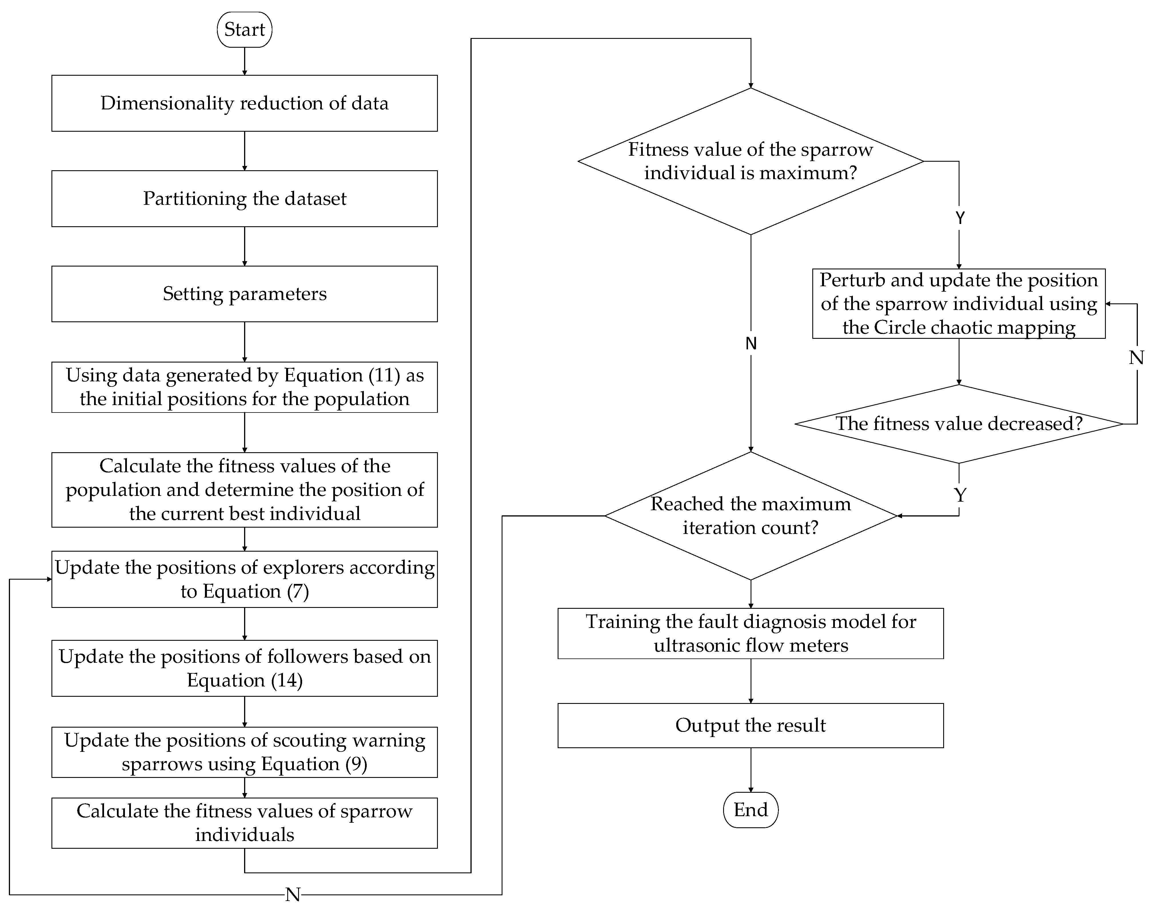
At present, there are few studies on the fault diagnosis of ultrasonic flow meters, and there is a problem of low diagnostic accuracy in the few studies that use data-driven methods for the fault diagnosis of ultrasonic flow meters. In response to the above issues, this article mainly diagnoses three types of faults in ultrasonic flow meters, namely gas intrusion, waxing, and installation effects. To address the issues of low fault-diagnosis accuracy and high feature dimensions caused by excessive interference information, we introduce a fault diagnosis algorithm utilizing KPCA-CLSSA-SVM. The structure of this paper is outlined as follows: Section 2 provides the theoretical framework, including an overview of the SVM model, an explanation of the basic principles of the sparrow search algorithm and its improved version, and a detailed elucidation of the proposed fault diagnosis algorithm’s basic workflow. Section 3 describes the database used in this study and provides a detailed overview of the experimental procedures. In Section 4, a rigorous evaluation of the model is conducted, including a comparison of feature distributions before and after processing and the fault diagnosis results obtained using different algorithms. Finally, Section 5 summarizes the research and concludes with key findings.

2. Fault Diagnosis Method Based on CLSSA-SVM

2.1. SVM Model

SVM is a classification algorithm that utilizes supervised learning to categorize data into two classes, with the aim of minimizing the structural risk. Its decision boundary is the maximum margin hyperplane obtained by solving the learning sample [19].

As shown in Figure 1, the solid-line plane is the required hyperplane, the dashed lines on both sides are the support planes, and the support vectors are the points on these two support planes. By scaling the values of $\omega$ and b in the expression, the distance between the obtained vector and the hyperplane is 1. The basic process of support vector machine classification is as follows:

• Set the regularization parameter C with a distance of $y_i=\omega x_i+\mathrm{b}$ and select the appropriate kernel function $K\left(x,z\right)$.

  $$\begin{array}{l}\underset{\mathsf{\zeta }}{\min }\frac{1}{2}{\displaystyle \sum _{i=1}^n{\displaystyle \sum _{j=1}^n{\mathsf{\zeta }}_i}}{\mathsf{\zeta }}_j{y}_i{y}_{j}K\left(x_i\cdot x_j\right)-{\displaystyle \sum _{i=1}^n{\mathsf{\zeta }}_i}\\ \begin{array}{cc}s.t.& \begin{array}{c}{\displaystyle \sum _{j=1}^n{\mathsf{\zeta }}_i{y}_i}=0\\ 0\le {\mathsf{\zeta }}_i\le C,i=1,2,\dots ,n\end{array}\end{array}\end{array},$$

  (1)
  We obtain the Lagrange multiplier ${\zeta }^{*}={\left({\zeta }_1^{*},{\zeta }_2^{*},\dots ,{\zeta }_n^{*}\right)}^T$.
• Calculate ${\omega }^{*}$.

  $${\omega }^{*}={\displaystyle \sum _{i=1}^n{\zeta }_i^{*}{y}_i{x}_i},$$

  (2)

Select a component ${\zeta }_j^{*}$ within a range of 0 to C in ${\zeta }_i^{*}$ and calculate ${\mathrm{b}}^{*}$.

$${\mathrm{b}}^{*}=y_j-{\displaystyle \sum _{i=1}^n{\mathsf{\zeta }}_j{y}_{i}K\left(x_i\cdot x_j\right)},$$

(3)

3.

Find the hyperplane and obtain the decision function:

$$f\left(x\right)=sign\left({\displaystyle \sum _{i=1}^n{\mathsf{\zeta }}_j{y}_{i}K\left(x_i\cdot x_j\right)}+{\mathrm{b}}^{*}\right),$$

(4)

4.

If the kernel function type is Gaussian, then $K\left(x,z\right)=\exp \left(-\frac{{\left|x-z\right|}^2}{g^2}\right)$.

According to the principle of the SVM, there are two parameters to be optimized in the classification model, namely the regularization parameter C and the kernel-function parameter g. These two parameter values are closely related to the anti-interference and generalization capabilities of the support vector machine. Therefore, we employ CLSSA to fine-tune the regularization parameters and kernel-function parameters, thereby enhancing the model’s accuracy and prediction performance.

Figure 1. Support vector machine classification model.

Figure 1. Support vector machine classification model.

2.2. Sparrow Search Algorithm (SSA)—Parameter Optimization of the SVM

SSA is a novel swarm-intelligence optimization method introduced by Xue [20] in 2020. Given a problem of dimension D, which represents the number of variables to be optimized, along with n being the number of sparrows and N representing the total sparrow count, the positions of the sparrows can be described as:

$$\begin{array}{cc}{X}_n=\left[x_{n,1},x_{n,2},\dots ,x_{n,D}\right]& n=1,2,3,\dots ,N,\end{array}$$

(5)

and the fitness of the sparrows can be described using the following matrix:

$$F_x=\left[\begin{array}{c}f\left(\left[x_{1,1},x_{1,2},\dots ,x_{1,D}\right]\right)\\ f\left(\left[x_{2,1},x_{1,2},\dots ,x_{2,D}\right]\right)\\ ⋮\\ f\left(\left[x_{n,1},x_{n,2},\dots ,x_{n,D}\right]\right)\end{array}\right],$$

(6)

where $f$ is the fitness value of the individual.

The equation for updating the position of explorers in the sparrow population is as follows:

$$X_{i,d}^{t+1}=\left\{\begin{array}{c}\begin{array}{cc}{X}_{i,d}^t\cdot \exp \left(-\frac{i}{\alpha \cdot \sigma }\right)& R_2\ge ST\end{array}\\ \begin{array}{cc}{X}_{i,d}^t+Q\cdot L& R_2\ge ST\end{array}\end{array}\right.,$$

(7)

The equation utilizes various parameters, including the current iteration count represented by t and the maximum iteration count denoted by $\sigma$. Additionally, it involves the position information of the i-th sparrow in the d-th dimension, denoted by $X_{i,d}$, and a random number $\alpha$. The variables R₂ and ST signify the alert and safety thresholds, respectively. Q is a random number following a normal distribution, and L represents a 1 × D matrix, where each element is 1. Notably, all sparrows in the population, except for the explorers, are considered followers. Followers adjust their positions based on Equation (8):

$$X_{i,d}^{t+1}=\left\{\begin{array}{c}\begin{array}{cc}Q\cdot \exp \left(-\frac{X_W-X_{i,d}^t}{i^2}\right)& i>\frac{n}{2}\end{array}\\ \begin{array}{cc}{X}_B^{t+1}+\left|X_{i,d}^t+X_B^{t+1}\right|\cdot A^T{\left(A{A}^T\right)}^{-1}\cdot L& otherwise\end{array}\end{array}\right.,$$

(8)

where $X_B$ denotes the optimal position of the explorers at present, while $X_W$ represents the current global worst position. A refers to a 1 × D matrix wherein each element receives a random assignment of either 1 or −1. Notably, sparrows designated for reconnaissance and early warning purposes constitute 10% to 20% of the total population, and the mathematical expression for their position update is as follows:

$$X_{i,d}^{t+1}=\left\{\begin{array}{c}\begin{array}{cc}{X}_B^t+\beta \cdot \left|X_{i,d}^t-X_W^t\right|& f_i>f_B\end{array}\\ \begin{array}{cc}{X}_{i,d}^t+R\cdot \frac{\left|X_{i,d}^t-X_W^t\right|}{\left(f_i-f_W\right)+\epsilon }& f_i=f_B\end{array}\end{array}\right.,$$

(9)

The parameter $\beta$, serving as a regulator for step size, is determined by a randomly generated number drawn from a normal distribution with the range of 0 to 1. R represents a randomly generated number within the range of −1 to 1, while $f_i$ signifies the fitness value of the current individual sparrow. Moreover, $f_B$ denotes the globally best fitness value observed at present, and $f_W$ represents the poorest fitness value. Meanwhile, ε is utilized as a minimal constant to prevent division by zero.

2.2.1. Circle Chaotic Mapping—Improving the Population Diversity

Chaos, characterized by its strong randomness and ergodicity, is a highly nonlinear natural phenomenon frequently utilized in optimization and search tasks. Presently, widely employed chaotic mappings encompass the tent, logistic, and circle chaotic mapping approaches [21,22]. Circle chaotic mapping, in addition to possessing strong stability, exhibits a high coverage of chaotic values. Therefore, this paper utilizes circle chaotic mapping to optimize the optimization algorithm.

Circular chaotic mapping is generally expressed mathematically as follows:

$$y_{i+1}=\mathrm{mod}(y_i+\chi -(\frac{\gamma }{2\pi })\sin (2\pi y_i),1),$$

(10)

In this paper, the values of $\chi$ and $\gamma$ are, respectively, 0.4204 and 0.0305.

The conventional sparrow search algorithm often encounters issues related to poor population diversity due to the random generation of initial positions for the sparrow population. This scenario results in a reduction of the algorithm’s convergence rate and precision. To address this, utilizing data generated by the circle chaotic mapping as the initial position information for the population proves effective. Perturbation and position updates are performed on the sparrows whose fitness values have not reached the maximum, thereby significantly enhancing the diversity of the search. The method of using data generated by the circle chaotic mapping to initialize the population’s positions can be described by Equation (11):

$$X_{i,d}=\kappa +(\mu -\kappa )\times y_i,$$

(11)

where $\kappa$ and $\mu$ respectively, provide the lowest and highest bounds of the entire search space.

2.2.2. Levy Flights—Enhancing Global Search Capabilities and Expediting Model Convergence

A Levy flight involves a point randomly moving in any direction within an arbitrary-dimensional space, traversing a random distance following a power-law distribution. This process can be repeated iteratively. The step-length distribution of Levy flights follows a heavy-tailed distribution, where each step direction is entirely random and of arbitrary length, while the distribution of step lengths follows a normal distribution. The exponential growth of step lengths imparts Levy flights with scale-invariant characteristics, which are widely applied in modeling classification problems [23,24,25].

The distance covered in a Levy flight can be defined as:

$$Levy(s)=0.01\times \delta \times \frac{u}{{\left|v\right|}^{1/\varsigma }},$$

(12)

where $\delta$ is a randomly generated number ranging from 0 to 1, $v~N\left(0,1\right)$, $u~N\left(0,\iota \right)$, and $\iota$ is obtained from Equation (13):

$$\iota =\left\{\frac{\mathrm{\Gamma }\left(1+\varsigma \right)\sin \left(\pi \varsigma /2\right)}{\mathrm{\Gamma }\left[\left(1+\varsigma \right)/2\right]\cdot \varsigma \cdot 2^{\left(\varsigma -1\right)/2}}\right\},$$

(13)

where $\mathrm{\Gamma }$ represents the gamma function, and $\varsigma$ takes a value of between 0 and 2, commonly chosen as 1.5.

After a certain number of iterations, when the fitness values of individual sparrows remain unchanged, followers turn into explorers. This situation often leads the algorithm becoming trapped in a local optimum. Hence, to minimize the likelihood of falling into local optima, Levy flights are introduced in the position update expression for the followers. The updated expression for the follower positions, after improvement, is as follows:

$$X_{i,d}^{t+1}=\left\{\begin{array}{ll}Q\cdot \exp (\frac{X_W-X_{i,d}^t}{i^2})\hfill & \hspace{1em}i>\frac{n}{2}\hfill \\ X_B^{t+1}\oplus Levy(s)\hfill & \hspace{1em}others\hfill \end{array}\right.,$$

(14)

2.3. A Modified Sparrow Search Algorithm

After integrating the two approaches described in Section 2.2.1 and Section 2.2.2, the proposed improved sparrow search algorithm operates through the following steps:

• Step 1: Define parameters including the iteration count, population size, ratio of explorers to followers, warning threshold, safety threshold, etc.
• Step 2: Utilize data generated by the circle chaotic mapping according to Equation (11) for initializing the population’s positions.
• Step 3: Compute the fitness values for the initial population and identify positions of the best and worst individuals in the current population.
• Step 4: Revise the positions of explorers according to Equation (7).
• Step 5: Revise the positions of followers according to Equation (14).
• Step 6: Update the positions of scouting warning sparrows using Equation (9).
• Step 7: Determine the positions and fitness values of each sparrow in space, sort them based on fitness values, and perturb and update the position of the sparrow possessing the highest fitness value using Equation (11).
• Step 8: If the maximum iteration count is reached, output the position information of the sparrow that has the best fitness value; otherwise, continue iterating.

2.4. Fault Diagnosis Process

Building upon the aforementioned discussion, we present a fault diagnosis model for ultrasonic flow meters utilizing an SVM enhanced by an improved optimization algorithm. The diagnostic algorithm follows these steps:

• Perform dimensionality reduction on the data from the ultrasonic flow meter.
• Initialize CLSSA parameters by setting the number of iterations, population size, ratio of explorers to followers, warning value, safety value, etc.
• Determine the range of regularization parameters and relevant parameters for the kernel function.
• Divide the dataset, reduced through kernel principal component analysis, into training and test sets at a ratio of 70:30. The fitness function, evaluated by RMSE between the predicted and actual values, aims to minimize disparities, seeking optimal solutions.
• Implement CLSSA iterations to converge toward the optimal solution for the two parameters until the maximum iteration count is reached.
• Output the optimal solution within the iteration count and employ the optimized parameters to train the SVM, thereby obtaining the fault diagnosis model for the ultrasonic flow meter.

The algorithm flowchart is depicted in Figure 2.

3. Experiments and Results

The ultrasonic flow meter is an instrument utilized for measuring fluid flow velocity. Its operational principle relies on the propagation of ultrasonic waves within the fluid medium. Typically, it incorporates a minimum of two transducers—one serving as a transmitter and the other as a receiver. These transducers are often positioned on opposing sides of the pipeline through which the fluid flows. The transmitter emits ultrasonic pulses, which propagate through the fluid to the receiver. The fluid flow exerts an influence on the propagation of ultrasonic waves, impacting the velocity, direction, and flow rate. Through the measurement of the ultrasonic wave propagation time and the received signal strength, the fluid flow velocity and flow rate can be derived.

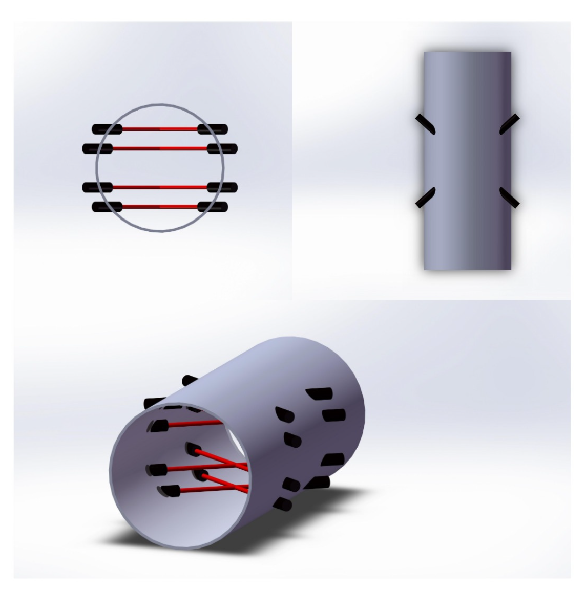
In the petroleum industry, liquid ultrasonic flow meters frequently encounter diverse faults during prolonged usage. The chemical nature of petroleum leads to wax deposition within the flow meter, while gases like methane in the pipeline also impact its functionality. Moreover, installation effects commonly contribute to errors in the practical application of ultrasonic flow meters. Due to the challenging setup of experimental platforms and limited research in related fields, the dataset used in this study is the publicly available UCI Ultrasonic Flow meter Fault Diagnosis Database collected by the University of Warwick, UK, and the National Engineering Laboratory. An 8-channel ultrasonic flow meter configuration, as shown in Figure 3, was used. The dataset comprises a total of 540 samples involving four types of flow meters [26].

Table 1. Information regarding the ultrasonic flow meter dataset.

Flow Meter	Samples	Channels	Feature Index	Features	Categories
A	87	8	1	Ratio of flatness	2
			2	Symmetricity
			3	Sideways flow
			4–11	Velocity along each of the eight channels
			12–19	Acoustic velocity in each of the eight channels
			20	Average acoustic velocity in all eight channels
			21–36	Amplification at either ends of each of the eight channels
B	92	4	1	Profile coefficient	3
			2	Symmetricity
			3	Sideways flow
			4	Swirl angle
			5–8	Velocity along each of the four channels
			9	Mean flow velocity across all four channels
			10–13	Acoustic velocity in four channels
			14	Average acoustic velocity in all four channels
			15–22	Signal intensity at each end of the four channels
			23–26	Flow disturbance in each of the four channels
			27	Meter performance
			28–35	Quality of signal at both ends of the four channels
			36–43	Amplification at both ends of the four channels
			44–51	Time for transit at both ends of the four channels
D‘	180	4	1	Profile coefficient	4
			2	Symmetricity
			3	Sideways flow
			4–7	Velocity along each of the four channels
			8–11	Acoustic velocity in the four channels
			12–19	Signal intensity at both ends of the four channels
			20–27	Quality of signal at both ends of the four channels
			28–35	Amplification at both ends of the four channels
			36–43	Time for transit at both ends of the four channels

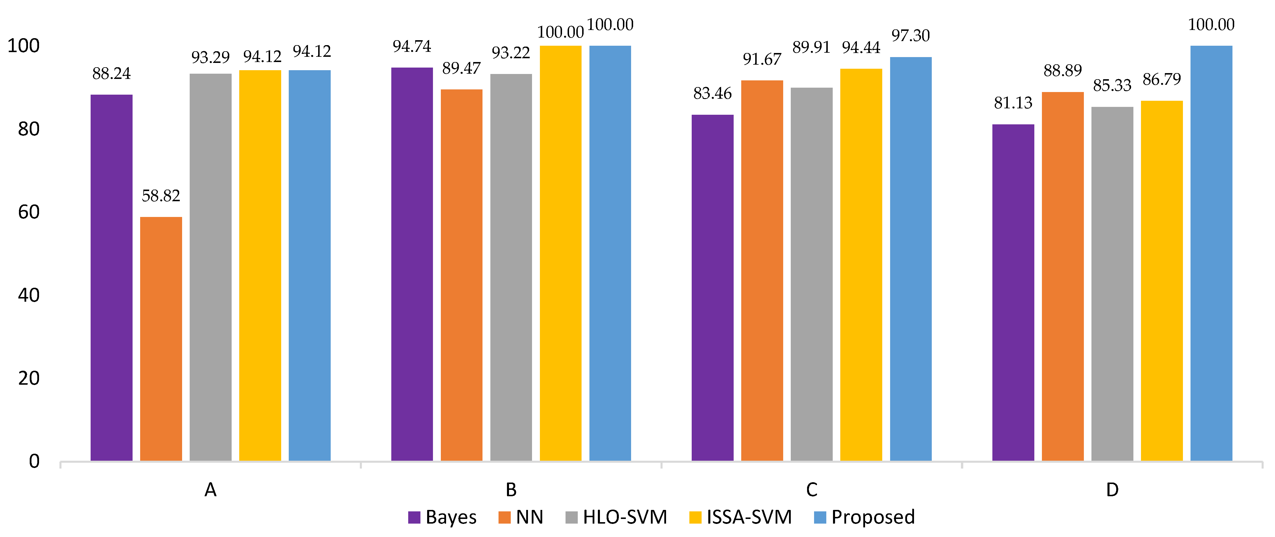
Due to the minor variation between flow meters C and D, with C having only one additional sample compared with D, the table does not delineate the C column.

presents basic information about the dataset, in which flow meter A has two types: normal and installation effects; flow meter B includes three types: normal, gas injection, and waxing; while flow meters C and D encompass four types: normal, gas injection, waxing, and installation effects.

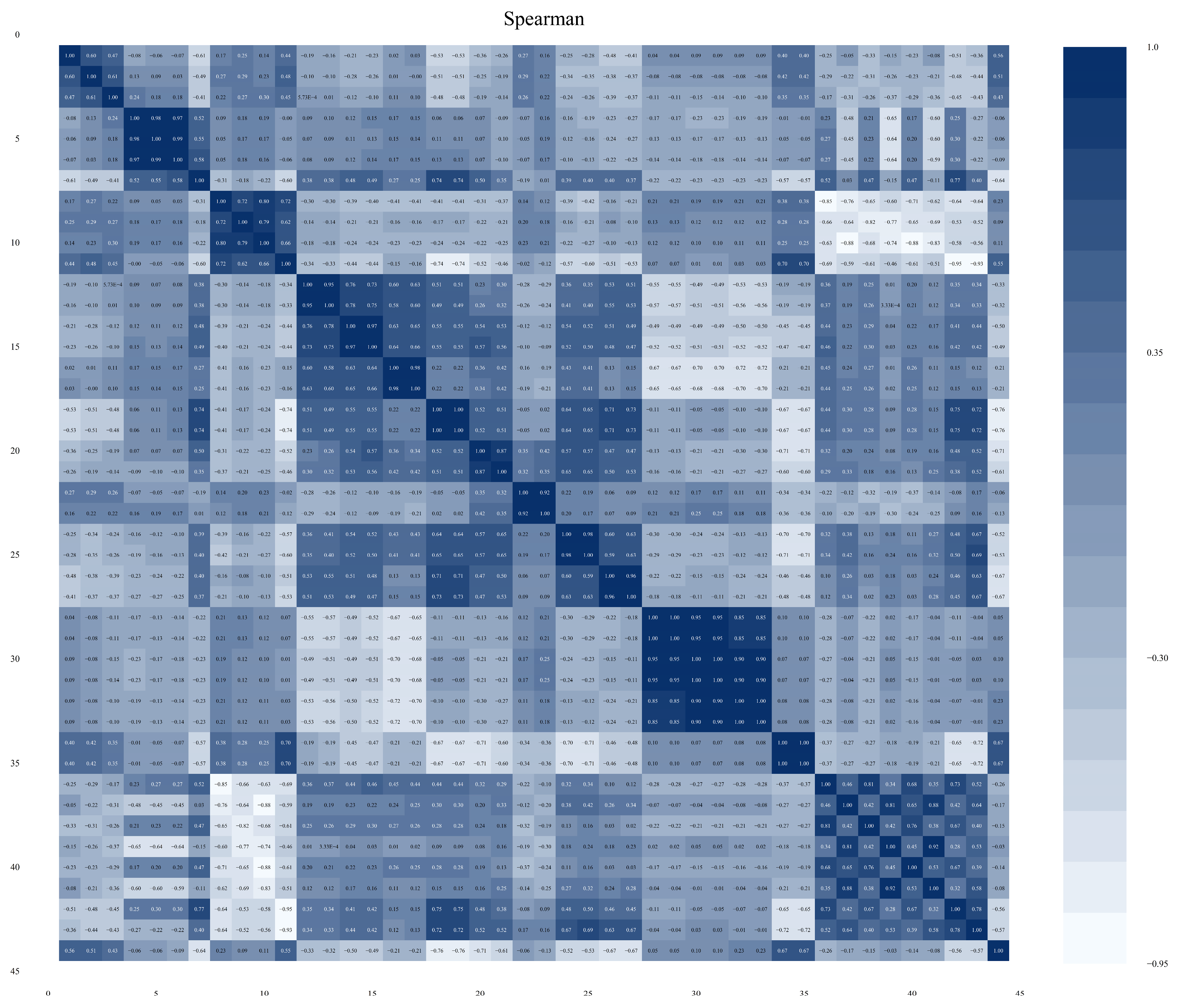
3.1. Data Correlation Analysis

Due to the numerous diagnostic parameters of the flow meter, there might be interdependencies among the collected data. Therefore, it is essential to perform a correlation analysis on the collected data. Since the Pearson correlation coefficient lacks sensitivity to nonlinear relationships and may not precisely represent the correlation between features, the Spearman correlation coefficient is employed to capture the correlation between features. The formula for calculating the Spearman correlation coefficient is as follows:

$$\rho =\frac{{\displaystyle {\sum }_i\left(x_i-\overline{x}\right)}\left(y_i-\overline{y}\right)}{\sqrt{{\displaystyle {\sum }_i{\left(x_i-\overline{x}\right)}^2}{\displaystyle {\sum }_i{\left(y_i-\overline{y}\right)}^2}}},$$

(15)

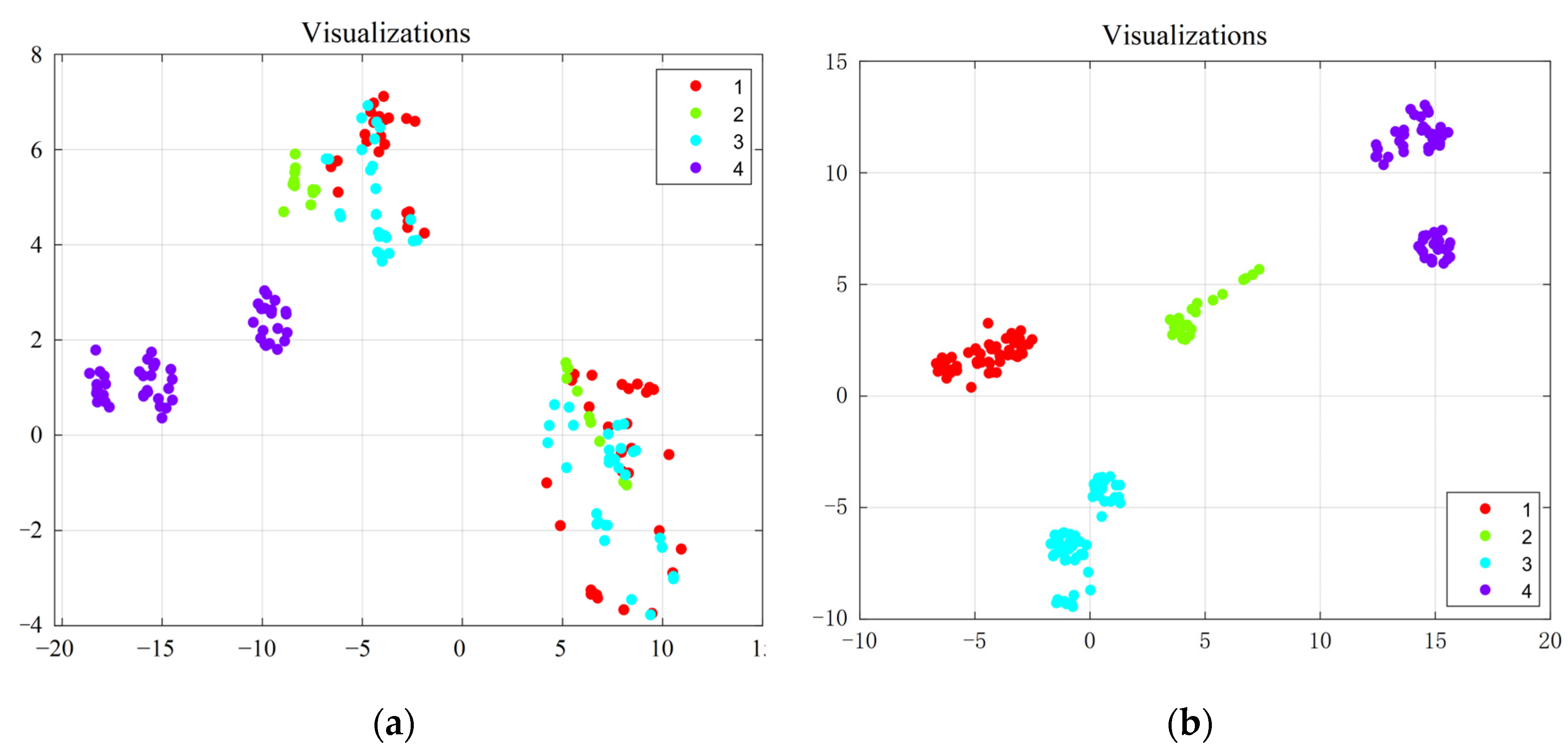
in which $\rho >0$ indicates a positive correlation between two features, and $\rho <0$ signifies a negative correlation between them. Taking flow meter D as an example, an analysis of the Spearman correlation coefficients for diagnostic parameters is performed. As shown in Figure 4, there are notably high correlations between the flow rates of the first, second, and third channels between the sound velocities of the four channels and between the gains at both ends of the channels, as well as between the flight time and the sound velocity. Therefore, it is essential to employ a correlation-based dimensionality reduction algorithm to eliminate highly correlated features to prevent the potential overfitting of the algorithm, and thereby avoiding a reduction in the model accuracy.

3.2. Data Preprocessing

As per Section 3.1, although the dataset constructed from the ultrasonic flow meter fault-diagnosis database does not contain any missing data, there are high correlations among many features. Due to the high dimensionality of features, which can lead to computational complexities, it is essential to reduce the dimensionality using kernel principal component analysis (KPCA). The calculation method is as follows [27]:

The dataset is denoted as $\mathit{S}={[S_1\hspace{1em}{S}_2\hspace{1em}{S}_3\hspace{1em}\cdots \hspace{1em}{S}_n]}^T$, where $S_i$ represents a collection of m data points for each feature, and n denotes the number of feature types. Initially, S will be mapped to a high-dimensional space:

$$\Phi =K(S_i,S_j)=\left(\begin{array}{ccc}\varphi (x_{11})& \cdots & \varphi (x_{1m})\\ ⋮& \ddots & ⋮\\ \varphi (x_{n1})& \cdots & \varphi (x_{nm})\end{array}\right),$$

(16)

where $\varphi$ is a nonlinear mapping function. $\Phi$ is centralized to obtain ${\Phi }^{’}$; then, the covariance matrix G is calculated. The eigenvalues of E are computed and arranged in descending order, denoted as ${\lambda }_1,{\lambda }_2,{\lambda }_3,\dots ,{\lambda }_n$, along with the corresponding eigenvectors $o_1,o_2,o_3,\dots ,o_n$. Defining the eigenvector matrix as $P=\left[o_1,o_2,o_3,\dots ,o_n\right]$, $PG{P}^T$ is represented as:

$$PG{P}^T=\left(\begin{array}{cccc}{\lambda }_1& 0& \cdots & 0\\ 0& {\lambda }_2& \cdots & 0\\ ⋮& ⋮& \ddots & ⋮\\ 0& 0& \cdots & {\lambda }_n\end{array}\right),$$

(17)

Finally, taking the first k columns of $PG{P}^T$ to form a new matrix $Q=\left[o_1,o_2,o_3,\dots ,o_k\right]$, we obtain the reduced principal-component-dataset matrix Z:

$$\mathit{Z}=\mathit{Q}\Phi ,$$

(18)

In the feature space, all sample features have an equal influence on distance, but due to varying value ranges, certain feature values dominate the distances between sample points. To tackle this problem, this paper employs a normalization approach, mapping the data after dimensionality reduction to the range [0, 1].

3.3. Model Determination Experiment of Ultrasonic Flow Meter Fault Diagnosis Based on KPCA-CLSSA-SVM

This paper presents a fault diagnosis algorithm for ultrasonic flow meters by utilizing KPCA-CLSSA-SVM. The algorithm takes parameter features collected from ultrasonic flow meters as input and outputs the type of fault detected in the flow meter.

Using the MATLAB R2019a framework within the libsvm environment, we constructed the fault diagnosis model using KPCA-CLSSA-SVM. To validate the model’s effectiveness, a series of experiments were conducted. The input for the model consists of the aforementioned parameter features, with a size of (Num, Fea). Here, Num represents the sample count for this type of flow meter, while Fea denotes the collected features specific to this flow meter.

The suitability of model parameters determines the excellence of the model’s performance. For the D-type flow meter, experiments were conducted to determine the superiority of the model’s related parameters. Parameters adjusted in the experiments include the kernel-function type for the kernel principal component analysis, the dimensionality of the dataset after dimensionality reduction, the population count of sparrows, the number of iterations for the improved sparrow search algorithm, the kernel-function type, and certain parameters within the kernel function for support vector machines. Ten experiments were conducted for each parameter value, and the average of these ten experimental results was used as the evaluation criterion [10].

The role of a kernel is to convert the original data into a higher-dimensional space. Different kernel functions perform different transformations on the data, thereby affecting the efficacy of dimensionality reduction. For instance, the commonly used Gaussian kernel function can map data into an infinite-dimensional space, but it typically has a slower computation speed. Conversely, the linear kernel function, often chosen as the primary option, possesses strong interpretability and simplicity in computation but lacks the ability to address nonlinear problems.

To determine the required kernel function for this method, the experimental settings were as follows: the kernel-function types for the kernel principal component analysis were set as polynomial, linear, and Gaussian kernel functions. The dimensionality of the dataset after dimensionality reduction was set to 15. The population count of sparrows was set to 8, the number of iterations for the improved sparrow search algorithm was set to 30, and the type of support vector machine was set as C-SVC, with the kernel-function type set as a linear kernel function. By analyzing the impact of different kernel-function types in the kernel principal component analysis of model performance, the final choice of kernel-function type was determined.

As shown in

Table 2. The impact of different kernel-function types in KPCA on the model.

Types	Polynomial	Linear	Gaussian
Accuracy (%)	79.56	73.89	75.95

, when the polynomial kernel-function type was selected, the accuracy reached its highest point. Therefore, the polynomial kernel function was chosen for the kernel principal component analysis.

Once the kernel function for the KPCA was determined, further experiments were conducted to select the dimensionality of the dataset after dimensionality reduction. A too-low dimensionality could lead to loss of feature information, making classification more challenging. Conversely, an excessively high dimensionality would increase the computational complexity and potentially lead to overfitting of the model. Using the linear kernel function, the dataset dimensionality after dimensionality reduction was set to 11, 18, 25, and 32. As indicated in

Table 3. The impact of dataset dimensionality after dimensionality reduction on the model.

Dimensionality	11	18	25	32
Accuracy (%)	79.62	80.75	85.17	79.25

, when the dimensionality of the dataset after dimensionality reduction was set to 25, the accuracy reached its peak. Therefore, the dataset’s dimensionality after dimensionality reduction was set to 25.

Next, further experiments were conducted on the population count of sparrows. The population count of sparrows was set to 20, 30, 40, and 50. As shown in

Table 4. The impact of the population counts of sparrows on the model.

Population	20	30	40	50
Accuracy (%)	86.41	87.60	88.28	88.51

, with an increase in the population count of sparrows, the model’s accuracy improved. The accuracy of the model tended to stabilize when the population count reached 40. However, excessively high population counts could increase algorithmic complexity. Therefore, in this model, the population count of sparrows was set to 30.

Then, experiments were conducted on the number of iterations for the algorithm. The number of iterations for the algorithm was set to 40, 50, 60, and 70. As shown in

Table 5. The effect of the iteration counts for the enhanced SSA on the model.

Iterations	40	50	60	70
Accuracy (%)	79.62	80.75	85.17	79.25

, after reaching 60 iterations, the accuracy of the model tended to stabilize. However, too many iterations could decrease the training speed of the model. Consequently, in this context, the iteration count for the enhanced sparrow search algorithm was established at 50.

After the parameter settings for the data dimensionality reduction algorithm and optimization algorithm were completed, we proceeded to configure some parameters for the support vector machine. Due to the various fault types in ultrasonic flow meters, we selected a multi-classification support vector machine; specifically, C-SVC. The kernel function in SVM significantly influences its classification performance. In this study, experiments were conducted using different kernel functions: linear, polynomial, Gaussian, and sigmoid. The results are presented in

Table 6. The impact of different kernel-function types in support vector machines on the model.

Types	Linear	Polynomial	Gaussian	Sigmoid
Accuracy (%)	92.86	97.30	83.78	29.73

. When employing the sigmoid kernel function, the SVM exhibits a functionality similar to that of a multi-layer neural network. However, its relatively lower accuracy suggests that neural network algorithms might not be suitable for diagnosing faults in ultrasonic flow meters.

Finally, after deciding on the use of the polynomial kernel function for the support vector machine, we needed to set certain parameters for the polynomial kernel function; specifically, the highest degree of the polynomial. In libsvm, the highest degree of the polynomial is denoted by the parameter “degree”. As shown in

Table 7. The impact of different highest degrees in polynomial kernel functions on the model.

Degree	1	2	3	4
Accuracy (%)	90.16	94.67	100.00	95.13

, when the highest degree is less than 3, the model’s accuracy is positively correlated with the highest degree. This indicates that the linear kernel function and the quadratic polynomial kernel function fail to meet the fitting requirements, and increasing the highest degree of the polynomial kernel function can improve the model’s accuracy. However, when the highest degree is greater than 3, the model’s accuracy is negatively correlated with the highest degree. This is because higher degrees may lead the model to overfit, decreasing its accuracy. When the “degree” is set to 3, indicating a third-degree polynomial kernel function, the model achieves the highest accuracy. Therefore, the highest degree of the polynomial kernel function in this paper was set to 3.

3.4. The Experimental Results

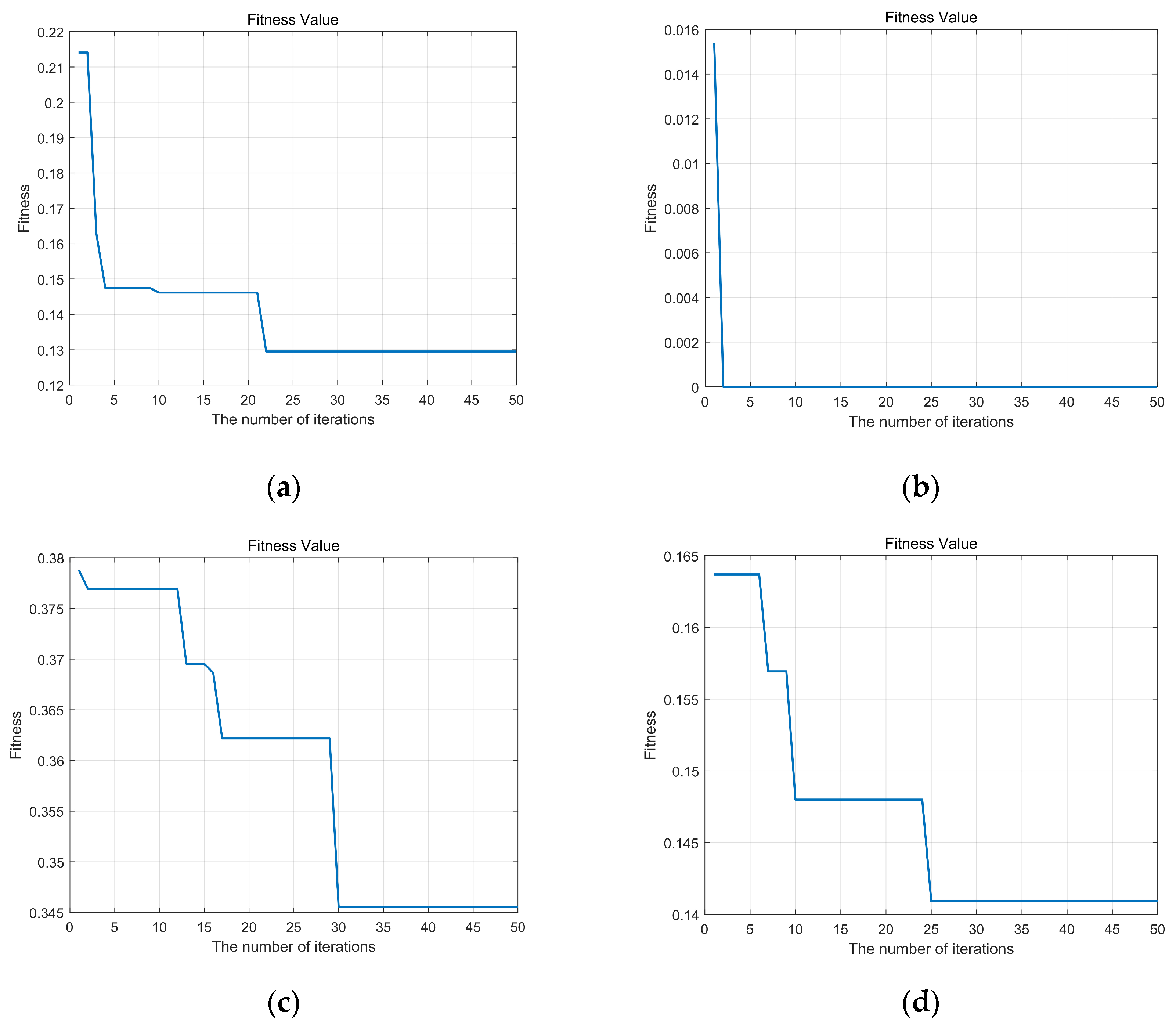
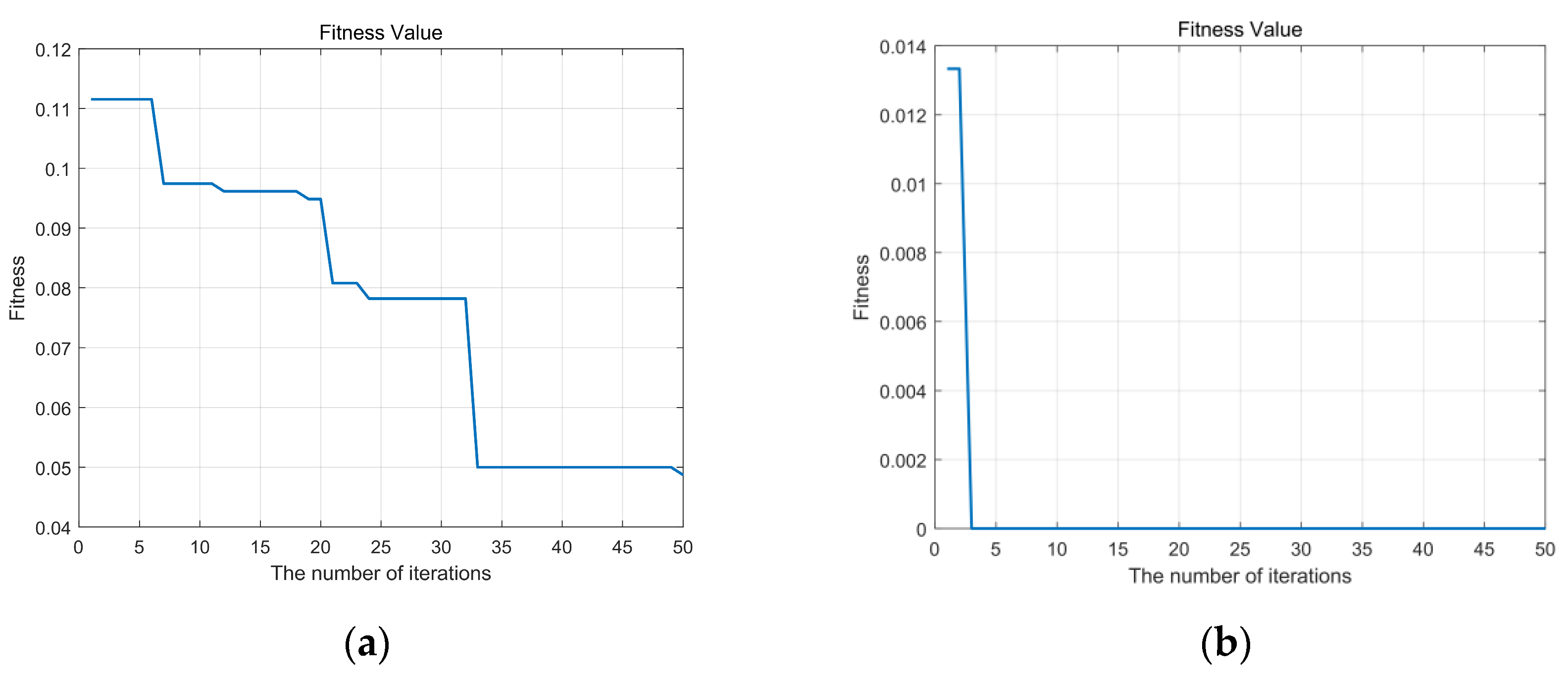
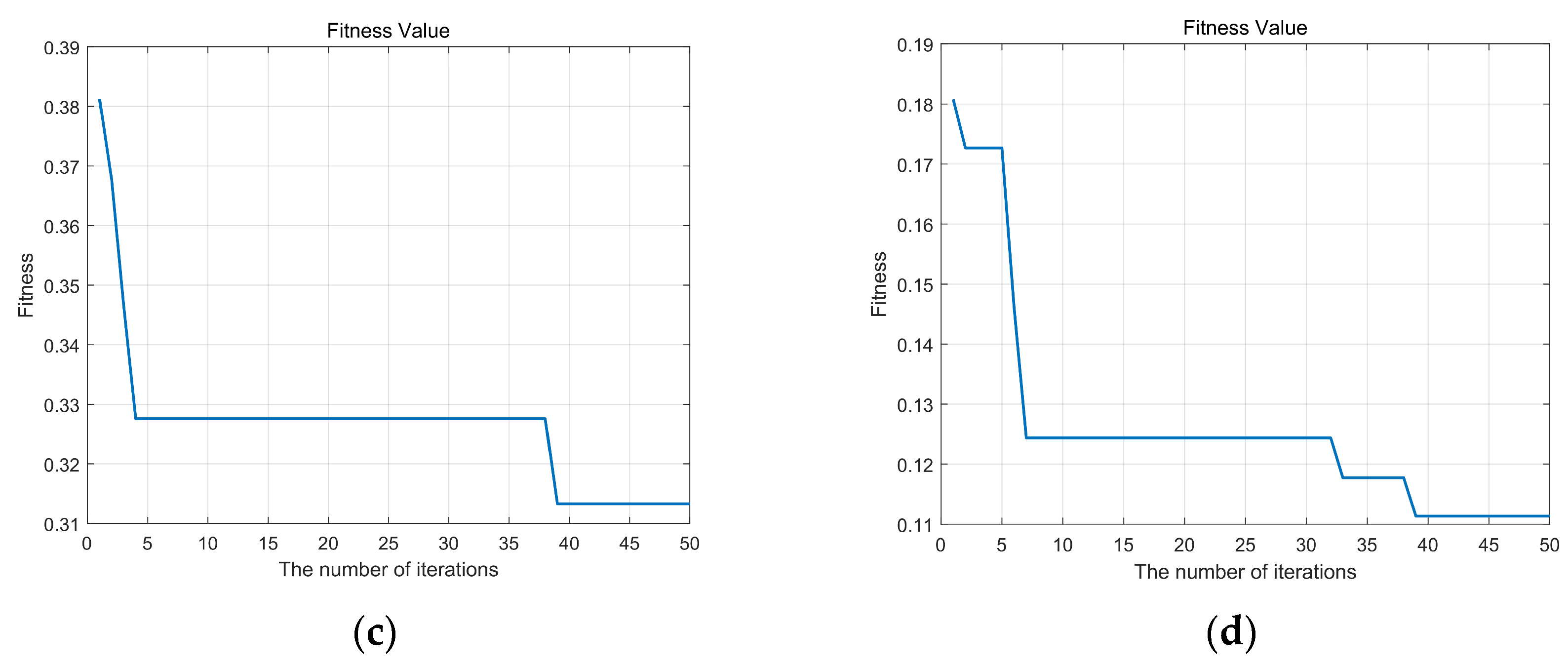
After determining the model parameters, the collected data was fed into the fault diagnosis model. Approximately 80% of the data was used for training, while the other 20% was set aside for testing. Figure 5 and Figure 6 display the curves depicting the changes in fitness values with iterations for the sparrow search algorithm, both before and after improvements. Lower fitness values indicate a decreased probability of the algorithm becoming stuck in local optima. Comparing these two sets of graphs, noticeable enhancements are observed in the performance of flow meters A, C, and D, while flow meter B demonstrates relatively minor improvements. This is attributed to the higher dimensionality of the dataset associated with flow meter B, indicating strong separability among its data, thus requiring no algorithmic improvements to achieve optimal parameters with high accuracy.

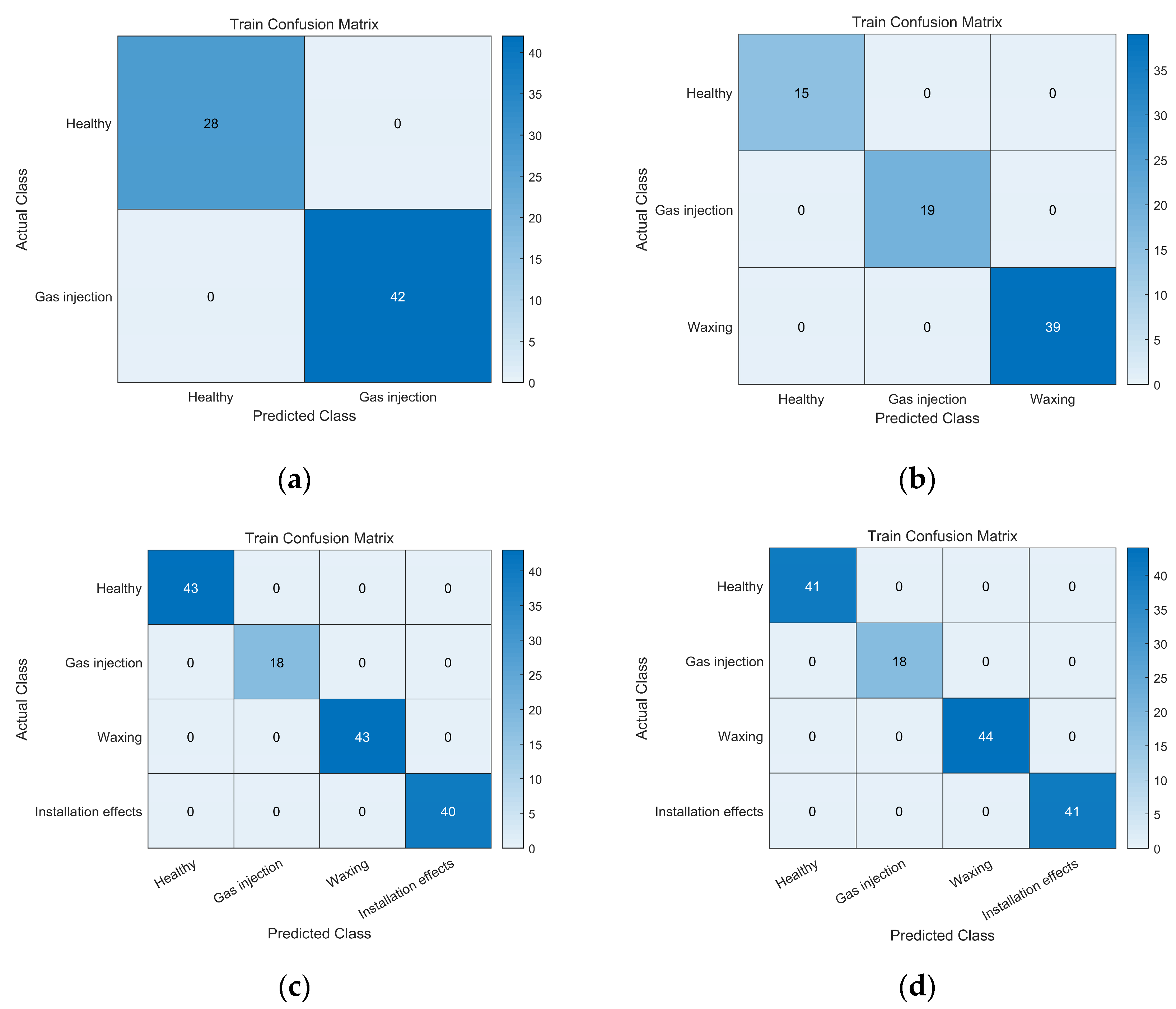
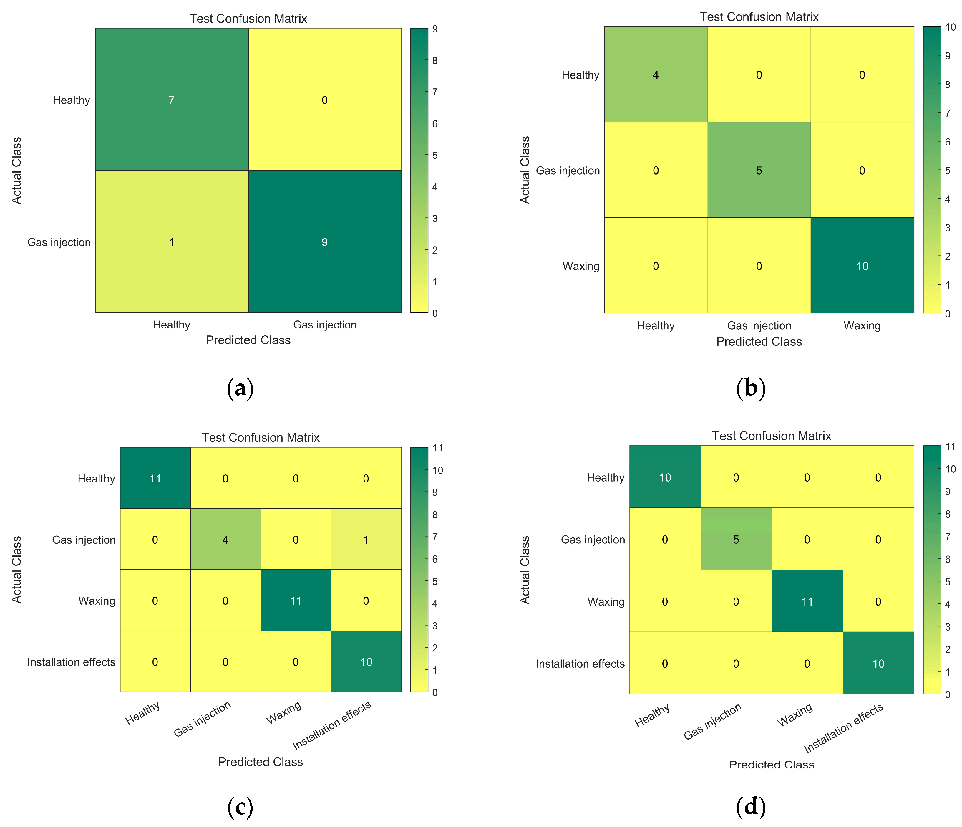
In this part, we will also utilize a confusion matrix as a measure to evaluate the precision of the fault diagnosis model. The confusion matrix measures the model’s classification performance by calculating the number of correct and incorrect classifications. Figure 7 represents the confusion matrices of the prediction results for the training set of the four types of flow meters, and Figure 8 represents the confusion matrices of the prediction results for the test set of the four types of flow meters. The horizontal axis shows the model’s predictions, while the vertical axis represents the fault categories. It is evident that this algorithm yields favorable classification results for both the test and training sets.

4. Evaluation and Discussion

4.1. Performance Evaluation of Model Feature Extraction

To evaluate the effectiveness of the features extracted by the model, this study utilized LargeVis for an intuitive analysis of the collected raw data and the data computed by the algorithm. LargeVis is a relatively novel dimensionality reduction algorithm proposed by Tang et al. [28]. In comparison with the commonly used t-SNE, LargeVis employs optimization techniques such as random projection trees and negative sampling, significantly reducing the time complexity. We employed LargeVis to map the data into two dimensions, plot a scatter plot, and assess the effectiveness of the extracted features. The visualization results are depicted in Figure 9. It can be observed that the raw, untreated data exhibit significant overlap. However, after feature extraction through the algorithm, the four categories are completely separable. Thus, this model demonstrates strong capabilities in extracting fault features specific to ultrasonic flow meters.

4.2. Comparative Analysis of Diagnostic Performance among Different Models

To validate the algorithm’s performance, the proposed fault diagnosis method was compared with those based on Bayes, NN, HLO-SVM, and ISSA-SVM. As illustrated in Figure 10, for diagnosing faults in flow meters A and B, the differences in performance among the four algorithms were minimal. When diagnosing faults in flow meters C and D, the performance differences among the four algorithms varied. In particular, the SVM algorithm exhibited a prediction accuracy of below 85%. Conversely, KPCA-CLSSA-SVM achieved a prediction accuracy of over 94% for all the types of flow meters, consistently outperforming the other algorithms.

The algorithm proposed in this paper shows higher predictive accuracy compared with other algorithms, as observed in Figure 10. Several reasons can be attributed to this higher accuracy. Initially, the algorithm utilizes KPCA to decrease the dimensionality of the gathered raw data. This process eliminates highly correlated features, reducing model complexity while minimizing the impact of irrelevant information on predictive accuracy. Secondly, it utilizes data generated by circle chaotic mapping as the initial position information for the population, perturbing and updating the positions of sparrows whose fitness values have not reached their maximum. Furthermore, it improves the position update expression for the sparrow followers by employing Levy flights, enhancing the global search capability of the SSA without compromising search speed, thus ensuring the capability to optimize. Lastly, the CLSSA algorithm is used to find the relevant parameters for the SVM, preventing the issue of lower accuracy resulting from solely relying on the empirical selection of SVM parameters.

5. Conclusions

During transportation and usage, ultrasonic flow meters often encounter various malfunctions. Failure to promptly detect these issues can disrupt trade fairness and, in severe cases, compromise personnel safety. Traditional malfunction detection methods are relatively slow, involve numerous factors, and demand a higher skill level from the inspectors. This article’s approach is data-driven, and its key innovations are summarized as follows:

• The study introduced a comprehensive fault diagnosis approach. The flow data collected inside the pipeline and the features of the flow meter itself can be directly input into the fault diagnosis model. Simultaneously, an attention mechanism has been integrated, allowing the real-time remote acquisition of fault diagnosis results of ultrasonic flow meters under external environmental interference.
• This paper improved the classification performance of the SVM using an improved sparrow search algorithm. This improved algorithm was employed to seek parameters that optimize the performance of the SVM. In contrast with traditional methods that rely on empirical parameter selections for the SVM, this approach has the potential to enhance model accuracy.
• The study introduced circle chaotic mapping to increase the variation within the sparrow population. Circle chaotic mapping exhibits strong stability and a high chaotic-value coverage rate. Utilizing data generated by the circle chaotic mapping as the initial position information for the population, and perturbing and updating the positions of sparrows whose fitness values have reached their maximum, the variation in the search was effectively increased. Additionally, to avoid the sparrow search algorithm from becoming trapped in local optima, a Levy flight was introduced. Each step direction of a Levy flight is entirely random, with a length following a normal distribution and a variable step size. Improvements in the update expression for the positions of sparrow followers using Levy flights enhance the global search capability and convergence speed while maintaining optimization speed.

Finally, this study conducted experiments on four types of ultrasonic flow meters using features such as the profile coefficient, flow rate, and signal-to-noise ratio, among others, as experimental data. These were utilized for training and testing the model, achieving fault diagnosis for the ultrasonic flow meters. The experimental results indicate that the fault diagnosis predictive models built for the four flow meters using this algorithm had prediction accuracies of over 94%, surpassing the overall diagnostic performance of other algorithms. Hence, the ultrasonic flow meter fault-diagnosis method based on KPCA-CLSSA-SVM has been proved to be a promising solution within the field of ultrasonic flow meter fault diagnosis.

References

1. Chen, X.; Li, J.; Cheng, H.; Li, B.; He, Z. Research and Application of Condition Monitoring and Fault Diagnosis Technology in Wind Turbines. J. Mech. Eng. 2011, 47, 45–52. [Google Scholar] [CrossRef]
2. Hao, R.; Lu, W.; Chu, F. Review of Diagnosis of Rolling Element Bearings Defaults by Means of Acoustic Emission Technique. J. Vib. Shock 2008, 27, 75–79+181. [Google Scholar]
3. Ding, J.; Yang, X.; Chu, X. Research on vibration monitoring and fault diagnosis of large pumping station units. Pump Technol. 2004, 2, 41–43. [Google Scholar]
4. Liu, P.; Wang, L.; Zhang, C.; Zheng, D. Research status and development trend of condition monitoring on main-shaft bearings used in aircraft engines. J. Aerosp. Power 2022, 37, 330–343. [Google Scholar]
5. Aziz, S.; Khan, M.; Faraz, M.; Montes, G. Intelligent bearing faults diagnosis featuring Automated Relative Energy based Empirical Mode Decomposition and novel Cepstral Autoregressive features. Measurement 2023, 216, 112871. [Google Scholar] [CrossRef]
6. Jaramillo, F.; Gutiérrez, J.; Orchard, M.; Guarini, M.; Astroza, R. A Bayesian approach for fatigue damage diagnosis and prognosis of wind turbine blades. Mech. Syst. Signal Process. 2022, 174, 109067. [Google Scholar] [CrossRef]
7. Gyamfi, K.; Brusey, J.; Hunt, A.; Gaura, E. Linear dimensionality reduction for classification via a sequential Bayes error minimisation with an application to flow meter diagnostics. Expert Syst. Appl. 2018, 91, 252–262. [Google Scholar] [CrossRef]
8. Tan, Q.; Mu, X.; Fu, M.; Yuan, H.; Sun, J.; Liang, G.; Sun, L. A new sensor fault diagnosis method for gas leakage monitoring based on the naive Bayes and probabilistic neural network classifier. Measurement 2022, 194, 111037. [Google Scholar] [CrossRef]
9. Silva, P.; Gabbar, H.; Junior, P.; Junior, C. A new methodology for multiple incipient fault diagnosis in transmission lines using QTA and Naïve Bayes classifier. Int. J. Electr. Power Energy Syst. 2018, 103, 326–346. [Google Scholar] [CrossRef]
10. Zhu, J.; Lü, B.; Qiao, S.; Wang, Y.; Chen, J. Application of Primary Component Analysis and Multivariate Gaussian Bayesian Method on Intelligent Failure Diagnosis of Ultrasonic Flowmeter. Acta Metrol. Sin. 2020, 12, 1494–1499. [Google Scholar]
11. Li, H.; Zhang, Q.; Qin, X.; Sun, Y. Fault diagnosis method for rolling bearings based on short-time Fourier transform and convolution neural network. J. Vib. Shock 2018, 19, 124–131. [Google Scholar]
12. Al-Wahaibi, S.; Abiola, S.; Chowdhury, M.; Lu, Q. Improving convolutional neural networks for fault diagnosis in chemical processes by incorporating global correlations. Comput. Chem. Eng. 2023, 176, 108289. [Google Scholar] [CrossRef]
13. Abdelmaksoud, M.; Torki, M.; El-Habrouk, M.; Elgeneidy, M. Convolutional-neural-network-based multi-signals fault diagnosis of induction motor using single and multi-channels datasets. Alex. Eng. J. 2023, 73, 231–248. [Google Scholar] [CrossRef]
14. Vapnik, V. Bounds on the Rate of Convergence of Learning Processes. In The Nature of Statistical Learning Theory; Springer: New York, NY, USA, 2000; pp. 69–91. [Google Scholar]
15. Chatterjee, S.; Gatla, R.; Sinha, P.; Jena, C.; Kundu, S.; Panda, B.; Nanda, L.; Pradhan, A. Fault detection of a Li-ion battery using SVM based machine learning and unscented Kalman filter. Mater. Today Proc. 2023, 74, 703–707. [Google Scholar] [CrossRef]
16. Huang, X.; Teng, Z.; Tang, Q.; Yu, Z.; Hua, J.; Wang, X. Fault diagnosis of automobile power seat with acoustic analysis and retrained SVM based on smartphone. Measurement 2022, 202, 111699. [Google Scholar] [CrossRef]
17. Sarita, K.; Kumar, S.; Saket, R. OC fault diagnosis of multilevel inverter using SVM technique and detection algorithm. Comput. Electr. Eng. 2021, 96, 107481. [Google Scholar] [CrossRef]
18. Zhang, Q.; Yao, J. Research on Fault Diagnosis Method of Ultrasonic Flowmeter Based on hybrid Kernel SVM Algorithm. In Proceedings of the 40th China Control Conference, Shanghai, China, 26–28 July 2021. [Google Scholar]
19. Lin, Q. Plate Recognition System Based on SVM and ANN Neural Network. Software 2019, 8, 105–107. [Google Scholar]
20. Xue, J.; Shen, B. A novel swarm intelligence optimization approach: Sparrow search algorithm. Syst. Sci. Control Eng. 2020, 8, 22–34. [Google Scholar] [CrossRef]
21. Wu, R.; Huang, H.; Wei, J.; Ma, C.; Zhu, Y.; Chen, Y.; Fan, Q. An improved sparrow search algorithm based on quantum computations and multi-strategy enhancement. Expert Syst. Appl. 2023, 215, 119421. [Google Scholar] [CrossRef]
22. Huang, J. Research on Sparrow Search Algorithm Based on Fusion of T Distribution and Tent Chaotic Mapping. Master’s Thesis, Lanzhou University, Lanzhou, China, 2021. [Google Scholar]
23. Zhang, Y.; Qin, L. Improved Salp Swarm Algorithm Based on Levy Flight Strategy. Comput. Sci. 2020, 47, 154–160. [Google Scholar]
24. Wang, Z.; Chen, Y.; Ding, S.; Liang, D.; He, H. A novelparticle swarm optimization algorithm with Lévy flight and orthogonal learning. Swarm Evol. Comput. 2022, 75, 101207. [Google Scholar] [CrossRef]
25. Jensi, R.; Jiji, W. An enhanced particle swarm optimization with levy flight for global optimization. Appl. Soft Comput. 2016, 43, 248–261. [Google Scholar] [CrossRef]
26. Ultrasonic Flowmeter Diagnostics. UCI Machine Learning Repository. Available online: https://archive.ics.uci.edu/dataset/433/ultrasonic+flowmeter+diagnostics (accessed on 16 May 2023).
27. Yang, J.; Frangi, A.; Yang, J.; Zhang, D.; Jin, Z. KPCA plus LDA: A complete kernel Fisher discriminant framework for feature extraction and recognition. IEEE Trans. Pattern Anal. Mach. Intell. 2015, 27, 230–244. [Google Scholar] [CrossRef] [PubMed]
28. Tang, J.; Liu, Z.; Zhang, M.; Mei, Q. Visualizing Large-scale and High-dimensional Data. In Proceedings of the 25th International Conference on World Wide Web—WWW’16, Montréal, QC, Canada, 11–15 April 2016. [Google Scholar]
Figure 2. Flowchart of the proposed diagnostic algorithm for ultrasonic flow meters.
Processes 12 00809 g002
Figure 3. The configuration of the 8-channel ultrasonic flow meter.
Processes 12 00809 g003
Figure 4. The Spearman correlation coefficient heatmap for diagnostic parameters of flow meter D.
Processes 12 00809 g004
Figure 5. The fitness-value curves for the four types of flow meters using the unimproved algorithm are as follows: (a) Type A; (b) Type B; (c) Type C; (d) Type D.
Processes 12 00809 g005
Figure 6. The fitness-value curves for the four types of flow meters using the improved algorithm are as follows: (a) Type A; (b) Type B; (c) Type C; (d) Type D.
Processes 12 00809 g006aProcesses 12 00809 g006b
Figure 7. Confusion matrices for the predicted results of the four types of flow meters in the training set: (a) Type A; (b) Type B; (c) Type C; (d) Type D.
Processes 12 00809 g007
Figure 8. Confusion matrices for the predicted results of the four types of flow meters in the test set: (a) Type A; (b) Type B; (c) Type C; (d) Type D.
Processes 12 00809 g008
Figure 9. Feature visualization comparison: (a) feature visualization of the raw data; (b) feature visualization of the data after algorithm processing.
Processes 12 00809 g009
Figure 10. Comparative predictive accuracy of fault diagnosis models.
Processes 12 00809 g010