Rapid Classification and Diagnosis of Gas Wells Driven by Production Data

Abstract

Conventional gas well classification methods cannot provide effective support for gas well routine management, and suffer from poor timeliness. In order to guide the on-site operation in liquid loading gas wells and improve the timeliness of gas well classification, this paper proposes a production data-driven gas well classification method based on the LDA-DA (Linear Discriminant Analysis–Discriminant Analysis) combination model. In this method, considering the requirements of routine management, gas wells are evaluated from two aspects: liquid drainage capacity (LDC) and liquid production intensity (LPI), and are classified into six types. Domain knowledge is used to perform the feature engineering on the on-site production data, and five features are set up to quantitatively evaluate the gas well and to create classification samples. On this basis, in order to specify the optimal data processing flow to establish the gas well classification map, four linear dimensionality reduction techniques, LDA, PCA, LPP, and ICA, are used to reduce the dimensionality of original classification samples, and then, four classical classification algorithms, NB, DA, KNN, and SVM, are trained and evaluated on the low-dimensional samples, respectively. The results show that the LDA space achieves the optimal sample separation and is chosen as the decision space for gas well classification. The DA algorithm obtains the top performance, i.e., the highest Average Macro F1-score of 95.619%, in the chosen decision space, and is employed to determine the classification boundaries in the decision space. At this point, the LDA-DA combination model for sample data processing is developed. Based on this model, gas well classification maps can be established by data mining, and the rapid evaluation and diagnosis of gas wells can be achieved. This method realizes instant and efficient production data-driven gas well classification, and can provide timely decision-making support for gas well routine management. It introduces new ideas for performing gas well classification, expanding the content and scope of the classification work, and presenting valuable insights for further research in this field.

1. Introduction

In mature gas reservoirs, the gas–liquid contradiction becomes prominent and the overall liquid production remains stubbornly high. There are a large number of low-pressure wells and liquid-producing wells on site, bringing great challenges to the production management of gas wells [1]. In order to summarize production practices and improve management efficiency, gas well classification is generally implemented in on-site management. Gas wells with the same production characteristics are classified into one category, and a comprehensive analysis of these wells is conducted to reveal their common production laws [2]. Through classification work, field operators can quickly grasp the production characteristics of gas wells, master their production status, and subsequently formulate targeted management strategies in time, so as to ensure the optimal production of gas wells and improve the overall development effect of gas reservoirs [1].

Analyzing the production status and then predicting and treating the liquid loading is a significant portion of gas well routine management, which is related to the stable production, and even the ultimate recovery, of gas wells [3]. However, most of the existing gas well classification methods are established from the perspective of productivity prediction or reservoir assessment, and are devoted to characterizing the variation of development indicators throughout the whole production process [4,5,6,7,8], serving long-term production strategies. These methods do not focus on the current production status of gas wells, and they give little consideration to the formulation of short-term management strategies and the decision making of treatment measures during the classification process. Consequently, these conventional gas well classification methods cannot provide effective support for the routine management of gas wells. On the other hand, in the conventional gas well classification methods, in order to fully reflect the characteristics of gas wells, it is common to incorporate reservoir parameters, analytical test data, such as porosity, permeability, absolute open flow, etc., into the evaluation indicators for gas well classification. But in fact, these indicators are difficult to update promptly on site and suffer from poor timeliness, which greatly restricts the application scenarios of classification work. Therefore, it is necessary to develop a new gas well classification method from the perspective of gas well routine management, taking into account the evaluation of the current production status of gas wells and the decision making of liquid loading treatment measures. At the same time, efforts should also be made to establish easily obtainable evaluation indicators for gas well classification, thereby enabling an instant evaluation of production status and improving the timeliness of gas well classification.

Data analysis and mining techniques have been widely used in the domain of oil and gas production [9,10,11,12,13,14,15]. With the promotion of digitalization and automation construction in the gas field, a large amount of available production data and industrial knowledge has been accumulated on site, laying a good foundation for data analysis and mining. Liu et al. [1] conducted a preliminary study on the classification of gas wells based on production data, and used the LDA algorithm to classify gas wells. However, in their study, the analysis procedure is simple and the determination of classification boundaries lacks interpretability. Therefore, on the basis of the study of Liu et al., this paper tries more data analysis methods, improves the data processing flow, and, in particular, introduces the classification algorithms to make up for the shortcomings in determining the classification boundaries.

The purpose of this paper is to propose a production data-driven gas well classification method to enable the rapid classification and diagnosis of gas wells, and to provide timely decision-making support for on-site routine management. In order to achieve this objective, a gas well classification method based on the LDA-DA combination model is developed. This method classifies and evaluates gas wells considering the requirements of routine management, takes the on-site production data that can be obtained in real time as a basis for analysis, and puts forward a data processing model to establish the gas well classification map by means of data mining. As a result, the timeliness of gas well classification is greatly improved, and the rapid classification and diagnosis of gas wells is realized. Furthermore, through this classification work, timely guidance for the formulation of management strategies and the implementation of treatment measures can be provided, indicating that the content and scope of gas well classification has been further expanded.

2. Materials and Methods

2.1. Data Preparation and Feature Engineering

The analysis in this paper is based on the on-site production data from the XX gas field in China, which has entered the mature stage. After nearly a decade of operation, the gas field suffers from severe liquid production problems, facing great difficulties in production management. The historical production data from dozens of gas wells in this gas field are used as the raw materials for this analysis. Taking these production data, samples for gas well classification are created through feature engineering based on domain knowledge.

2.1.1. Raw Data Acquisition

In the field, it is common to record some surface parameters on a daily basis to monitor the production status of gas wells. In the current history database, the available production data include casing head pressure (CHP), tubing head pressure (THP), gas production (QG), liquid production (QL) and liquid–gas ratio (LGR). The onsite record from one gas well is shown in Figure 1.

Production data prior to the intervention of the downhole tool are collected as the data source, and the selected production data cover a variety of production characteristics. After obtaining the raw data, in order to interpret the data in terms of the current usage scenarios, and to improve the pertinence and purposiveness of feature extraction, domain knowledge is used to conduct feature engineering.

2.1.2. Feature Engineering

In order to quantitatively characterize the production status of gas wells and depict different gas well types, features for gas well classification are set up using professional domain knowledge. If it can be ensured that each feature is obtained in real time during the production process, the timeliness and accuracy of gas well classification will be greatly improved. Therefore, gas well classification features are proposed based on the easily obtainable production data. These features can be acquired in real time while reflecting the various characteristics of gas wells.

In the field, the common treatment measures for liquid-producing gas wells include intermittent production, velocity string, plunger lift, foam drainage, electric submersible pump (ESP) lift, rod pump lift, intermittent gas lift, continuous gas lift, and so on. Taking into account the feasibility and applicability of various treatment measures, the decision making between these measures is usually based on two considerations: the amount of energy for gas wells that can be used to drain the liquid out of the wellbore, and the amount of liquid produced from the formation into the wellbore [16,17]. Thus, in this paper, the production status of the gas well is evaluated from two aspects: the capacity of gas wells to drain liquid and the intensity of the formation to produce liquid. For the convenience of narration, they are summarized as liquid drainage capacity (LDC) and liquid production intensity (LPI). Furthermore, by combining the usability of each treatment measure and the production characteristics of the on-site gas wells, the liquid drainage capacity (LDC) for gas wells is divided into two ratings: high and low. Meanwhile, the liquid production intensity (LPI) for gas wells is divided into three ratings: high, medium, and low. Therefore, gas wells are classified into six types: High LDC-High LPI, High LDC-Medium LPI, High LDC-Low LPI, Low LDC-High LPI, Low LDC-Medium LPI, and Low LDC-Low LPI. In the current situation, for a specific treatment measure, depending on whether and how much artificial energy supplement it can provide and its ability to drain liquid from the wellbore, it can be recommended to the appropriate gas well type. The recommended treatment measures for different gas well types are shown in Figure 2.

In the meantime, referring to the main points for the decision making of these treatment measures, the key factors to be considered in the gas well classification are summarized. On this basis, two groups of gas well classification features are proposed from the two evaluation aspects; they are the group of liquid drainage capacity (LDC) and the group of liquid production intensity (LPI).

(1)

Liquid Discharge Capacity Features

For liquid drainage capacity (LDC) features, they are mainly used to evaluate the gas well from the perspective of liquid drainage, and to quantify the energy of the gas well itself that can be used to drain the produced liquid. Specifically, they are constructed with three factors in mind: pressure retention, gas production status, and formation replenishment. And then three corresponding features are put forward: surplus pressure, current gas flow rate, shut-in replenished gas production.

Feature 1: Surplus pressure (SP). The surplus pressure (SP) is defined as the difference between the holding value of the tubing head pressure and the manifold pressure, where the holding value of the tubing head pressure refers to the minimum value reached by the tubing head pressure during the production process, reflecting the absolute remaining amount of the tubing head pressure that can be used to drain the liquid. The manifold pressure is the downstream pressure of the choke, which refers to the pressure required to ensure the discharge of wellhead-produced liquid, reflecting the requirements of surface equipment and pipelines on the tubing head pressure. Therefore, the SP represents the relative remaining amount or the adjustable amplitude of tubing head pressure. When the SP is high, it indicates that the current pressure of the gas well is maintained at a high level, and the tubing head pressure has a large adjustment margin. If it is difficult for the gas well to drain the liquid, the production potential can be released by adjusting the tubing head pressure to meet the energy demand for liquid drainage. That is, the continuous liquid production can be conveniently restored through the adjustment of surface control, and the gas well has a high liquid drainage capacity. The low SP means that the pressure maintenance level of the gas well is low. The gas well does not have the ability to increase production to satisfy the conditions for continuous liquid production by adjusting the tubing head pressure. When the liquid drainage is difficult, more proactive treatment measures need to be taken to guarantee liquid production, and the liquid drainage capacity of the gas well is low.

Feature 2: Current gas flow rate (C-GFR). The current gas flow rate (C-GFR) is defined as the average gas flow rate of a gas well in the current stable production stage. As the most direct driving force for liquid drainage, the gas flow rate not only represents the ability of the gas well to produce gas, but also reflects its potential to drain liquid. Under the high C-GFR condition, gas wells can directly drain a significant amount of water out of the wellbore on their own, or provide favorable conditions for the implementation of dewatering techniques. At this point, the liquid drainage capacity of gas wells is high. When the C-GFR is low, it is difficult for gas wells to achieve autonomous continuous liquid production in the case of a relatively large amounts of liquid, and even some dewatering techniques may become less applicable. Thus, the liquid drainage capacity of gas wells is low.

Feature 3: Shut-in replenished gas production (SRGP). The shut-in replenished gas production (SRGP) is defined as the cumulative gas production from the time of well opening until the tubing pressure drops to the pre-shut-in value, during one shut-in pressure recovery operation. The SRGP refers to the amount of formation replenishment obtained by the gas well during the shut-in operation, reflecting the impact of formation buildup on gas well production and liquid drainage. It should be emphasized that in order to acquire this feature, a long period of shut-in and pressure recovery is required to ensure an adequate formation buildup. The high SRGP indicates that the current formation conditions are pretty good, and the gas well can obtain considerable formation replenishment after one shut-in pressure recovery operation. When there is a problem with liquid drainage, the gas well has the foundation to restore the production to a certain level and maintain it for a long time, by performing the pressure recovery operation. That is to say, the liquid drainage capacity of gas wells is high. The low SRGP represents poor formation conditions, where the amount of formation replenishment that can be obtained through a single shut-in pressure recovery operation is limited. When the problem of liquid drainage occurs, it is difficult to restore production through the adjustment of the production strategy, and some auxiliary measures need to be taken to drain liquid. In this case, the liquid drainage capacity of gas wells is low.

(2)

Liquid Production Intensity Features.

The liquid production intensity (LPI) features are dedicated to depicting the liquid production characteristics of gas wells; they embody the liquid load that needs to be drained out, and in turn reflect the liquid drainage capacity required to drain this liquid load. These features are constructed under the consideration of two factors: liquid production status and variation tendency of liquid production. Accordingly, two liquid production intensity (LPI) features are put forward: current liquid flow rate and liquid–gas ratio standard deviation.

Feature 4: Current liquid flow rate (C-LFR). The current liquid flow rate (C-LFR) is defined as the average liquid flow rate of gas wells in the current stable production stage. As an effective indicator to quantify the liquid load of gas wells, the liquid flow rate directly reflects the demand of continuous liquid production for liquid drainage capacity, or, to a large extent, determines the treatment measures that can be taken to handle the liquid load. When the C-LFR is high, the liquid load of the gas well is large, and more aggressive drainage strategies should be adopted to keep normal liquid drainage. In this case, the liquid production intensity of the gas well is high. For the condition of low C-LFR, the liquid load of the gas well is small, and the liquid drainage can be realized just by relying on the energy of the gas well itself, or under the weak auxiliary drainage measures. The liquid production intensity is low.

Feature 5: Liquid–gas ratio standard deviation (LGR-SD). The liquid–gas ratio standard deviation (LGR-SD) is defined as the standard deviation of the initial liquid–gas ratio and the current liquid–gas ratio relative to the average liquid–gas ratio (throughout the production process). It represents the stability of the liquid production during the production process, and further reflects the variation tendency of that process. The high LGR-SD means an unstable production status and a great risk of increased liquid production. More allowance is required to be considered in the liquid drainage strategy and the liquid production intensity is high. The low LGR-SD indicates that the gas well has maintained a stable liquid production up to now, and the risk of rising liquid production is low. The uncertainty on the liquid drainage is small and the liquid production intensity of the gas well is low.

2.1.3. Sample Generation and Labeling

Based on the established gas well classification features, feature engineering is carried out on the production data to generate the analysis samples for the current gas well classification task. To be specific, the production stage, where a pronounced shut-in pressure recovery operation is performed, is selected as a processing object for generating the analysis samples. Through feature engineering, 5 features of the analysis sample are determined, and finally a sample set consisting of 110 samples is formed. Further, according to expert knowledge, each sample is classified and labeled based on the proposed gas well types. The partial samples from the sample set are listed in

Table 1. Partial samples from the sample set.

No.	SP	C-GFR	SRGP	C-LFR	LGR-SD	Type Label
	MPa	104 m3/d	104 m	m3/d	Fraction
Sample 1	4.58	6.0673	513.6821	3.04	0.1414	High LDC-Low LPI
Sample 2	14.93	5.0011	46.8987	4.06	0.6075	High LDC-Low LPI
Sample 3	10.82	4.9097	238.5747	4.42	0.4535	High LDC-Low LPI
Sample 4	5.01	5.1780	326.4224	7.25	0.9633	High LDC-Medium LPI
Sample 5	2.92	4.5452	541.0575	7.74	1.0562	High LDC-Medium LPI
Sample 6	17.65	6.8952	372.8574	11.17	1.1152	High LDC-Medium LPI
Sample 7	10.34	8.0005	477.3014	26.60	1.0942	High LDC-High LPI
Sample 8	16.87	6.6822	97.6272	20.71	0.5261	High LDC-High LPI
Sample 9	10.65	5.2715	143.9851	15.70	1.4965	High LDC-High LPI
Sample 10	2.47	3.2674	214.4573	0.49	0.0361	Low LDC-Low LPI
Sample 11	2.17	2.6074	12.4141	0.62	0.1170	Low LDC-Low LPI
Sample 12	2.30	2.5400	159.6520	0.51	0.1487	Low LDC-Low LPI
Sample 13	2.31	3.1089	69.3973	9.45	1.2972	Low LDC-Medium LPI
Sample 14	2.81	3.2089	319.3973	8.45	1.4972	Low LDC-Medium LPI
Sample 15	2.85	2.5598	412.9353	9.15	0.1697	Low LDC-Medium LPI
Sample 16	5.04	2.3750	151.4633	15.05	1.8396	Low LDC-High LPI
Sample 17	2.14	4.0774	77.0765	12.62	1.9720	Low LDC-High LPI
Sample 18	2.35	3.2859	342.5112	17.30	2.8055	Low LDC-High LPI

. See Appendix A for all samples.

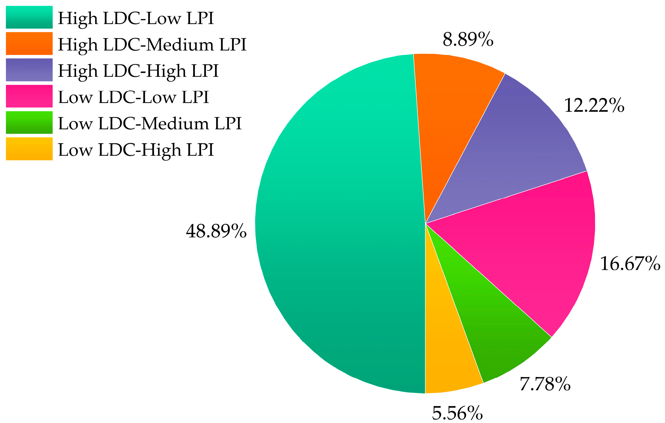
And then, this sample set is divided into two parts, a training set of 90 samples and a test set of 20 samples. In the training set, the distribution of samples on different gas well types is shown in Figure 3.

It can be seen that the samples in the training set are obviously unevenly distributed, and this should be paid special attention during the analysis process.

2.2. Procedures and Methods

Simple and intuitive classification maps bring great convenience to the field application, and are also the key to realize the rapid evaluation and diagnosis of gas wells. Considering the large amount of available production data and industrial knowledge accumulated on site, this paper aims to establish gas well classification maps through the analysis and mining of production data, and enables a production data-driven gas well classification. During this process, the dimensionality reduction technique is used to fuse the features to construct the visualized classification space, namely, the decision space for gas well classification, and then the classification algorithm is employed to determine the classification boundaries in the decision space.

Specifically, in this paper, four dimensionality reduction techniques, LDA, PCA, LPP and ICA, are introduced to process the sample data before classification training, such that different visualized low-dimensional spaces are constructed, and at the same time, the original samples are projected into these low-dimensional spaces, forming several sets of low-dimensional samples. Then, four classical classification algorithms, NB, DA, KNN, and SVM, are individually trained and evaluated on each set of samples, so as to quantify the performance of the algorithms in the each low-dimensional space. Based on the performance of the algorithms, efforts are made to find the most effective dimensionality reduction technique and its best-matched classification algorithm. Therefore, this paper is devoted to specifying the most excellent combination of the dimensionality reduction technique and the classification algorithm, that is, to proposing the optimal data processing flow for the establishment of gas well classification maps.

As a result, a combination model composed of the dimensionality reduction technique and the classification algorithm will be developed. With this model, the gas well classification map can be established based on production data, achieving production data-driven gas well classification. Once a classification map is established, new gas well samples can be projected onto the map to perform a rapid evaluation and diagnosis, thereby providing timely decision-making support for their routine management.

2.2.1. Dimensionality Reduction Techniques

In this paper, linear dimensionality reduction techniques are chosen to reduce the dimensionality of the original sample data from the training set. This is based on the fact that for linear dimensionality reduction techniques, samples are projected from a high-dimensionality space to a low-dimensionality space by a linear transformation. This means that each feature of the low-dimensionality data is a linear combination of the features of the high-dimensionality data. Moreover, the projection vectors, which specify this combination manner, can be explicitly provided during the dimensionality reduction process. Consequently, after establishing the gas well classification map, new samples (out-of-sample data) can be readily and promptly projected onto the map using the obtained projection vectors, enabling fast classification and diagnosis. Therefore, in order to facilitate the dimensionality reduction of new sample data and to apply the classification results to the evaluation of new samples, four common linear dimensionality reduction techniques are chosen to process the original sample data: PCA, LDA, ICA, and LPP. These techniques aim to capture the most significant information of the original sample data from their unique perspectives.

(1)

Principal Component Analysis (PCA)

Principal Component Analysis (PCA) is one of the most famous unsupervised dimensionality reduction techniques. The goal of the PCA technique is to find the PCA space to transform the data from a higher-dimensional space to a lower-dimensional space. The PCA space consists of k principal components and those principal components are orthonormal, uncorrelated, and each principal component represents the direction of the maximum variance. The first principal component (PC1) of the PCA space represents the direction of the maximum variance of the data, the second principal component has the second largest variance, and so on [18]. The PCA technique projects the data into a lower-dimensional subspace where the sample variance is maximized.

(2)

Linear Discriminant Analysis (LDA)

Linear Discriminant Analysis (LDA), or Fisher Discriminant Analysis, is also a well-known technique for feature extraction and dimension reduction. It has been used widely in many applications such as face recognition, image retrieval, microarray data classification, etc. [19]. Compared with PCA, LDA is a supervised learning technique. LDA takes a set of high-dimensional data, which is grouped into classes, as its input to find an optimal transformation (projection) that maps the raw data into a lower-dimensional space while preserving the class structure. This transformation (projection) minimizes the within-class distance and simultaneously maximizes the between-class distance, thus achieving maximum discrimination [20]. In other words, if the multiclass raw data are mean-based, its different classes will achieve excellent separation in the LDA low-dimensional space.

(3)

Locality Preserving Projection (LPP)

Locality Preserving Projection (LPP) is a linear projective map that arises by solving a variational problem that optimally preserves the neighborhood structure of the dataset [21]. This technique is essentially a linear extension of Laplacian eigenmaps and aims to seek optimal projections while preserving the local geometry in original data. It constructs the proximity relationship between samples in the space, and preserves such proximity relationship as much as possible in the dimensionality reduction projection, thus preserving the local structure of the data [22]. Compared with PCA, etc., when the dataset has a nonlinear manifold structure, the local retained projection shows better projection performance.

(4)

Independent Component Analysis (ICA)

ICA belongs to the blind source separation (BSS) method that is used to separate data into underlying informational components. The term “blind” is intended to imply that such methods can separate data into source signals even if very little is known about the nature of those source signals. ICA is based on the simple, generic, and physically realistic assumption that if different signals are from different physical processes (e.g., different people speaking), then those signals are statistically independent. Accordingly, ICA separates signal mixtures into statistically independent signals. If the assumption of statistical independence is valid, then each of the signals extracted by independent component analysis will have been generated by a different physical process, and will therefore be a desired signal [23].

In the aforementioned algorithms, PCA and ICA are implemented using the built-in functions provided by the Statistics and Machine Learning Toolbox in Matlab (R2023a Update 2: 9.14.0.2254940), while LDA and LPP are implemented by programming on the Matlab platform.

2.2.2. Classification Algorithms

After the dimensionality reduction, the classification algorithm is trained on the samples projected into the low-dimensional space, allowing it to build a comprehension of the low-dimensional samples and obtain the ability to distinguish the types of gas wells in the specified low-dimensional space. In order to sift out the most effective dimensionality reduction technique among the four aforementioned techniques and, subsequently, match the best classification algorithm for it, several classical classification algorithms are, respectively, trained and evaluated on the low-dimensional samples generated by each of the four dimensionality reduction techniques. The performance of these algorithms in each low-dimensional space is taken as the criterion to find the optimal dimensionality reduction technique and its best-matched classification algorithm. In this paper, four classical classification algorithms, NB, DA, KNN, and SVM, are selected to be trained on the sample data after dimensionality reduction.

(1)

Naive Bayes (NB)

Naive Bayes is one of the most efficient and effective inductive learning algorithms for machine learning and data mining [24]. It is based on simplifying Bayes theorem by the naive assumption that the features are independent of each other [12]. And it provides a mechanism for using the information in sample data to estimate the posterior probability P(y|x) of each class y given an object x. Once such estimates are obtained, they can be used for classification or other decision support applications [25].

(2)

Discriminant Analysis (DA)

Discriminant analysis is a multivariate statistical analysis method to determine the type of a research object according to its various feature values under the condition that the classification is determined. Its basic principle is to establish one or more discriminant functions according to certain discriminant criteria, to determine the undetermined coefficients in the discriminant functions with a large amount of data of the research object. When obtaining a new sample, calculating the discriminant indexes, the classification of the sample can be determined [26]. According to the form of discriminant function, it can be divided into linear discriminant analysis and nonlinear discriminant analysis; According to different discriminant criteria, it can be divided into distance discriminant analysis, Fisher discriminant analysis, Bayes discriminant analysis, and so on [27]. When Fisher’s criterion is used as the discriminant analysis criteria, that is, the projection method is adopted, discriminant analysis can be used for dimensionality reduction, as described in the previous section.

(3)

K-Nearest Neighbor (KNN)

K-nearest neighbor is a very powerful tool; it combines classification and regression algorithms based on distance calculation between instances [28]. The KNN is a non-parametric method classifying an object by a majority vote of its neighbors [29]. This method treats samples as points in n-dimensional feature space. To classify a sample from the test set, it looks up the k samples from the training set with the shortest Euclidean distance to the test sample and picks the most common class among them [12]. The choice of K value greatly affects the algorithm performance. In this paper, the number of nearest k points is evaluated by using K-fold validation.

(4)

Support Vector Machine (SVM)

Like k-nearest neighbor classifiers, SVMs treat samples as points in feature space. SVMs, however, work by constructing hypersurfaces that optimally separate different classes’ sample clusters [12]. The guiding rule is based on maximizing the margin between the hyperplane and the observations. This method relies more on the data points closest to the decision boundary, and as a result is less influenced by outlier data points [30].

All four classification algorithms are implemented using built-in functions from the Statistics and Machine Learning Toolbox in Matlab, and parameters not mentioned are set to default values defined by the toolbox.

2.2.3. Model Training and Evaluation

As the sample size of the current task is small, the approach of k-fold cross-validation is used to train the classification algorithm and evaluate its performance. In k-fold cross-validation, the original sample is randomly partitioned into k equal-sized subsamples. Of the k subsamples, a single subsample is retained as the validation data for testing the model, and the remaining k − 1 subsamples are used as training data. The cross-validation process is then repeated k times, with each of the k subsamples used exactly once as the validation data. Finally, k different accuracy or other evaluation indicators are obtained, and the average value of these indicators is calculated to estimate the performance of the algorithm [31]. The superiority of this approach is that all observations are used for both training and validation, thereby effectively avoiding issues arising from unreasonable data partitioning, such as overfitting. This is particularly beneficial when dealing with small-scale datasets. Taking into account the size of the training sample set, this paper adopts 5-fold cross-validation.

Standard evaluation indicators from machine learning are employed to evaluate the performance of classification algorithms. These indicators typically include Accuracy, Precision, Recall, and F1-score. The confusion matrix is the standard format for algorithm performance evaluation, and it is also the basis for the calculation of the above evaluation indicators. Binary classification is taken as an example to illustrate these indicators. This classification task considers two classes in general: the positive example class and the negative example class, and its confusion matrix consists of four important parameters that are used to count the classification results: TP, TN, FP, and FN. For these four parameters, the first letter indicates whether the predicted result matches the real result, that is, whether the predicted result is correct, with correct: T, incorrect: F. The second letter represents the response of the algorithm to the sample, that is, it describes the output result of the algorithm to the sample, with positive example: P, negative example: N. Therefore, the meanings of the four parameters are as follows: TP, the number of samples which are correctly predicted as the positive sample; TN, the number of samples which are correctly predicted as the negative sample; FP, the number of samples which are incorrectly predicted as the positive example; FN, the number of samples which are incorrectly predicted as the negative example. On this basis, the above evaluation indicators are defined as follows.

Accuracy: the proportion of samples that are correctly predicted in total samples.

Accuracy = (TP + TN)/(TP + FP + TN + FN),

(1)

Precision: the proportion of positive samples that are correctly predicted to be positive in all samples that are predicted to be positive. This indicator also indicates the possibility of misreporting.

Precision = TP/(TP + FP),

(2)

Recall: the proportion of positive samples that are correctly predicted to be positive in all samples that are truly positive. This indicator also indicates the possibility of underreporting.

Recall = TP/(TP + FN),

(3)

F1-score: the harmonic mean of precision and recall. This indicator is a good balance between precision and recall, especially when there is an uneven class distribution.

F1-score = 2 × (Precision × Recall)/(Precision + Recall),

(4)

For the multi-class classification task, it is usually divided into several binary classification tasks, and its evaluation indicators are calculated based on each extended binary classification confusion matrix. The extended binary confusion matrix is constructed according to the following steps. In the investigation of a certain class, the current class is regarded as the positive example class, and the remaining classes are regarded as the negative example class. Doing this across all classes, the values of TP, FP, TN, FN for each class can be obtained.

At this point, there are two common methods to obtain the evaluation indicators of the whole classification task; they are Macro-average and Micro-average. The Macro-average method firstly calculates the evaluation indicators (Precision, Recall, and F1-score) for each class in isolation, and then averages the evaluation indicators over all classes to obtain the Macro evaluation indicators (Macro Precision, Macro Recall, and Macro F1-score). The Micro-average method firstly sums the predicted results of samples (i.e., TP, FP, and FN) across all classes, then calculates the global Precision, Recall, and consequently F1-score, according to the definition. Namely, the Micro Precision, Micro Recall, and Micro F1-score [32,33]. It can be seen that Macro-average considers equally important the effectiveness in each class, independently of the relative size of the class, and can fully consider the performance of classifier on the small sample class. In contrast, Micro-average considers equally important the effectiveness of each sample, independently of its class, and measures the capability of the algorithm to correctly predict the class on a per-sample basis. Thus, the two types of metrics provide complementary assessments of the classification effectiveness [34]. It is worth noting that as the Macro-average pays enough attention to the performance of the algorithm on smaller classes, Macro-average indicators are especially important when the class distribution is uneven and skewed, such as in the case of that there is a wide variation in the number of samples among different gas well types.

3. Results and Discussion

3.1. New Feature Spaces and 2D Samples

Before dimensionality reduction, Min-Max normalization is performed on the original sample data, and in PCA dimensionality reduction, the original sample data are further centered. The dimensionality of the target space is specified as two; thus, PCA retains the first two principal components to construct the new feature space, and for LDA, it retains the first two projection directions to construct the LDA space. In LPP and ICA, the number of features to be extracted is set to two. In addition, by trial validation, it is recommended to conduct LPP based on six neighbors to achieve the optimal effect.

Through dimensionality reduction, the five original features are fused into four pairs of new features under different extraction principles, thus constructing four new feature spaces. Simultaneously, linear transformations that fuse the original features into these new salient features are obtained. The projection vectors corresponding to these linear transformations are presented in

Table 2. Projection vectors of different dimensionality reduction (DR) techniques.

DR Technique	Projection Vector	Vector Value
PCA	Vector 1	(−0.0726	0.4697	0.5183	0.6021	0.3781)T
	Vector 2	(−0.0579	−0.4028	−0.5381	0.3690	0.6392)T
LDA	Vector 1	(−0.0827	0.1917	−0.0616	0.9299	0.2965)T
	Vector 2	(0.2540	0.9157	0.2033	−0.2089	−0.1092)T
LPP	Vector 1	(−0.0222	−0.0405	−0.0242	−0.0047	−0.0048)T
	Vector 2	(−0.0352	−0.0269	−0.0206	0.0926	0.1022)T
ICA	Vector 1	(0.2955	−0.3957	−0.5513	−0.6128	−0.2769)T
	Vector 2	(−0.8122	−0.4856	0.0624	0.3164	0.0213)T

.

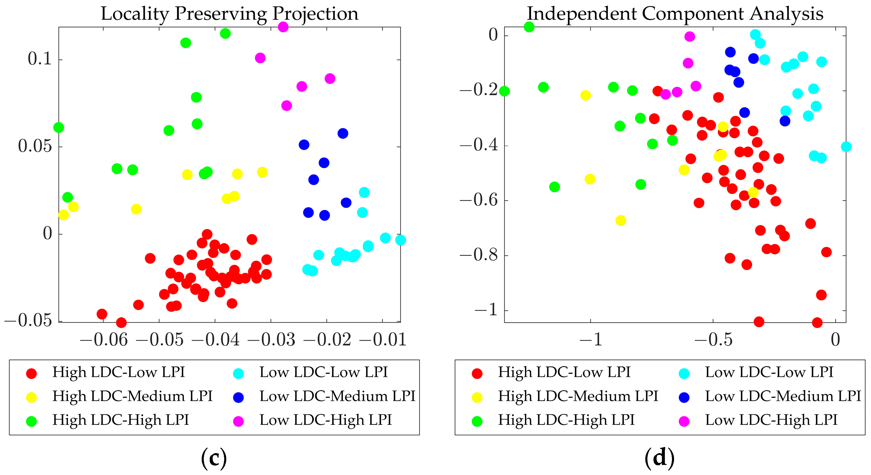
On the other hand, during this process, the original samples are projected into distinct two-dimensionality (2D) feature spaces, resulting in four sets of two-dimensionality (2D) samples. For each set of 2D samples, their distribution in the respective 2D feature space is displayed in Figure 4.

The sample distribution intuitively demonstrates that the samples exhibit the most distinct separation in the LDA space, followed by the LPP space. In the PCA space, while the samples are well separated on the whole, there are a few instances of poor separation locally. The ICA space yields the least effective separation of samples.

Building upon this foundation, to quantitatively identify the optimal sample separation space among the four 2D spaces, referred to as the decision space for gas well classification, and to match the best classification algorithm to determine the classification boundary in this decision space, various classification algorithms are trained on these four sets of 2D samples. Based on the performance of the classification algorithms on each set of 2D samples, the ideal combination of dimensionality reduction method and classification algorithm can be specified for the gas well classification task, thereby proposing the optimal data processing flow for establishing gas well classification maps.

3.2. Classification Map Establishment

During the classification training process, NB assumes that for each feature variable of the sample, its conditional probability follows a Gaussian distribution, and a separate Gaussian distribution is estimated for each class. DA is performed based on the Fisher discriminant criteria, and with the assumption that all classes have the same covariance matrix. In KNN, the hyper parameter k (number of nearest neighbors) is optimized by implementing five-fold cross-validation on the training samples, and the value of k is specified as 5. In SVM, a Gaussian function is employed as the kernel function, and the multiclass classification is achieved by combining multiple binary classifications. For each binary classification, one class is taken as positive, another as negative, and the rest of the classes are ignored, i.e., the so-called one-versus-one approach is adapted. Furthermore, for all four classification algorithms, the prior probabilities for each class are considered to be the same.

3.2.1. Construction of Decision Space

Based on five-fold cross-validation, the four classification algorithms are trained on each set of 2D samples, and the performance of these algorithms in each 2D space is evaluated. In addition, in order to further eliminate the impact of data partitioning on the training results, the 5-fold cross-validation is repeated four times. As an illustration, for one of these 5-fold cross-validations, the performance evaluation indicators of the classification algorithms in each 2D space are listed in

Table 3. Performance evaluation indicators of the classification algorithms in the PCA space.

Combination Case	Accuracy (%)	Macro			Micro
		Precision (%)	Recall (%)	F1-score (%)	Precision (%)	Recall (%)	F1-score (%)
PCA-NB	92.963	67.649	72.341	69.321	78.889	78.889	78.889
PCA-DA	92.963	69.275	73.862	69.473	78.889	78.889	78.889
PCA-KNN	93.704	69.861	77.594	71.153	81.111	81.111	81.111
PCA-SVM	94.074	73.591	78.270	72.547	82.222	82.222	82.222

,

Table 4. Performance evaluation indicators of the classification algorithms in the LDA space.

Combination Case	Accuracy (%)	Macro			Micro
		Precision (%)	Recall (%)	F1-score (%)	Precision (%)	Recall (%)	F1-score (%)
LDA-NB	98.148	92.158	92.715	92.066	94.444	94.444	94.444
LDA-DA	99.259	96.875	97.538	97.049	97.778	97.778	97.778
LDA-KNN	98.889	93.472	94.886	94.021	96.667	96.667	96.667
LDA-SVM	98.889	93.056	94.886	93.624	96.667	96.667	96.667

,

Table 5. Performance evaluation indicators of the classification algorithms in the LPP space.

Combination Case	Accuracy (%)	Macro			Micro
		Precision (%)	Recall (%)	F1-score (%)	Precision (%)	Recall (%)	F1-score (%)
LPP-NB	98.148	90.593	92.828	90.464	94.444	94.444	94.444
LPP-DA	97.037	84.306	86.281	84.752	91.111	91.111	91.111
LPP-KNN	95.556	76.369	79.758	76.705	86.667	86.667	86.667
LPP-SVM	90.370	56.878	61.885	55.359	71.111	71.111	71.111

and

Table 6. Performance evaluation indicators of the classification algorithms in the ICA space.

Combination Case	Accuracy (%)	Macro			Micro
		Precision (%)	Recall (%)	F1-score (%)	Precision (%)	Recall (%)	F1-score (%)
ICA-NB	90.370	64.395	66.407	64.264	0.71111	71.111	71.111
ICA-DA	89.630	61.236	67.361	62.146	0.68889	68.889	68.889
ICA-KNN	87.037	60.265	65.933	60.624	0.61111	61.111	61.111
ICA-SVM	90.741	61.215	67.985	60.806	0.72222	72.222	72.222

. The corresponding confusion matrices are shown in Appendix B.

As observed from the above tables, the evaluation results of the Accuracy and Micro indicators are consistent, but at times, the Macro indicators give different opinions. This divergence stems from the fact that the Accuracy and Micro indicators do not account for the influence of classes and solely focus on the sample itself, while the Macro indicators consider the classification effect of each class. Moreover, it is apparent that in some instances, the Accuracy and Micro indicators cannot effectively distinguish the performance of different algorithms. Therefore, in the current scenario of uneven sample distribution across different classes, the Macro indicators are employed to evaluate the algorithm performance. Furthermore, the comprehensive indicator F1-score, which combines Precision and Recall, is selected as the criterion. Additionally, it is also noteworthy that all Micro indicators have the same value, which is inherent to their definition.

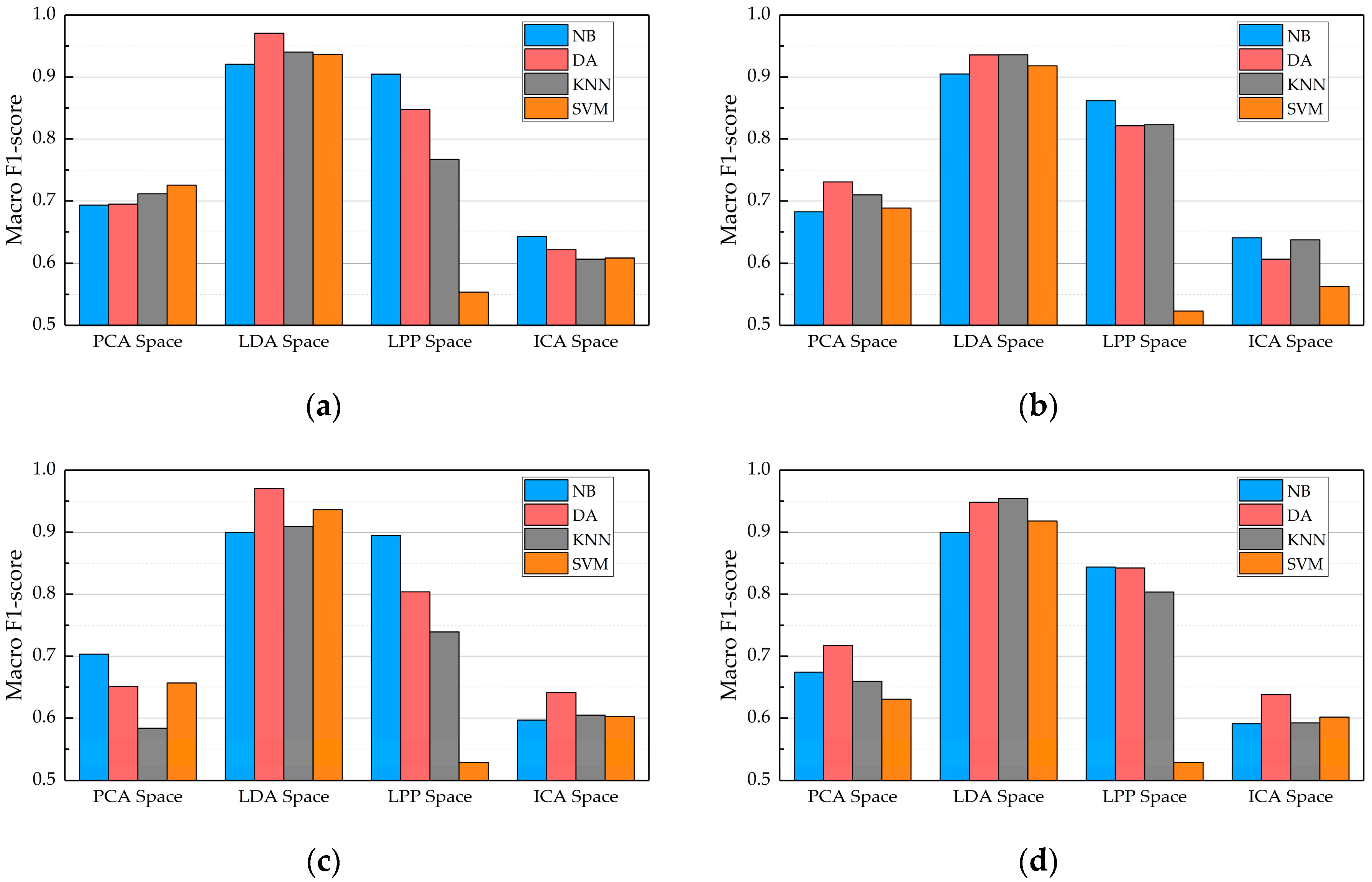
The Macro F1-scores of the four algorithms in different 2D spaces are compared, and the comparison results of four five-fold cross-validations are depicted in Figure 5.

The results from the four five-fold cross-validations illustrate that even when the sample set is randomly divided in each cross-validation, the training and evaluation of the algorithms are still influenced by the sample partitioning. Despite this, synthesizing the results from the four cross-validations, it can be also concluded that that, in line with the intuitive understanding of dimensionality reduction effects, the classification algorithms all achieve high scores in the LDA space. Secondly, in the LPP space, apart from SVM, the other three algorithms also obtain relatively high scores. However, the performance of the four algorithms in the PCA space is unsatisfactory, and almost no algorithm achieves effective classification in the ICA space.

Hence, from a quantitative perspective, training results once again demonstrate that the LDA technique achieves optimal separation of different types of gas well samples and offers the optimal space for operating the classification algorithms. As a result, the LDA technique is employed to construct the decision space for gas well classification. The superior performance of LDA may be attributed to its nature as a supervised dimensionality reduction method, allowing it to leverage more sample information during the dimensionality reduction process. Furthermore, it can be seen that there are substantial discrepancies in classification algorithm performance across different spaces; this indicates that the construction of the decision space plays a crucial role in achieving successful gas well classification.

3.2.2. Determination of Classification Boundary

In order to designate the best-matched classification algorithm for the chosen dimensionality reduction technique, and consequently determine the classification boundaries in the decision space, the average of the Macro F1-scores from the four cross-validations is utilized as the final criterion to evaluate the performance of the four classification algorithms. For different 2D spaces, the Average Macro F1-score of each classification algorithm across the four cross-validations is shown in Figure 6.

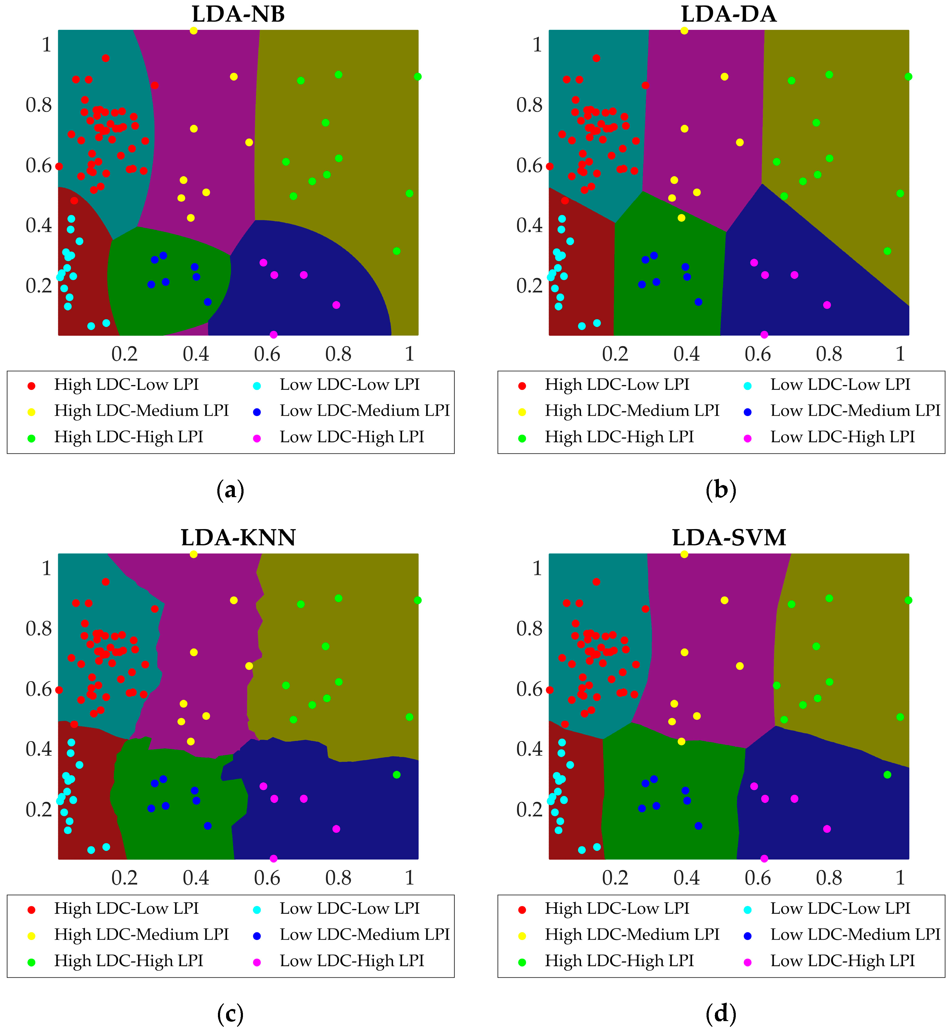
In the chosen LDA decision space, the four classification algorithms achieve Average Macro F1-scores of 90.606% (NB), 95.619% (DA), 93.502% (KNN), and 92.712% (SVM), respectively. It can be seen that the LDA algorithm achieves the highest score, followed closely by the KNN and SVM algorithms, while the NB algorithm’s score is comparatively less prominent. However, it is important to note that although the KNN and SVM algorithms obtain decent scores in the LDA space, their performance in the LPP space (where the sample separation is suboptimal but also effective) is disappointing, especially for the SVM algorithm. In the LPP space, the Average Macro F1 score for the KNN algorithm is 78.323%, while the SVM algorithm’s score is as low as 53.361%. This is because of the fact that for the current gas well classification task, both k-nearest neighbor (KNN) and support vector machine (SVM) algorithms exhibit excessive complexity; when the dataset contains redundancy and noise, they are more likely to generate complex decision boundaries (this can be confirmed in subsequent chapters), leading to overfitting and thus significantly degrading their own performance. Given these findings, there are sufficient reasons to employ the DA algorithm to determine the classification boundaries for different gas well types.

Additionally, it is also worth noting that, as shown in Figure 5, in the current LDA decision space, the DA algorithm consistently achieves convincing scores (maximum or slightly lower) across all four cross-validations (which correspond to different training samples), indicating its excellent robustness for the current classification task. This further bolsters the proposition of utilizing the DA algorithm to determine the classification boundaries in the decision space. On the other hand, it also illustrates that the algorithm with appropriate complexity can maintain considerable performance across a wide range of data, which is an important guarantee for achieving accurate and effective gas well classification.

3.2.3. Combination Model and Classification Maps

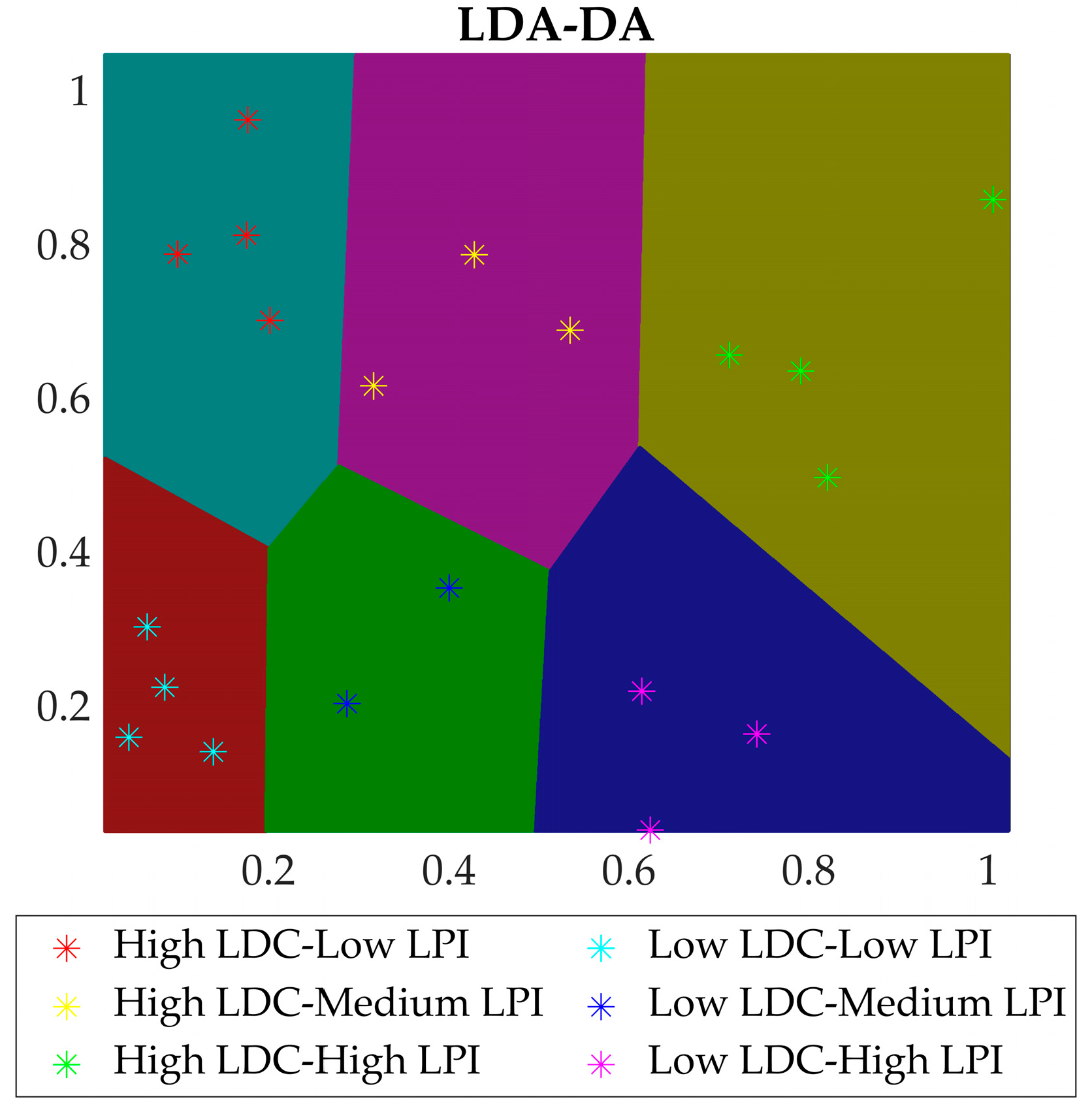
Up to this point, the optimal combination of dimensionality reduction techniques and classification algorithms has been specified, and accordingly, the optimal data processing flow for establishing the gas well classification map has been defined. To be specific, this flow can be outlined as follows. After feature engineering, the LDA technique is initially used to fuse the five features, constructing the 2D decision space for gas well classification, and simultaneously projecting the original samples into this 2D LDA space to form the training samples. Then, the DA algorithm is trained on all the 2D samples so as to build classification rules, and in turn, determine the classification boundaries in the LDA decision space, ultimately forming the gas well classification map.

It is evident that this process has proposed a model capable of establishing a gas well classification map through the analysis and mining of sample data. Moreover, this model combines the Linear Discriminant Analysis dimensionality reduction technique and the Discriminant Analysis classification algorithm, and as such, it is referred to as the LDA-DA (Linear Discriminant Analysis–Discriminant Analysis) combination model. Using the LDA-DA combination model, a gas well classification map is established based on the current sample data, as depicted in Figure 7. To illustrate the classification effects of different algorithms, Figure 7 also presents the maps drawn by the other three classification algorithms in the LDA space.

It can be seen that in the LDA decision space, different classification algorithms yield different classification boundaries. Compared to the other three algorithms, the DA algorithm provides linear classification boundaries, which are more concise and suitable for on-site applications. However, it is worth noting that, according to the previous analysis, among the four classification algorithms, the performance of the DA algorithm is still the best. This indicates that an algorithm with appropriate complexity can contribute concise classification boundaries while ensuring accurate and effective gas well classification.

3.3. Test and Verification

With the reserved test set samples, the experiment is conducted to test the classification effect of the classification map, and thus verify its validity and practicability. The samples in the test set are listed in

Table 7. Samples in the test set.

No.	SP	C-GFR	SRGP	C-LFR	LGR-SD	Type Label
	MPa	104 m3/d	104 m	m3/d	Fraction
Sample 1	16.27	6.0183	63.8500	0.91	0.0453	High LDC-Low LPI
Sample 2	8.05	5.7952	274.0215	3.39	0.3287	High LDC-Low LPI
Sample 3	9.57	7.0454	514.0142	2.95	0.0814	High LDC-Low LPI
Sample 4	9.89	6.2014	390.2455	2.94	0.2305	High LDC-Low LPI
Sample 5	11.04	6.5031	352.4357	7.75	1.2896	High LDC-Medium LPI
Sample 6	8.62	6.2695	244.0125	12.69	0.6965	High LDC-Medium LPI
Sample 7	15.05	4.9272	345.2147	5.04	1.5985	High LDC-Medium LPI
Sample 8	3.32	7.1369	85.0572	11.82	3.1957	High LDC-High LPI
Sample 9	10.24	7.8594	397.2941	25.92	1.1026	High LDC-High LPI
Sample 10	10.62	6.2054	277.0124	16.64	1.4294	High LDC-High LPI
Sample 11	3.48	5.7215	260.1546	21.24	0.9811	High LDC-High LPI
Sample 12	2.86	2.3218	178.4257	3.26	0.5158	Low LDC-Low LPI
Sample 13	3.76	3.2245	186.2547	1.34	0.1085	Low LDC-Low LPI
Sample 14	2.60	3.1015	5.5473	0.87	0.3154	Low LDC-Low LPI
Sample 15	2.20	2.5864	12.3851	0.64	0.1120	Low LDC-Low LPI
Sample 16	5.36	3.1536	8.5190	5.41	1.0790	Low LDC-Medium LPI
Sample 17	1.20	4.5100	74.7258	8.45	0.7977	Low LDC-Medium LPI
Sample 18	2.15	3.9524	76.9765	12.59	1.9625	Low LDC-High LPI
Sample 19	2.38	2.2037	341.9542	17.28	1.2984	Low LDC-High LPI
Sample 20	5.21	3.7225	18.9524	15.21	2.6050	Low LDC-High LPI

.

Taking the projection vector pair of the LDA space, (−0.0827, 0.1917, −0.0616, 0.9299, 0.2965)^T and (0.2540, 0.9157, 0.2033, −0.2089, −0.1092)^T, twenty test samples are projected onto the LDA-DA gas well classification map, as shown in Figure 8. Note that, prior to the projection, the test samples are preprocessed using the same normalization mapping as the samples in the training set.

The distribution of the test samples shows that the classification map successfully distinguishes between different types of gas wells, and the classification results are quite consistent with the field experts. This indicates that the LDA-DA classification map is reasonable and reliable, and also demonstrates the effectiveness of the LDA-DA model for the current classification task. Furthermore, it can also be concluded from the above process that once the classification map is established, a rapid and intuitive evaluation and diagnosis of gas well production status can be realized only through simple processing of production data. On this basis, when combined with the chart of recommended treatment measures in Figure 2, timely decision-making support can be provided for the routine management of gas wells, thus guiding the formulation of management strategies and the implementation of liquid loading treatment measures.

4. Conclusions

(1)

A production data-driven method for gas well classification is proposed, which classifies gas wells from the perspective of instant evaluation and short-term management strategy decision making, and establishes classification rules through the analysis and mining of production data. This offers new ideas on gas well classification, expanding its content and scope, and thus holds certain guiding significance for research in this field.

(2)

Feature engineering is the foundation of gas well classification. This paper applies domain knowledge to feature engineering, successfully interpreting and processing the gas well production data according to the current usage scenario, ensuring the pertinence and purposiveness of feature extraction. In similar classification tasks, if unavoidable considerations from other aspects arise, it is necessary to re-implement feature engineering.

(3)

The classification map can be continuously updated in field applications. It means that new samples are constantly added, inapplicable samples are removed, and the upgraded sample set is used to regenerate the map. This allows the classification map to continuously acquire new knowledge to adapt to the gas reservoir development process. Additionally, if an automatic data collection system is deployed in the field and the data processing flow described in this paper is integrated into program modules, the current work has the potential to evolve into an online, self-updating gas well classification and diagnostic system, providing real-time decision-making support for the routine management of gas wells.

References

1. Liu, J.; Zhu, Z.; Hong, J.; Feng, X.; Yang, Y.; Guo, J.; Wang, D. Gas well classification method based on production data characteristic analysis. Oil Drill. Prod. Technol. 2021, 43, 510–517. [Google Scholar] [CrossRef]
2. Liu, C. Analysis of Production Characteristics and Technical Countermeasures of Gas Wells in Shenmu Gas Field. Master’s Thesis, Xi’an Shiyou University, Xi’an, China, 2018. [Google Scholar]
3. Joseph, A.; Sand, C.M.; Ajienka, J.A. Classification and Management of Liquid Loading in Gas Wells. In Proceedings of the SPE Nigeria Annual International Conference and Exhibition, Lagos, Nigeria, 5–7 August 2013. [Google Scholar]
4. Wei, Y.; Jia, A.; He, D.; Liu, Y.; Ji, G.; Cui, B.; Ren, L. Classification and evaluation of horizontal well performance in Sulige tight gas reservoirs, Ordos Basin. Nat. Gas Ind. 2013, 33, 47–51. [Google Scholar]
5. Zhang, N. Classification evaluation of production dynamic for horizontal well in Su 53 block. Unconv. Oil Gas 2021, 8, 88–94. [Google Scholar] [CrossRef]
6. Qiu, L. Dynamic Analysis of Tight Water-Producing Gas Reservoirs and Evaluation of Water Production Impact in Western Sulige Area. Master’s Thesis, Xi’an Shiyou University, Xi’an, China, 2020. [Google Scholar]
7. Shang, Y.; Zhai, S.; Lin, X.; Li, X.; Li, H.; Feng, Q. Dynamic and static integrated classification model for low permeability tight gas wells based on XGBoost algorithm. Spec. Oil Gas Reserv. 2023, 30, 135–143. [Google Scholar]
8. Zhang, Z. Well Management and Dynamic Analysis of Eastern Sulige Gasfield. Master’s Thesis, Xi’an Shiyou University, Xi’an, China, 2016. [Google Scholar]
9. Sharma, A.; Srinivasan, S.; Lake, L.W. Classification of Oil and Gas Reservoirs Based on Recovery Factor: A Data-Mining Approach. In Proceedings of the SPE Annual Technical Conference and Exhibition, Florence, Italy, 19–22 September 2010. [Google Scholar]
10. Lee, B.B.; Lake, L.W. Using Data Analytics to Analyze Reservoir Databases. In Proceedings of the SPE Annual Technical Conference and Exhibition, Houston, TX, USA, 28–30 September 2015. [Google Scholar]
11. Barone, A.; Sen, M.K. An Improved Classification Method That Combines Feature Selection with Nonlinear Bayesian Classification and Regression: A Case Study on Pore-Fluid Prediction. In Proceedings of the 2017 SEG International Exposition and Annual Meeting, Houston, TX, USA, 24–29 September 2017. [Google Scholar]
12. Viggen, E.M.; Løvstakken, L.; Ma, S.-E.; Merciu, I.A. Better automatic interpretation of cement evaluation logs through feature engineering. SPE J. 2021, 26, 2894–2913. [Google Scholar] [CrossRef]
13. Zhang, Y.; Hu, J.; Zhang, Q. Application of locality preserving projection-based unsupervised learning in predicting the oil production for low-permeability reservoirs. SPE J. 2021, 26, 1302–1313. [Google Scholar] [CrossRef]
14. Liao, L.; Zeng, Y.; Liang, Y.; Zhang, H. Data Mining: A Novel Strategy for Production Forecast in Tight Hydrocarbon Resource in Canada by Random Forest Analysis. In Proceedings of the International Petroleum Technology Conference, Dhahran, Saudi Arabia, 13–15 January 2020. [Google Scholar]
15. Ahmadi, R.; Aminshahidy, B.; Shahrabi, J. Data-driven analysis of stimulation treatments using association rule mining. SPE Prod. Oper. 2023, 38, 552–564. [Google Scholar] [CrossRef]
16. Ejim, C.; Xiao, J. Screening Artificial Lift and Other Techniques for Liquid Unloading in Unconventional Gas Wells. In Proceedings of the Abu Dhabi International Petroleum Exhibition and Conference, Abu Dhabi, United Arab Emirates, 9–12 November 2020. [Google Scholar]
17. Veeken, C.; Al Kharusi, D. Selecting Artificial Lift or Deliquification Measures for Deep Gas Wells in The Sultanate of Oman. In Proceedings of the SPE Kuwait Oil and Gas Show and Conference, Mishref, Kuwait, 13–16 October 2019. [Google Scholar]
18. Tharwat, A. Principal component analysis—A tutorial. Int. J. Appl. Pattern Recognit. 2016, 3, 197–240. [Google Scholar] [CrossRef]
19. Ye, J.; Janardan, R.; Li, Q. Two-Dimensional Linear Discriminant Analysis. In Proceedings of the Advances in Neural Information Processing Systems, Vancouver, BC, Canada, 13–18 December 2004. [Google Scholar]
20. Phinyomark, A.; Hu, H.; Phukpattaranont, P.; Limsakul, C. Application of linear discriminant analysis in dimensionality reduction for hand motion classification. Meas. Sci. Rev. 2012, 12, 82–89. [Google Scholar] [CrossRef]
21. Yu, W.; Teng, X.; Liu, C. Face recognition using discriminant locality preserving projections. Image Vision Comput. 2006, 24, 239–248. [Google Scholar] [CrossRef]
22. Zhang, L.; Qiao, L.; Chen, S. Graph-optimized locality preserving projections. Pattern Recogn. 2010, 43, 1993–2002. [Google Scholar] [CrossRef]
23. Stone, J.V. Independent Component Analysis: A Tutorial Introduction; The MIT Press: London, UK, 2004; pp. 5–11. [Google Scholar]
24. Zhang, H. The Optimality of Naive Bayes. In Proceedings of the Seventeenth International Florida Artificial Intelligence Research Society Conference, Miami Beach, FL, USA, 16–18 January 2004. [Google Scholar]
25. Webb, G.I. Naïve Bayes. In Encyclopedia of Machine Learning and Data Mining; Sammut, C., Webb, G.I., Eds.; Springer: Boston, MA, USA, 2016; pp. 1–2. [Google Scholar]
26. Brown, M.T.; Wicker, L.R. 8—Discriminant analysis. In Handbook of Applied Multivariate Statistics and Mathematical Modeling; Tinsley, H.E.A., Brown, S.D., Eds.; Academic Press: San Diego, CA, USA, 2000; pp. 209–235. [Google Scholar]
27. Mclachlan, G.J. General introduction. In Discriminant Analysis and Statistical Pattern Recognition; Mclachlan, G.J., Ed.; John Wiley & Sons, Ltd.: Hoboken, NJ, USA, 1992; pp. 1–26. [Google Scholar]
28. Alouhali, R.; Aljubran, M.; Gharbi, S.; Al-yami, A. Drilling Through Data: Automated Kick Detection Using Data Mining. In Proceedings of the SPE International Heavy Oil Conference and Exhibition, Kuwait City, Kuwait, 10–12 December 2018. [Google Scholar]
29. Bize-Forest, N.; Lima, L.; Baines, V.; Boyd, A.; Abbots, F.; Barnett, A. Using Machine-Learning for Depositional Facies Prediction in a Complex Carbonate Reservoir. In Proceedings of the SPWLA 59th Annual Logging Symposium, London, UK, 2–6 June 2018. [Google Scholar]
30. Biswas, D. Adapting Shallow and Deep Learning Algorithms to Examine Production Performance—Data Analytics and Forecasting. In Proceedings of the SPE/IATMI Asia Pacific Oil & Gas Conference and Exhibition, Bali, Indonesia, 29–31 October 2019. [Google Scholar]
31. Saini, I.; Singh, D.; Khosla, A. QRS detection using K-Nearest Neighbor algorithm (KNN) and evaluation on standard ECG databases. J. Adv. Res. 2013, 4, 331–344. [Google Scholar] [CrossRef] [PubMed]
32. Yang, Y. An evaluation of statistical approaches to text categorization. Inf. Retr. 1999, 1, 69–90. [Google Scholar] [CrossRef]
33. Durand, T.; Mehrasa, N.; Mori, G. Learning a Deep ConvNet for Multi-Label Classification With Partial Labels. In Proceedings of the 2019 IEEE/CVF Conference on Computer Vision and Pattern Recognition (CVPR), Long Beach, CA, USA, 15–20 June 2019. [Google Scholar]
34. Magno, G.; Rodrigues, T.; Almeida, V.A.F. Detecting Spammers on Twitter. In Proceedings of the Seventh annual Collaboration, Electronic messaging, AntiAbuse and Spam Conference, Redmond, WA, USA, 13–14 July 2010. [Google Scholar]
Figure 1. The site record from one gas well in the gas field.
Processes 12 01254 g001
Figure 2. The recommended treatment measures for different gas well types.
Processes 12 01254 g002
Figure 3. Distribution of samples on different gas well types.
Processes 12 01254 g003
Figure 4. Distribution of 2D samples in different 2D feature spaces: (a) PCA space; (b) LDA space; (c) LPP space; (d) ICA space.
Processes 12 01254 g004aProcesses 12 01254 g004b
Figure 5. Macro F1-scores of each algorithm in different 2D spaces: (a) Result 1 of the four 5-fold cross-verifications; (b) Result 2 of the four 5-fold cross-verifications; (c) Result 3 of the four 5-fold cross-verifications; (d) Result 4 of the four 5-fold cross-verifications.
Processes 12 01254 g005
Figure 6. Average Macro F1-scores of each algorithm in different 2D spaces.
Processes 12 01254 g006
Figure 7. Classification maps drawn by different classification algorithms: (a) LDA-NB classification map; (b) LDA-DA classification map; (c) LDA-KNN classification map; (d) LDA-SVM classification map. Note that, different background colors represent different regions of gas well types: indigo, high LDC-low LPI; pink, high LDC-medium LPI; tan, high LDC-high LPI; dark brown, low LDC-low LPI; dark green, low LDC-medium LPI; dark blue, low LDC-high LPI.
Processes 12 01254 g007
Figure 8. Distribution of the test samples in the LDA-DA classification map. Note that, different background colors represent different regions of gas well types: indigo, high LDC-low LPI; pink, high LDC-medium LPI; tan, high LDC-high LPI; dark brown, low LDC-low LPI; dark green, low LDC-medium LPI; dark blue, low LDC-high LPI.
Processes 12 01254 g008