

High-Density Polyethylene Pipe Butt-Fusion Joint Detection via Total Focusing Method and Spatiotemporal Singular Value Decomposition

Abstract
:1. Introduction
2. Principles of Algorithms
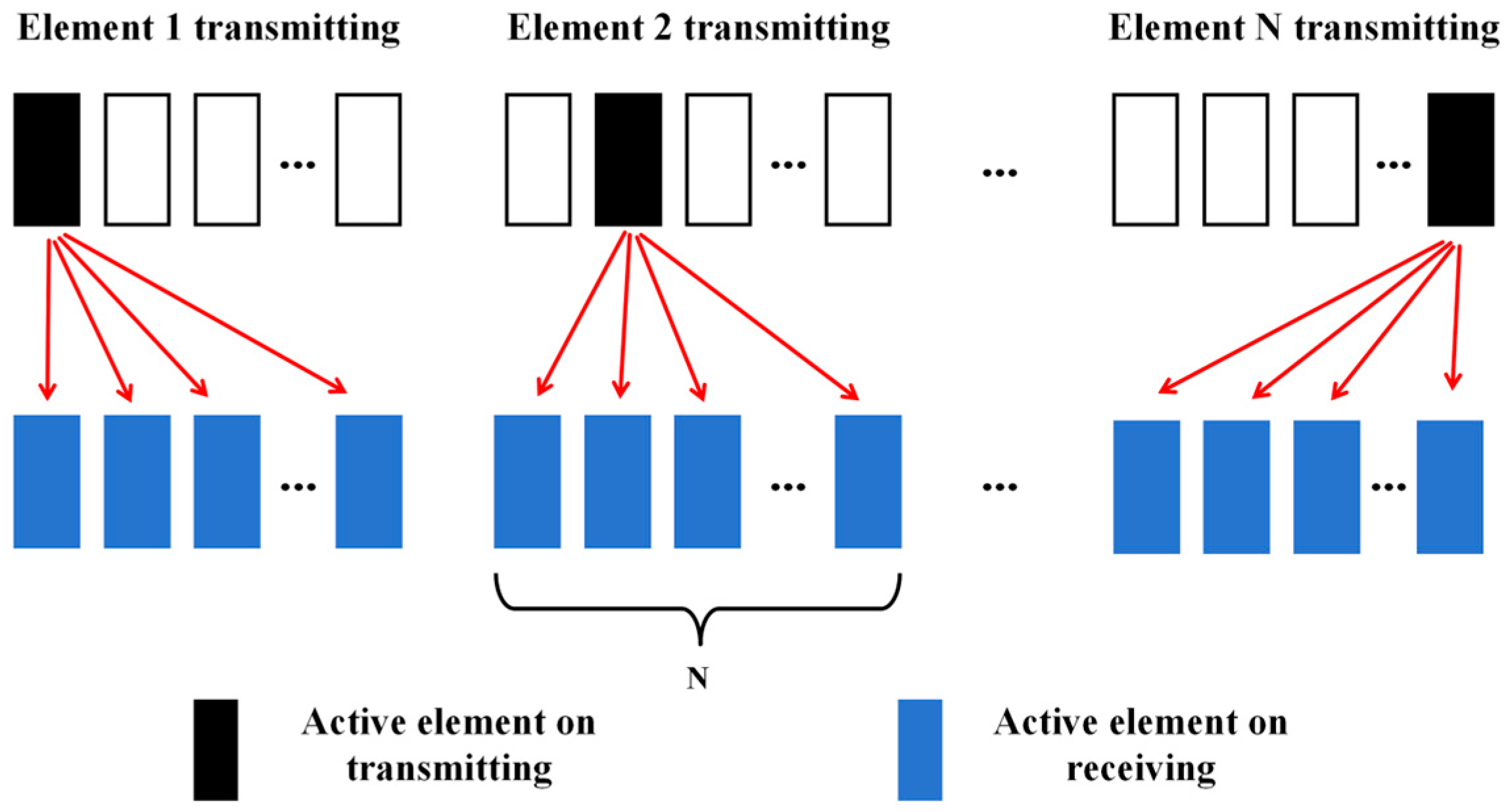
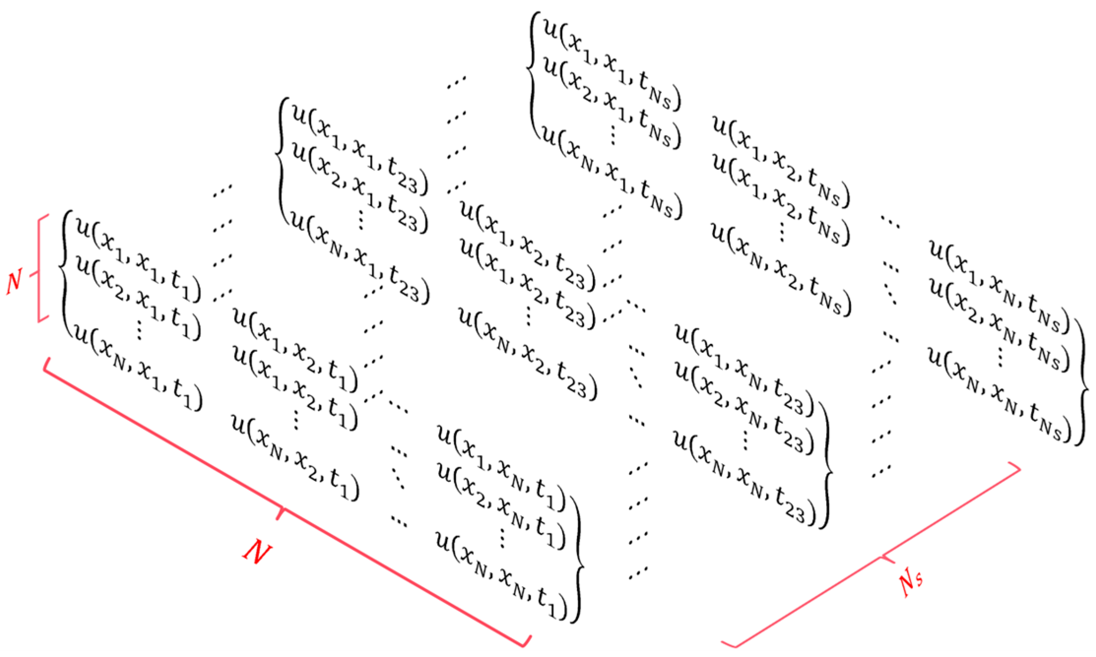
2.1. The Ultrasound Phased Array Data Based on FMC
2.2. STSVD Filtering Processing
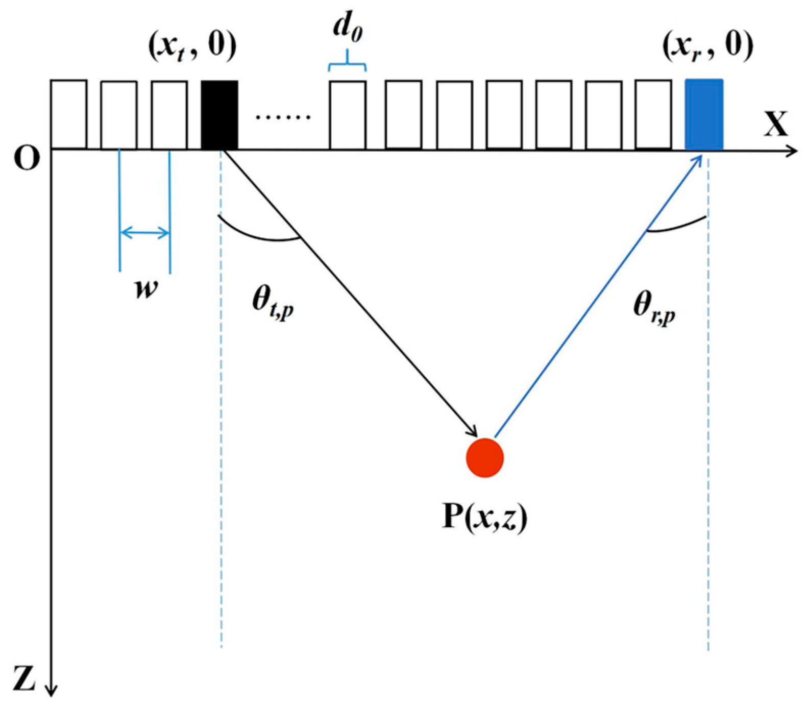
2.3. Improved Total Focusing Method
3. Experiments
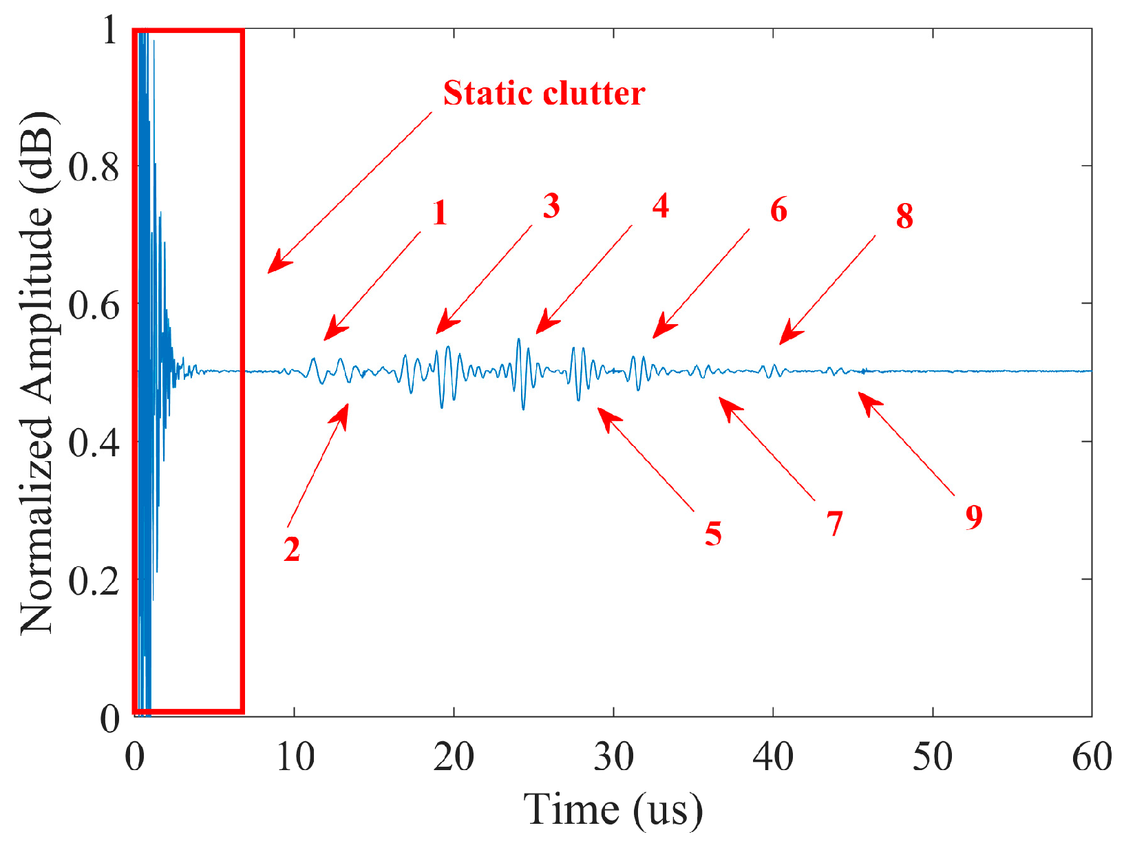
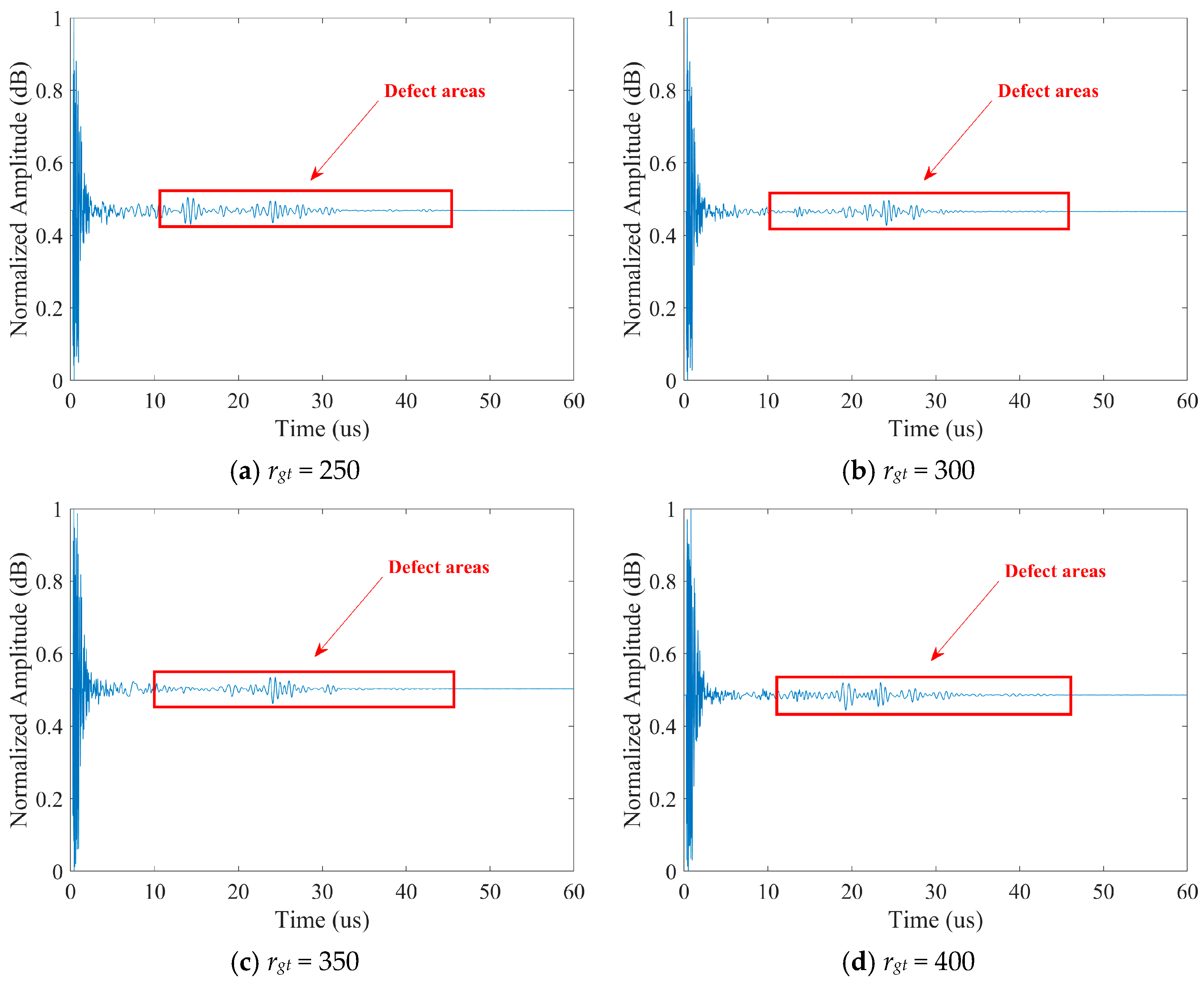
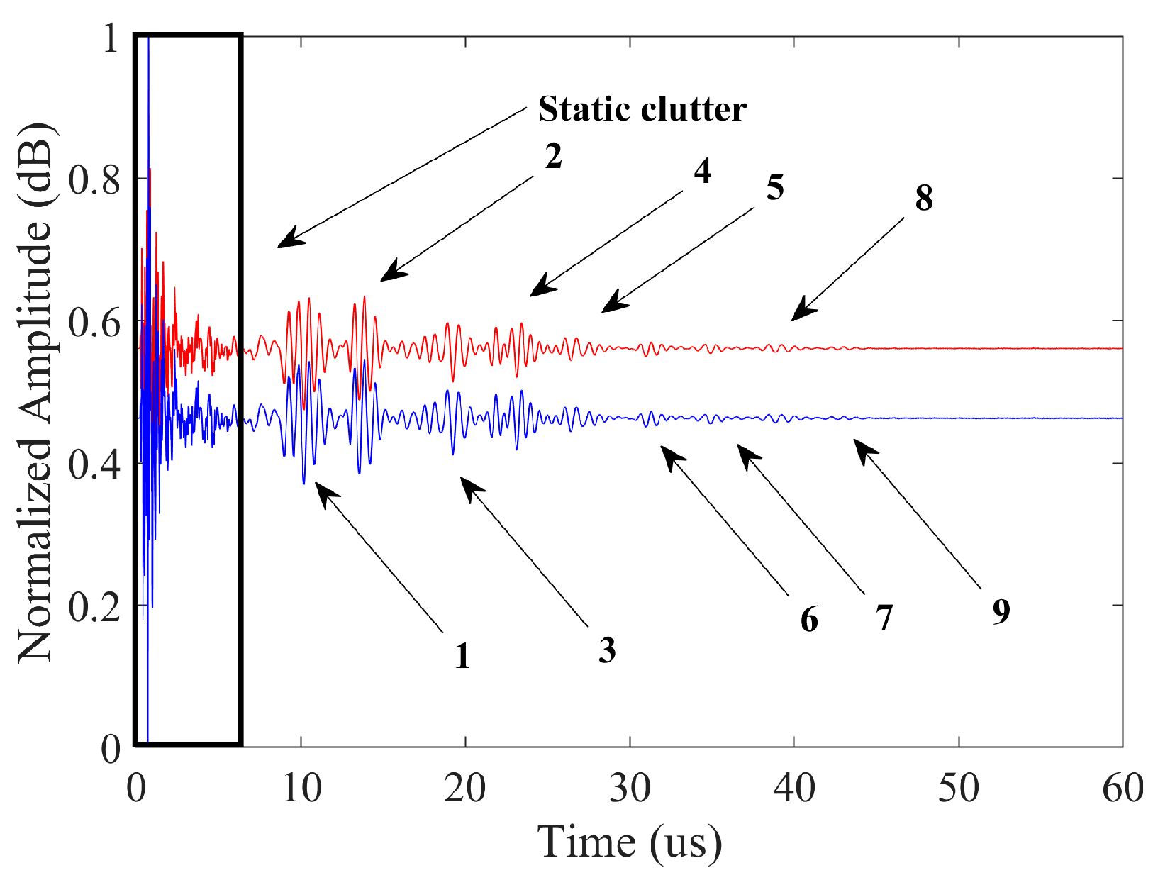
3.1. A-Scan Signal Analysis
3.2. STSVD Signal Filtering
4. Results and Discussion
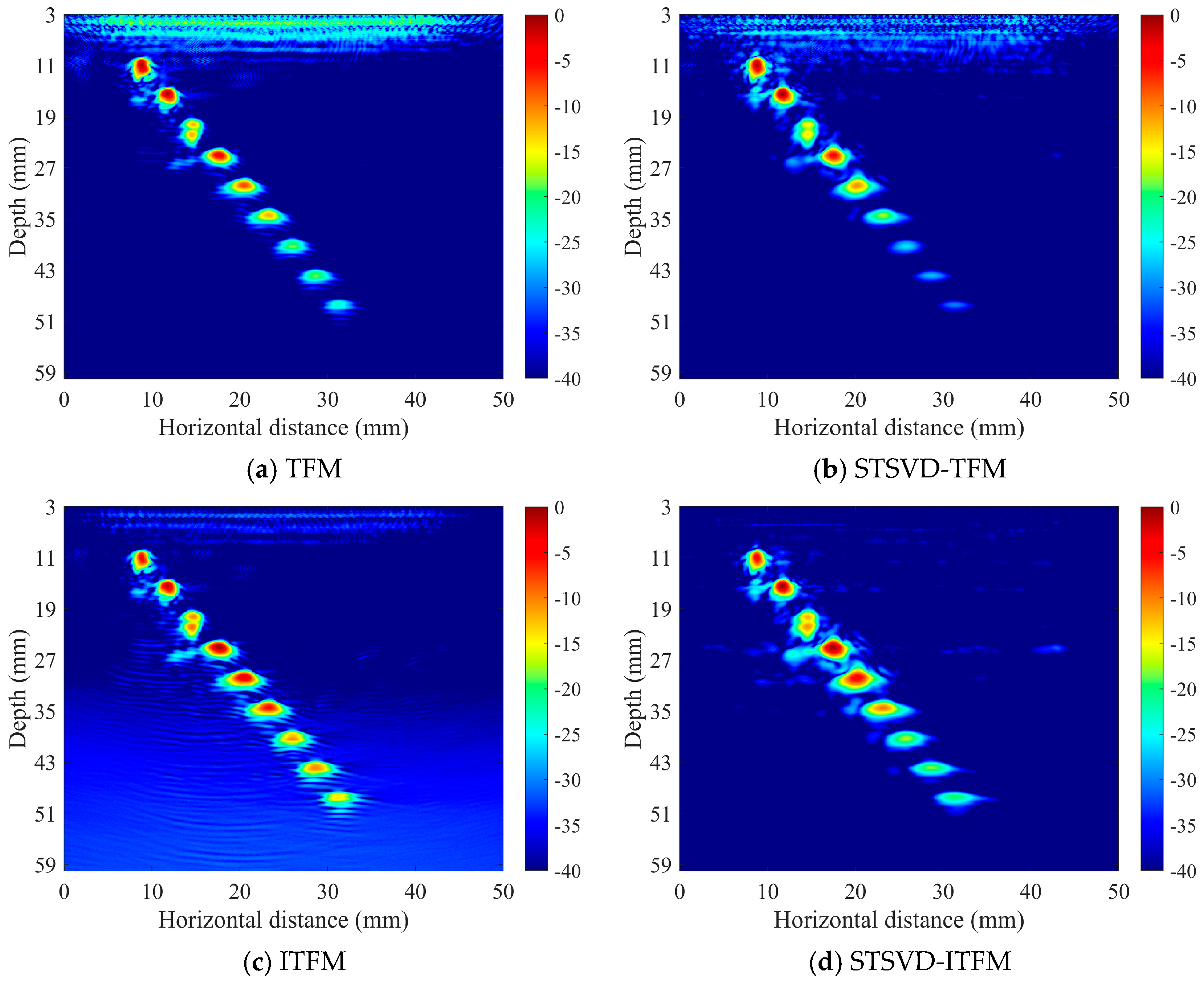
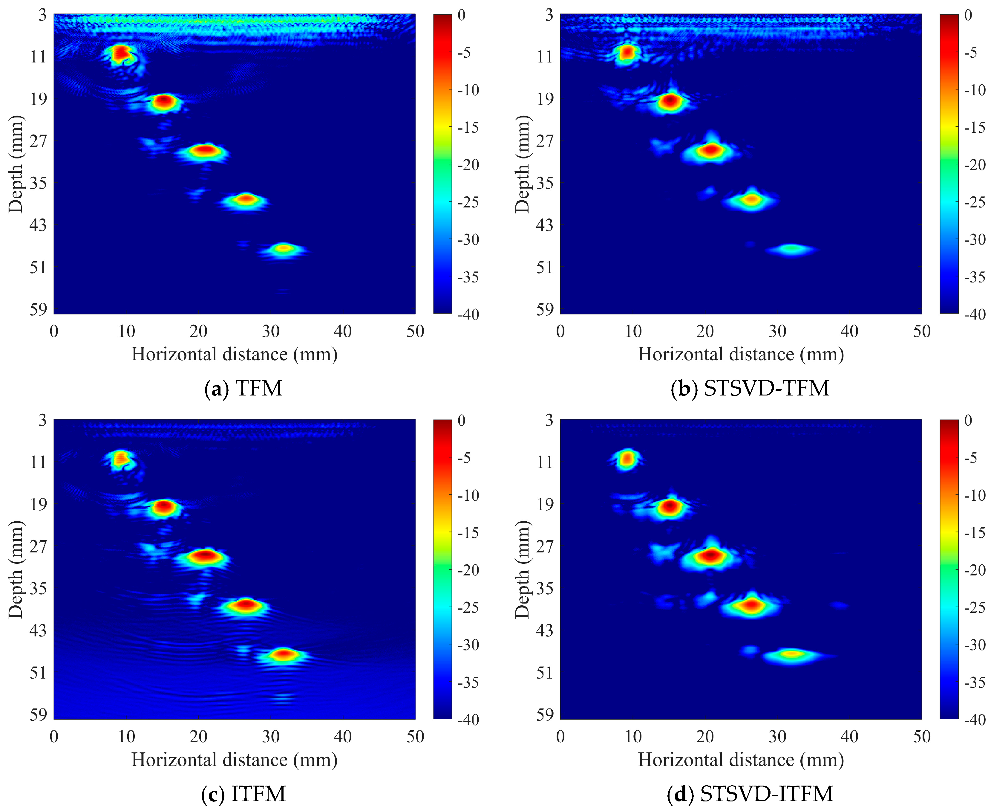
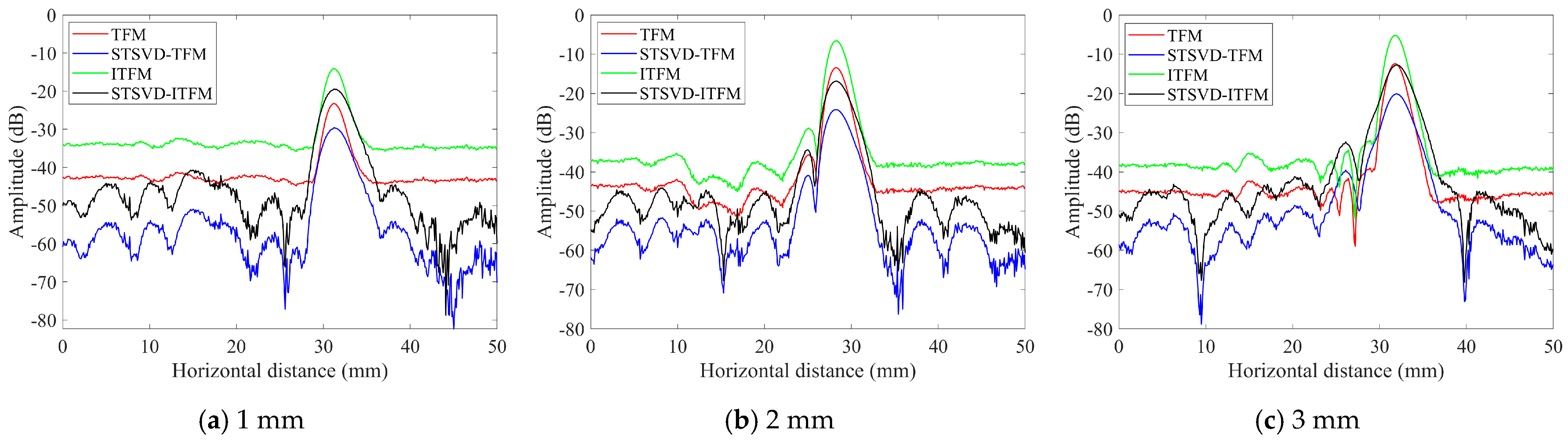
4.1. Comparison of Imaging Results
4.2. Analysis of Relevant Imaging Data
5. Conclusions
Author Contributions
Funding
Data Availability Statement
Conflicts of Interest
References
- Gong, Y.; Wang, S.-H.; Zhang, Z.-Y.; Yang, X.-L.; Yang, Z.-G.; Yang, H.-G. Degradation of Sunlight Exposure on the High-Density Polyethylene (HDPE) Pipes for Transportation of Natural Gases. Polym. Degrad. Stab. 2021, 194, 109752. [Google Scholar] [CrossRef]
- Guo, H.; Rinaldi, R.G.; Tayakout, S.; Broudin, M.; Lame, O. The Correlation between the Mixed-Mode Oligo-Cyclic Loading Induced Mechanical and Microstructure Changes in HDPE. Polymer 2021, 224, 123706. [Google Scholar] [CrossRef]
- Kim, J.-S.; Oh, Y.-J.; Choi, S.-W.; Jang, C. Investigation on the Thermal Butt Fusion Performance of the Buried High Density Polyethylene Piping in Nuclear Power Plant. Nucl. Eng. Technol. 2019, 51, 1142–1153. [Google Scholar] [CrossRef]
- Pokharel, P.; Kim, Y.; Choi, S. Microstructure and Mechanical Properties of the Butt Joint in High Density Polyethylene Pipe. Int. J. Polym. Sci. 2016, 2016, 6483295. [Google Scholar] [CrossRef]
- Lai, H.; Fan, D.; Liu, K. The Effect of Welding Defects on the Long-Term Performance of HDPE Pipes. Polymers 2022, 14, 3936. [Google Scholar] [CrossRef] [PubMed]
- Shi, J.; Feng, Y.; Tao, Y.; Guo, W.; Yao, R.; Zheng, J. Evaluation of the Seismic Performance of Butt-Fusion Joint in Large Diameter Polyethylene Pipelines by Full-Scale Shaking Table Test. Nucl. Eng. Technol. 2023, 55, 3342–3351. [Google Scholar] [CrossRef]
- Egerton, J.S.; Lowe, M.J.S.; Huthwaite, P.; Halai, H.V. Ultrasonic Attenuation and Phase Velocity of High-Density Polyethylene Pipe Material. J. Acoust. Soc. Am. 2017, 141, 1535–1545. [Google Scholar] [CrossRef] [PubMed]
- Lai, H.S.; Tun, N.N.; Yoon, K.B.; Kil, S.H. Effects of Defects on Failure of Butt Fusion Welded Polyethylene Pipe. Int. J. Press. Vessel. Pip. 2016, 139–140, 117–122. [Google Scholar] [CrossRef]
- Djebli, A.; Bendouba, M.; Aid, A.; Talha, A.; Benseddiq, N.; Benguediab, M. Experimental Analysis and Damage Modeling of High-Density Polyethylene under Fatigue Loading. Acta Mech. Solida Sin. 2016, 29, 133–144. [Google Scholar] [CrossRef]
- Majid, F.; Elghorba, M. HDPE Pipes Failure Analysis and Damage Modeling. Eng. Fail. Anal. 2017, 71, 157–165. [Google Scholar] [CrossRef]
- Ur Rahman, M.S.; Haryono, A.; Abou-Khousa, M.A. Microwave Non-Destructive Evaluation of Glass Reinforced Epoxy and High Density Polyethylene Pipes. J. Nondestruct. Eval. 2020, 39, 26. [Google Scholar] [CrossRef]
- Zheng, J.; Zhang, Y.; Hou, D.; Qin, Y.; Guo, W.; Zhang, C.; Shi, J. A Review of Nondestructive Examination Technology for Polyethylene Pipe in Nuclear Power Plant. Front. Mech. Eng. 2018, 13, 535–545. [Google Scholar] [CrossRef]
- Frederick, C.; Porter, A.; Zimmerman, D. High-Density Polyethylene Piping Butt-Fusion Joint Examination Using Ultrasonic Phased Array. J. Press. Vessel. Technol. 2010, 132, 051501. [Google Scholar] [CrossRef]
- Lacaze, B. Random Propagation Times for Ultrasonics through Polyethyilene. Ultrasonics 2021, 111, 106313. [Google Scholar] [CrossRef] [PubMed]
- Zheng, J.; Hou, D.; Guo, W.; Miao, X.; Zhou, Y.; Shi, J. Ultrasonic Inspection of Electrofusion Joints of Large Polyethylene Pipes in Nuclear Power Plants. J. Press. Vessel. Technol. 2016, 138, 060908. [Google Scholar] [CrossRef]
- Qin, Y.; Shi, J.; Zheng, J.; Hou, D.; Guo, W. An Improved Phased Array Ultrasonic Testing Technique for Thick-Wall Polyethylene Pipe Used in Nuclear Power Plant. J. Press. Vessel. Technol. 2019, 141, 041403. [Google Scholar] [CrossRef]
- Behravan, A.; Tran, T.Q.; Li, Y.; Davis, M.; Shaikh, M.S.; DeJong, M.M.; Hernandez, A.; Brand, A.S. Field Inspection of High-Density Polyethylene (HDPE) Storage Tanks Using Infrared Thermography and Ultrasonic Methods. Appl. Sci. 2023, 13, 1396. [Google Scholar] [CrossRef]
- Holmes, C.; Drinkwater, B.W.; Wilcox, P.D. Post-Processing of the Full Matrix of Ultrasonic Transmit–Receive Array Data for Non-Destructive Evaluation. NDT E Int. 2005, 38, 701–711. [Google Scholar] [CrossRef]
- Lopez Villaverde, E.; Robert, S.; Prada, C. Ultrasonic Imaging in Highly Attenuating Materials With Hadamard Codes and the Decomposition of the Time Reversal Operator. IEEE Trans. Ultrason. Ferroelectr. Freq. Control. 2017, 64, 1336–1344. [Google Scholar] [CrossRef]
- Zong, S.; Wang, S.; Luo, Z.; Wu, X.; Zhang, H.; Ni, Z. Robust Damage Detection and Localization Under Complex Environmental Conditions Using Singular Value Decomposition-Based Feature Extraction and One-Dimensional Convolutional Neural Network. Chin. J. Mech. Eng. 2023, 36, 61. [Google Scholar] [CrossRef]
- Liu, C.; Harley, J.B.; Bergés, M.; Greve, D.W.; Oppenheim, I.J. Robust Ultrasonic Damage Detection under Complex Environmental Conditions Using Singular Value Decomposition. Ultrasonics 2015, 58, 75–86. [Google Scholar] [CrossRef] [PubMed]
- Xu, L.; Chatterton, S.; Pennacchi, P. Rolling Element Bearing Diagnosis Based on Singular Value Decomposition and Composite Squared Envelope Spectrum. Mech. Syst. Signal. Pract. 2021, 148, 107174. [Google Scholar] [CrossRef]
- Shahjahan, S.; Rupin, F.; Aubry, A.; Derode, A. Evaluation of a Multiple Scattering Filter to Enhance Defect Detection in Heterogeneous Media. J. Acoust. Soc. Am. 2017, 141, 624–640. [Google Scholar] [CrossRef] [PubMed]
- Cunningham, L.J.; Mulholland, A.J.; Tant, K.M.M.; Gachagan, A.; Harvey, G.; Bird, C. The Detection of Flaws in Austenitic Welds Using the Decomposition of the Time-Reversal Operator. Proc. R. Soc. A—Math. Phys. Eng. Sci. 2016, 472, 20150500. [Google Scholar] [CrossRef] [PubMed]
- Zhang, Y.; Gao, X.; Zhang, J.; Jiao, J. An Ultrasonic Reverse Time Migration Imaging Method Based on Higher-Order Singular Value Decomposition. Sensors 2022, 22, 2534. [Google Scholar] [CrossRef] [PubMed]
- Rao, J.; Zeng, L.; Liu, M.; Fu, H. Ultrasonic Defect Detection of High-Density Polyethylene Pipe Materials Using FIR Filtering and Block-Wise Singular Value Decomposition. Ultrasonics 2023, 134, 107088. [Google Scholar] [CrossRef] [PubMed]
- Demene, C.; Deffieux, T.; Pernot, M.; Osmanski, B.-F.; Biran, V.; Gennisson, J.-L.; Sieu, L.-A.; Bergel, A.; Franqui, S.; Correas, J.-M.; et al. Spatiotemporal Clutter Filtering of Ultrafast Ultrasound Data Highly Increases Doppler and fUltrasound Sensitivity. IEEE Trans. Med. Imaging 2015, 34, 2271–2285. [Google Scholar] [CrossRef] [PubMed]
- Al Mukaddim, R.; Weichmann, A.M.; Mitchell, C.C.; Varghese, T. Enhancement of In Vivo Cardiac Photoacoustic Signal Specificity Using Spatiotemporal Singular Value Decomposition. J. Biomed. Opt. 2021, 26, 046001. [Google Scholar] [CrossRef] [PubMed]
- Baranger, J.; Arnal, B.; Perren, F.; Baud, O.; Tanter, M.; Demene, C. Adaptive Spatiotemporal SVD Clutter Filtering for Ultrafast Doppler Imaging Using Similarity of Spatial Singular Vectors. IEEE Trans. Med. Imaging 2018, 37, 1574–1586. [Google Scholar] [CrossRef]
- Rao, J.; Qiu, H.; Teng, G.; Al Mukaddim, R.; Xue, J.; He, J. Ultrasonic Array Imaging of Highly Attenuative Materials with Spatio-Temporal Singular Value Decomposition. Ultrasonics 2022, 124, 106764. [Google Scholar] [CrossRef]
- Zhang, H.; Bai, B.; Zheng, J.; Zhou, Y. Optimal Design of Sparse Array for Ultrasonic Total Focusing Method by Binary Particle Swarm Optimization. IEEE Access 2020, 8, 111945–111953. [Google Scholar] [CrossRef]
- Zhu, W.; Xiang, Y.; Zhang, H.; Cheng, Y.; Fan, G.; Zhang, H. Research on Ultrasonic Sparse DC-TFM Imaging Method of Rail Defects. Measurement 2022, 200, 111690. [Google Scholar] [CrossRef]
- Hu, H.; Du, J.; Xu, N.; Jeong, H.; Wang, X. Ultrasonic Sparse-TFM Imaging for a Two-Layer Medium Using Genetic Algorithm Optimization and Effective Aperture Correction. NDT E Int. 2017, 90, 24–32. [Google Scholar] [CrossRef]
- Teng, D.; Liu, L.; Xiang, Y.; Xuan, F.-Z. An Optimized Total Focusing Method Based on Delay-Multiply-and-Sum for Nondestructive Testing. Ultrasonics 2023, 128, 106881. [Google Scholar] [CrossRef]


| Associated Acquired and Processed Ultrasonic Parameters | Value |
|---|---|
| Number of active array elements in the probe | 64 |
| The active array element width | 0.6 mm |
| The active array element pitch | 0.75 mm |
| Center frequency | 2.25 MHz |
| Sampling frequency | 62.5 MHz |
| Excitation voltage | 100.0 V |
| The signal pulse width | 300.0 ns |
| Sound velocity | 2300.0 m/s |
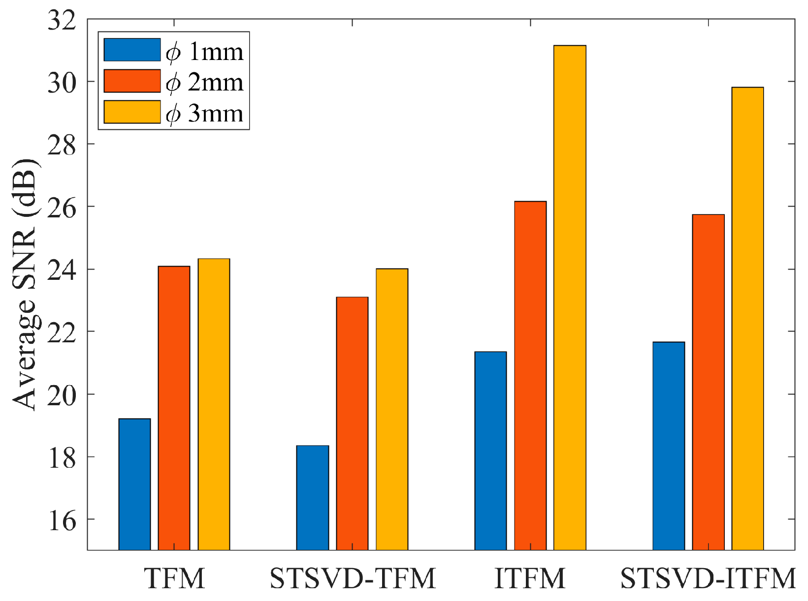
| Type of Defect | Average SNR (dB) | |
|---|---|---|
| 1 mm | 19.20 | TFM |
| 18.36 | STSVD-TFM | |
| 21.36 | ITFM | |
| 21.66 | STSVD-ITFM | |
| 2 mm | 24.09 | TFM |
| 23.11 | STSVD-TFM | |
| 26.16 | ITFM | |
| 25.75 | STSVD-ITFM | |
| 3 mm | 24.33 | TFM |
| 24.01 | STSVD-TFM | |
| 31.14 | ITFM | |
| 29.81 | STSVD-ITFM |
| Actual Depth (mm) | Measured Depth (mm) | ||||
|---|---|---|---|---|---|
| TFM | STSVD-TFM | ITFM | STSVD-ITFM | ||
| no. 1 | 10.00 | 11.10 | 11.10 | 11.10 | 11.00 |
| no. 2 | 15.00 | 15.40 | 15.40 | 15.40 | 15.40 |
| no. 3 | 20.00 | 21.10 | 21.15 | 21.10 | 21.05 |
| no. 4 | 25.00 | 25.10 | 25.10 | 25.10 | 25.00 |
| no. 5 | 30.00 | 29.80 | 29.80 | 29.80 | 29.90 |
| no. 6 | 35.00 | 34.60 | 34.50 | 34.60 | 34.60 |
| no. 7 | 40.00 | 39.50 | 39.40 | 39.50 | 39.40 |
| no. 8 | 45.00 | 44.10 | 44.00 | 44.10 | 44.20 |
| no. 9 | 50.00 | 48.30 | 48.50 | 48.30 | 48.50 |
| Average error (mm) | 0.71 | 0.73 | 0.71 | 0.67 | |
| Actual Depth (mm) | Measured Depth (mm) | ||||
|---|---|---|---|---|---|
| TFM | STSVD-TFM | ITFM | STSVD-ITFM | ||
| no. 1 | 10.00 | 10.60 | 10.90 | 10.60 | 10.40 |
| no. 2 | 15.00 | 15.00 | 15.30 | 15.00 | 15.00 |
| no. 3 | 20.00 | 19.70 | 19.70 | 19.70 | 19.80 |
| no. 4 | 25.00 | 24.40 | 24.40 | 24.40 | 24.40 |
| no. 5 | 30.00 | 29.20 | 29.20 | 29.20 | 29.40 |
| no. 6 | 35.00 | 33.80 | 33.90 | 33.90 | 33.90 |
| no. 7 | 40.00 | 38.50 | 38.50 | 38.50 | 38.40 |
| no. 8 | 45.00 | 43.30 | 43.30 | 43.30 | 43.30 |
| no. 9 | 50.00 | 48.00 | 48.00 | 48.00 | 48.10 |
| Average error (mm) | 0.96 | 1.02 | 0.96 | 0.92 | |
| Actual Depth (mm) | Measured Depth (mm) | ||||
|---|---|---|---|---|---|
| TFM | STSVD-TFM | ITFM | STSVD-ITFM | ||
| no. 1 | 10.00 | 10.10 | 10.30 | 10.50 | 10.40 |
| no. 2 | 20.00 | 19.20 | 19.30 | 19.20 | 19.50 |
| no. 3 | 30.00 | 28.70 | 28.80 | 28.70 | 28.80 |
| no. 4 | 40.00 | 38.10 | 38.20 | 38.10 | 38.20 |
| no. 5 | 50.00 | 47.50 | 47.60 | 47.50 | 47.70 |
| Average error (mm) | 1.32 | 1.28 | 1.4 | 1.24 | |
Disclaimer/Publisher’s Note: The statements, opinions and data contained in all publications are solely those of the individual author(s) and contributor(s) and not of MDPI and/or the editor(s). MDPI and/or the editor(s) disclaim responsibility for any injury to people or property resulting from any ideas, methods, instructions or products referred to in the content. |
© 2024 by the authors. Licensee MDPI, Basel, Switzerland. This article is an open access article distributed under the terms and conditions of the Creative Commons Attribution (CC BY) license (https://creativecommons.org/licenses/by/4.0/).
Share and Cite
Zhang, H.; Wang, Q.; Zhou, J.; Wu, L.; Xu, W.; Wang, H. High-Density Polyethylene Pipe Butt-Fusion Joint Detection via Total Focusing Method and Spatiotemporal Singular Value Decomposition. Processes 2024, 12, 1267. https://doi.org/10.3390/pr12061267
Zhang H, Wang Q, Zhou J, Wu L, Xu W, Wang H. High-Density Polyethylene Pipe Butt-Fusion Joint Detection via Total Focusing Method and Spatiotemporal Singular Value Decomposition. Processes. 2024; 12(6):1267. https://doi.org/10.3390/pr12061267
Chicago/Turabian StyleZhang, Haowen, Qiang Wang, Juan Zhou, Linlin Wu, Weirong Xu, and Hong Wang. 2024. "High-Density Polyethylene Pipe Butt-Fusion Joint Detection via Total Focusing Method and Spatiotemporal Singular Value Decomposition" Processes 12, no. 6: 1267. https://doi.org/10.3390/pr12061267