Abstract
An algorithm based on continuous measurement of multiphase flows of oil well production has been designed to improve the efficiency of the technical control of oil production processes in the field. Separation-free, non-contact measurement of multiphase flows of oil well products allows increasing the efficiency of managing oil production processes in the field. Monitoring the current density using radioisotope measuring transducers (RMTs) allows obtaining information about the structure of the flow in the form of the distribution of gas inclusions and the speed of movement of liquid and gas in a two-phase flow. Fluid velocity measurement is based on digital processing of RMT signals, applying a continuous or discrete undecimated wavelet transform to them, and assessing the cross-correlation of wavelet coefficients in individual subspaces of the wavelet decomposition. The cross-correlation coefficients of two RMT signals located at a base distance, calculated in the subspaces of the wavelet decomposition, characterize the speed of movement of gas bubbles of different sizes in a vertical pipe. The measurement assumes that the velocity of the liquid phase of the oil flow in a vertical pipe mainly corresponds to the velocity of small bubbles. This speed should be determined by the maximum cross-correlation of wavelet coefficients in the corresponding decomposition subspace. Computer modeling made it possible to evaluate the characteristics of the algorithm for controlling the speed of liquid movement in the gas–liquid flow of oil well products and determine the mass flow rate of the liquid and the relative value of the gas content. The implementation of the algorithm in a multi-channel version of the device allows monitoring an entire cluster of wells in the field.
1. Introduction
An important part of oil production management is measuring the current characteristics of the gas–liquid flow and optimizing the operating mode of oil wells. For engineering tasks of process control, a measurement error of 5–10% is quite acceptable. To measure the flow rate of oil and gas production wells by the mass of crude oil and the volume of free petroleum gas, a separation measuring unit [1] is often used, the principle of which is to separate the oil and gas mixture into a liquid phase containing crude oil and a gas phase. After separation, the mass of crude oil and the volume of free petroleum gas are measured. Separation plants have large metal separation tanks. Therefore, the disadvantages of separation plants include their high metal consumption and cost, operation in an aggressive environment and high pressure. Separation units are usually used as a part of groups serving several wells at once, and measurements are carried out periodically. Therefore, multiphase radioisotope flow meters are promising tools for continuously measuring well fluid flow rates without phase separation and without interfering with the flow. In addition, radioisotope flow meters have no moving parts, are highly reliable, have a wide operating range, provide minimal pressure loss, are resistant to contamination, and have a high measurement speed without intrusion into the flow. Radioisotope measurements do not involve sample selection [2,3,4].
Multiphase flow meters used in oil production process control systems use different physical principles. For example, in [3], the authors propose a combined measurement system for monitoring the three-phase flow of oil well production, based on the ultrasonic effect using a fiber-bioptic sensor. The authors of [5] proposed a new technique for measuring three-phase well flow based on measurements of sound speed at different locations in the well and an intelligent dynamic monitoring method using machine learning. The three-phase flow prediction model discussed in [6] is based on the attenuation of ultrasound transmission in certain flow patterns. Several publications have proposed changing the flow structure to obtain control results for production processes. For example, the authors of [4,6] have proposed to use a density meter in conjunction with a Venturi-type flow meter to measure the flow rate of oil and gas in a pipeline. At the same time, the developers of a multiphase flow meter [7] used a mixture homogenizer, a Coriolis flow meter, and an infrared-fractional counter, and intelligent processing of control results. Ultrasonic methods include dynamic monitoring of low-yield gas wells based on ultrasonic Doppler logging and a machine-learning algorithm [8].
Nuclear magnetic resonance technologies have been applied to a multiphase flow meter [9], allowing designers to control the composition and velocities of individual phases for multiphase flow.
The most promising for use in the oil and gas industry are radioisotope methods capable of performing non-contact, separation-free monitoring of multiphase flows under extreme operating conditions. Several scientific studies have been devoted to the development of radioisotope monitoring systems. For technological control of heavy oil production processes, a multiphase flow meter based on neutron activation analysis has been proposed in [10]. Preliminary studies have shown that neutron activation analysis methods make it possible to determine the content of oil, water, and gas, the ratio of sulfur and chlorine, the level of water cut in oil, and calculate the speed of phase movement. The use of the gamma radiation attenuation effect and the artificial intelligence method for measuring the density of a multiphase flow, determining the type of flow regime, and calculating the volumetric gas content in a two-phase flow are discussed in [11]. The production system proposed by the authors includes a gamma radiation source containing radioisotopes of barium-133 and cesium-137. When continuing their research, these authors proposed using X-ray sources instead of radioisotopes [12], which allowed them to achieve some improvement in the accuracy of measurements. The comparison of the two methods was carried out using Monte Carlo simulation and the use of a multilayer perceptron to determine the flow rates of the liquid and gas phases of the flow. It seems important to study the influence of liquid density and viscosity on the characteristics of a radioisotope multiphase flow meter, which was carried out in [13]. The formation of paraffins in some fields is a complex problem in oil production, since the deposition of paraffins negatively affects the operation of production wells. Paraffins deposited on the inner surface of the pipe reduce the volume of flowing liquid. Performing calibration on an empty pipe can significantly reduce the influence of paraffins [14].
Radioisotope systems make it possible to control the deposition of paraffins on the pipe walls. The authors of publication [15] consider the issues of stable oil production from paraffinic oil fields. Controlling three separate flow phase velocities is complex and requires measuring the speed of each phase and the magnitude of each phase’s relative contribution to the flow. Measurements can be performed under different flow regimes of the gas–liquid mixture in a vertical pipe: bubble, slug, dispersed annular. At low values of gas content, the flow of the two-phase mixture corresponds to the bubble regime. A special class of equipment is formed by correlation flow meters based on the calculation of the autocorrelation function, structure function or cross-correlation function of the flow density. The correlation method of flow control is complicated by the fact that in typical oil well production flows, liquid and gas have different velocities. The correlation method of flow control is complicated by the fact that in typical oil well production flows, liquid and gas inclusions of various sizes have different velocities. Larger bubbles move faster, smaller ones move slower. Therefore, without preliminary signal processing, gas bubbles cannot serve as flow marks suitable for use in the correlation method.
Autocorrelation-based flow meters that process single-point flow density signals are forced to calculate the derivative of the autocorrelation or structure function to amplify the effect of density fluctuations caused by small gas inclusions. Correlation flow meters are based on calculating the cross-correlation of the signals from density meters located at a fixed distance at two points along the pipe. For example, article [16] shows that the speed of movement of relatively large gas inclusions exceeds the speed of liquid movement due to the predominance of the Archimedes force over the friction force. At the same time, small bubbles move at a speed close to the speed of the liquid. Therefore, they can be flowing labels. Fluctuations in the density of the mixture depend both on the speed of the liquid and on the structure of the flow. It becomes relevant to isolate from the density fluctuation signal the component that characterizes the speed of fluid movement. An analytical review of methods for measuring two-phase flows was carried out in [17,18].
Radioisotope methods for monitoring oil well performance have many advantages [19,20]. They allow non-contact measurements without penetration into the flow, allow the deposition of paraffins on the walls of pipes, do not require separation of flow phases, do not introduce delays, and operate in real time. Devices using the radioisotope method can operate in extreme conditions; they have no moving parts, which means they have increased reliability, do not require constant human presence, and therefore are promising means of monitoring oil production processes. One of the most important challenges for these devices is the development of more advanced algorithm methods that improve the manufacturability of industrial processes for monitoring oil field performance. The objective of this research is to improve the method of signal processing, the current density of the two-phase flow generated by the RMT, as well as the development of an algorithm and program that are based on the mutual correlation of two RMT signals located at a base distance. The algorithm must be adjusted to the structure of a two-phase oil and gas flow, which has different speeds of movement of liquid and gas inclusions of different sizes.
2. Materials and Methods
2.1. Radioisotope Multiphase Flow Meter
Gamma rays emitted by a Cs-137 radiation source pass through a two-phase flow and are partially absorbed by the liquid part of the flow. The radiation detector is built on a scintillator, a NaJ(Tl) crystal, a photomultiplier, and an electronic unit designed to record the number and power of pulses arriving during a given time interval τ (in particular τ = 0.2 ms). The RMT includes a radiation source and receiver for continuous monitoring of the multiphase flow density with a time interval τ and a computing device designed to analyze the time series of density changes and calculate the speed and average flow density. The RMT is configured to register pulses of a certain energy range. For multiphase flow, several regions of the energy spectrum of the gamma radiation source can be used. Pulse sequences received through high-energy 660 keV pulse detection channels are generated by a direct photon flux, while lower-energy 30 keV pulses are generated by scattered radiation. The information signal characterizes the density of a moving multiphase flow containing liquid and gaseous components.
Figure 1 shows the appearance and diagram of the RMT, (a)—appearance of the device, (b)—block diagram of the device, (c)—structure of the oil and gas flow. Sources of collimated gamma radiation Sz-137 (1,2) are located at a base distance on one side of the tube, and scintillation radiation detectors (3,4) are located on the opposite side. Detector blocks register gamma quanta and generate pulses, the amplitude of which is proportional to the energy of the quanta. Using a given threshold, the pulses are divided into two channels of direct and scattered radiation. Pulses whose amplitude is below the threshold form a channel of scattered radiation; the registration rate of these pulses depends on the average density of the two-phase flow in the pipe (5). High-amplitude pulses characterize flux density fluctuations in a narrow flux tube.
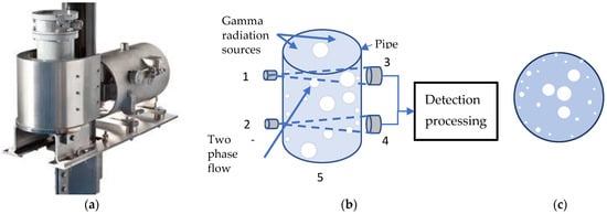
Figure 1.
Radioisotope converter, (a) appearance of the radioisotope converter, (b) structure of the radioisotope converter, (c) gas–liquid flow in the cross section of a vertical pipe.
To effectively control the production process, it is necessary to separately measure the velocity of the liquid and gaseous phases of the flow and determine the relative content of each phase in the flow. It should be noted that measuring the speed of movement of individual flow phases is a more complex task [21,22].
The liquid in the pipe absorbs or scatters gamma rays emanating from two radiation sources; the presence of bubbles reduces both absorption and scattering. According to the flow structure, the bubbles in the pipe are located randomly and have different diameters. Flow control assumes that small bubbles are markers that measure the speed of fluid movement. Gas inclusions of all sizes determine the average flow density.
The main difficulty is that in a gas–liquid flow there is a relative movement of phases due to the difference in their densities and viscosities, surface tension at the phase boundary, and the slope of the pipeline. When a gas–liquid mixture moves through vertical pipes, the gas will either be randomly distributed in the liquid in the form of small bubbles or move in the form of separate gas accumulations in the center of the pipe [23].
When high-viscosity oil rises, friction plays a significant role, and the emulsion structure of the flow changes little. At the same time, friction when lifting low-viscosity oil is lower, and the flow structure can change. In any case, bubbles of small diameter, grouped at the periphery of the flow near the pipe walls, move at the speed of the liquid flow. Therefore, fluctuations in the RMT signal caused by the movement of small bubbles can serve as flow markers. To separate the flow marks and calculate the cross-correlation between the density fluctuations present in the two receiver signals, it is advisable to use multilevel wavelet analysis.
The attenuation of the intensity of a beam of γ-quanta, when interacting with atoms of a substance, depends on the linear attenuation coefficient, the density of the oil, and the thickness of the absorbing layer according to Bouguer’s law:
where is the count rate of gamma rays of direct radiation obtained when calibrating the device with an empty pipe, is the density of the absorber obtained during the measurement, is the linear absorption coefficient, depending on the properties of the oil, and is the thickness of the absorber layer, which depends on the presence of free gas in the pipe.
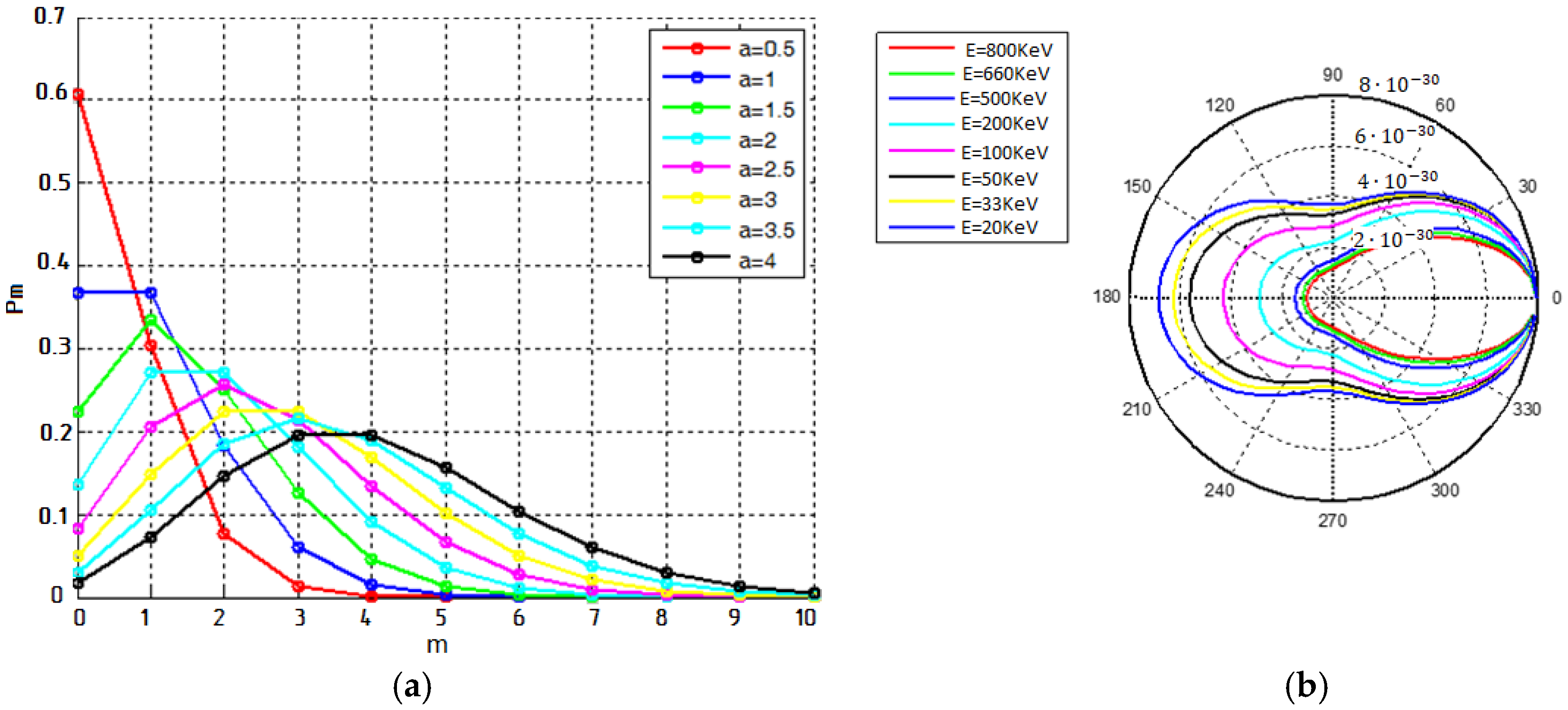
The number of gamma rays emitted by the source is distributed according to Poisson’s law, which is characterized by the mathematical expectation , variation , skewness coefficient , and kurtosis coefficient . Figure 2a shows the distributions corresponding to a different parameter .

Figure 2.
Physical foundations of an RMT. (a) Distributions corresponding to different parameter . (b) Differential Compton scattering cross section.
The nature of the interaction of photons with matter depends on the substance and the physical law of scattering. The mathematical model is based on the Klein–Nishina–Tamm relation characterizing the interaction of photons with matter. The processes of interaction of gamma radiation with matter, depending on the radiation energy, are divided into the photoelectric effect, scattering without a change in wavelength (Thomson scattering), scattering with a change in wavelength (Compton effect), and pair formation [24,25].
The Cs137 radiation source has energy . In the photon radiation energy range of 0.2–5.0 MeV, the Compton effect predominates at any atomic number of the medium Z, and its role increases as Z decreases. The Compton effect is characterized by a change in the frequency of photons when they are scattered by electrons of the outer atomic shells of a substance surfac. During Compton scattering, a photon deviates by a certain angle from its original direction of motion. Part of its energy is transferred to an electron, which becomes a recoil electron.
The differential cross section for Compton scattering per electron, per unit solid angle, is expressed by the Klein–Nishina–Tamm formula, which determines the probability of photon scattering at solid angle
where is the classical electron radius; is the electron charge; is the electron mass; is the speed of light; is the fine structure constant; is gamma quantum energy; —electron mass; is scattering angle (the angle between the directions of the primary and scattered photons).
The intensity of scattered photon radiation that depends on the intensity of primary radiation , the scattering angle (the angle between the directions of the primary and scattered photons) at a distance from the scattering electron is expressed by the following relation:
where (cm2) is the Compton cross section, is electron concentration in the scattering layer, is the effective atomic number of the substance, is the fine structure constant, kg is electron rest mass, m/c is the speed of light, and Joule is electron rest energy. Figure 2b shows a differential Compton scattering cross section.
2.2. Wavelet Cross-Correlation Based on Continuous Wavelet Transform
Multilevel wavelet analysis of RMT signals allows us to determine the structure of a two-phase gas–liquid flow by representing the signals in wavelet subspaces. The distribution of signals from two RMTs in each space characterizes the patterns of movement of flow inhomogeneities, and the correlation between signals in each space characterizes the relative speeds of movement of the structural elements of the flow [26]. In article [27], the authors discuss the results of applied research work on the use of the continuous wavelet transform and discrete orthogonal wavelet transform in fluid mechanics. Cross-correlation signal processing has many applications in engineering, including in problems of measuring velocity in multiphase flows [28,29]. Therefore, the task of improving algorithms for measuring the flow rate of a multiphase oil and gas flow when monitoring technological processes for obtaining oil well production seems promising.
The short-time Fourier transform (STFT) allows you to analyze the structure of a two-phase flow in the time–frequency space and determine the relative displacement of frequency components over time as the flow moves. Since the flow is not characterized by harmonic properties, compact wavelet functions are more suitable for analyzing its properties. The continuous wavelet transform (CWT) is often used to extract useful features of signals with low signal-to-noise ratios, characteristic of RMT signals that contain non-additive Poisson noise. To study the time relationship of two signals separately for each scale of gas inclusions, CWT is more suitable, since it allows one to observe the time dependences of signals at higher frequencies with higher resolution. The STFT has the same time resolution at all frequencies. The CWT of signals, represented in time scale coordinates, is a scalogram.
To a discrete signal RMT denoted here by where is discrete time, a scaled and translated wavelet function is defined as a convolution of signal:
where is the sampling interval, is the scaled and shifted mother wavelet function, and is the complex conjugate wavelet function. Wavelet coefficients are calculated at each scale for each time index . Wavelet coefficients represent projections of the signal onto the time and scale plane. The mother wavelet is a function that is a prototype for the functions used in the wavelet transform. All wavelets are generated by rescaling and shifting the mother wavelet. Scale can be considered as an analogue of frequency in the STFT. Smoothing wavelet coefficients over time and over adjacent scales makes it possible to suppress random noise present in the signals. By smoothing the wavelet spectrum over time, the significance of wavelet power peaks can be increased. In this case, the correlation appears to lengthen in time as the scale increases and the wavelet function expands. By calculating the weighted sum of wavelet coefficients over adjacent scales, it is possible to reduce the fluctuations of the wavelet transform result in the scale domain.
Wavelet decomposition is usually performed using a more efficient algorithm that uses the convolution theorem. Wavelet coefficients are calculated as the inverse Fourier transform of the product of the Fourier image of the signal frame and the Fourier image of the wavelet function :
where is the operator of the inverse discrete Fourier transform in the scale .
The algorithm for calculating the correlation of signals in CWT subspaces is applied to two discrete centered signals and , coming from RMTs located at the base distance.
For each frame of length 1024 samples containing signals and , we calculated the DFT:
where 1 denotes the frequency index.
Wavelet decomposition parameters: minimum scale and maximum level of expansion for specific levels decomposition and scale vector . Pseudo-frequencies are related to the scale : considering the Fourier multiplier , which depends on the type of wavelet.
To analyze RMT signals, a continuous Morlet wavelet was chosen, with the frequency parameter The discrete Fourier transform (DFT) for the analytical Morlet wavelet is determined by the following formula:
Continuous non-orthogonal wavelets are effective for the analysis of signals: the Morlet complex wavelet, the Pole complex wavelet, and the real Gaussian difference wavelet. Mathematical expression (5) contains the Heaviside function . Normalization of wavelet coefficients is performed on each decomposition scale:
Element-wise multiplication in the Fourier domain of the analyzed signal and the shifted and scaled wavelet functions at each level of decomposition and subsequent inverse DFT transformation allows us to obtain the wavelet decomposition coefficients of the signals and in accordance with the formulas:
The signals and contain Poisson noise and other random noise, so the wavelet transform algorithm involves smoothing in both the time and frequency domains using a window. Using the Gaussian window, we obtain wavelet coefficients smoothed in time:
and scale-smoothed coefficients using a rectangular window of length :
Calculating wavelet coefficients in the Fourier domain using Equations (7)–(11) reduces computational complexity.
The wavelet cross-spectrum of smoothed wavelet coefficients characterizes the total energy of two signals, in the subspaces of the expansion, which is nonzero if the two signals are correlated with each other, and disappears when the two signals are independent:
Wavelet cross-correlation of two signals characterizes the change in the flow structure when moving through a pipe by the base value:
For CWT, we use a set of scales that more fully represent signal structure. The number of available decomposition scales depends on the number of samples in the signal frame: , —the smallest scale,—the largest scale, . The value of depends on the width of the spectrum of the wavelet function. If the time resolution is = 20 ms, , , and .
Methods based on cross-correlation have been used to predict the productivity of oil wells [30]. Let us consider other methods for estimating cross-correlation in spaces of continuous wavelet decomposition. This approach allows estimating two-dimensional correlation function of signals over time and scale. Possible variants of cross-correlation estimates are Pearson, Kendall, and Spearman [31].
2.3. Correlation of Wavelet Coefficients of the RMT Signal
The Pearson correlation of wavelet coefficients in each space of RMT signal decomposition is determined by the following formula [32,33]:
Correlation coefficients form a correlation matrix characterizing the properties of the signal in time and scales:
Low-frequency density fluctuations caused by the movement of large bubbles are represented in space at a larger scale, and high-frequency fluctuations are represented in space at a smaller scale. In this sense, wavelet flow analysis is like a microscope that examines each scale with a sufficient resolution. We analyzed the cross-correlation of two densitometer signals and in separate subspaces of the wavelet decomposition [34]. In small-scale subspace, the delay corresponding to the maximum cross-correlation determines the speed of fluid movement. In large-scale space, the delay corresponds to the speed of movement of free gas.
On each frame, the density meter signals can be considered as locally stationary, so the Pearson correlation function depends on three parameters: frame position time shift , and wavelet decomposition space index:
On each frame in a two-dimensional space, two correlation functions can be considered, one of which reflects the correlation between wavelet spaces, and the other—the correlation in individual spaces in time:
where is the time correlation of signals and on the same scale , and is the correlation between the and signal scales for one time window.
Using the undecimated wavelet decomposition for each data frame at each decomposition level s, the normalized sample cross-correlation values between the wavelet coefficients of the two signals are calculated:
The amount of time delay at which the cross-correlation between discrete signals in the wavelet decomposition space corresponding to the motion of small bubbles is maximal is the delay characteristic that needs to be estimated.
The calculation of Pearson correlation coefficients presents a certain computational complexity in instrument implementation. As an alternative, Kendall correlation coefficients were considered, based on counting the number of pairs for that are consistent, that is, for which have the same sign. Kendall correlation coefficient values can range from −1 to +1. A value of 0 indicates no relationship between x and y. The disadvantage of using Kendall rank correlation is its weak sensitivity to the presence of connections between signals.
Spearman’s rank correlation coefficients are applied to ranked data Spearman’s correlation coefficients are equal to unity, even when the relationship between signals is nonlinear. In addition, their advantage is that they are less sensitive to outliers, since the Spearman coefficients limit the outlier of rank values, and they are also less sensitive to the deviation of the probability density distribution from Gaussian. Thus, Pearson correlation coefficients are more sensitive to the presence of connections between signals, do not require a ranking operation, and are applied to measurements distributed according to the Gaussian Poisson law.
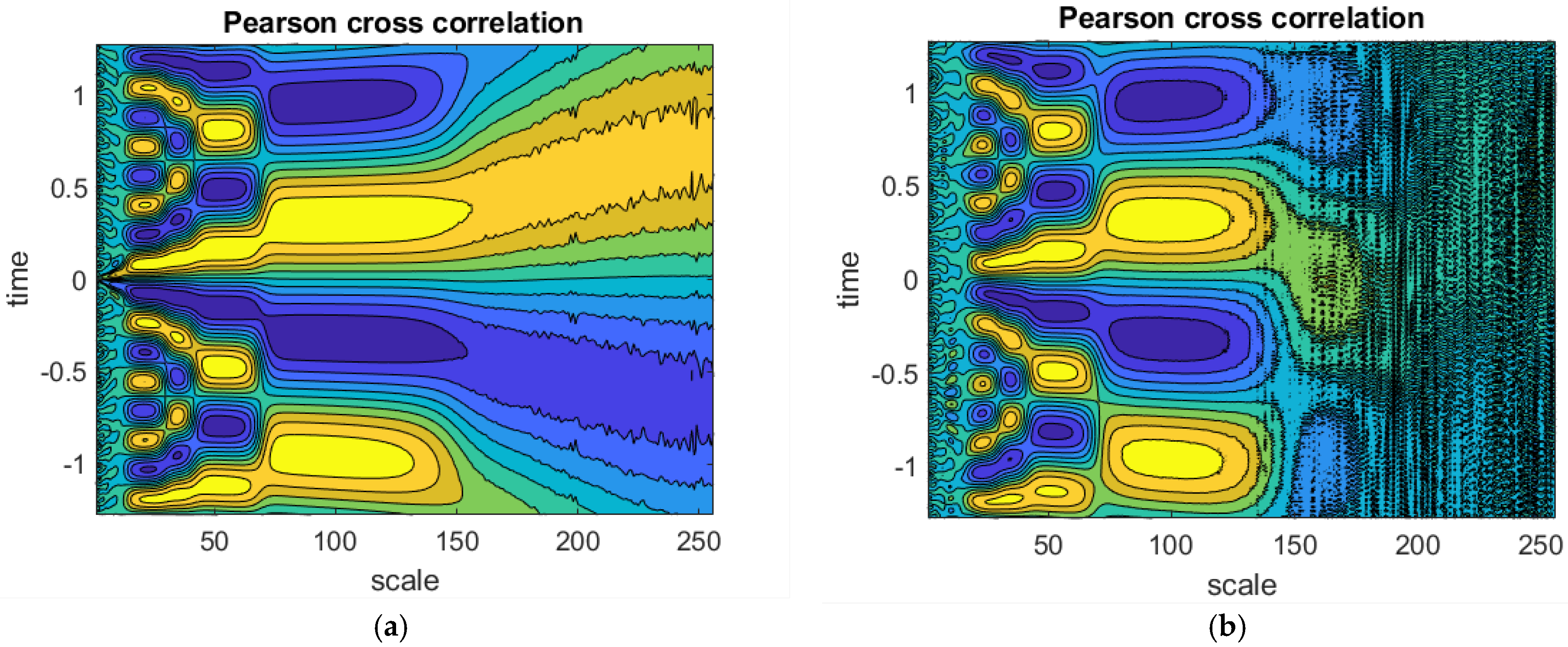
Two harmonic signals and , shifted relative to each other, were used to verify the results of the cross-wavelet correlation estimation, where , Gaussian white noise.
The results of estimating the cross-correlation coefficients are shown in Figure 3a,b. The time-shifted maxima of the cross-correlation of signals demonstrated the movement speed of inclusions of different sizes. The maxima of the correlation function reflect the velocities quite well. The correlation coefficients in Figure 3a were obtained for a signal-to-noise ratio SNR = 10, while in Figure 3b, the SNR was 1. A comparison of the results of the cross-correlation assessment showed that the presence of sufficiently powerful noise does not have a significant effect on determining the velocity of small inclusions.
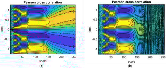
Figure 3.
Distribution of Pearson correlation coefficients by wavelet decomposition scales (a,b).
Non-orthogonal real Morlet wavelets are useful for processing signals that vary smoothly over time. The complex Morlet wavelet also allows one to analyze the phase characteristics of the harmonic components of the signal. Since oil well production streams contain some solids such as waxes and other impurities, RMT signals are not harmonic and contain non-additive Poisson noise, so orthogonal wavelets can be used. Orthogonal wavelet bases make it possible to obtain a compact and, perhaps, not smooth enough representation of signals.
2.4. Wavelet Cross-Correlation Based on Discrete Wavelet Transform
Orthogonal wavelets are characterized by two functions: a wavelet function and a scaling function. For their practical application of orthogonal and biorthogonal wavelets, fast transformation algorithms have been developed that use special filters. Feyer–Korovkin wavelets have good frequency localization and improved performance. These wavelets are more symmetrical but less smooth than the Daubechies wavelet. The frequency localization of Fejer–Korovkin filters guarantees a good representation of the signal in individual frequency bands. Even non-negative kernels generate quadrature mirror filters with optimal frequency localization [35].
The Fejer–Korovkin family combines compact, orthogonal wavelets used for both continuous and discrete transforms. The order of wavelets (4, 6, 8, 14, 18, or 22) must not exceed the logarithm of the number of data . The kernel of the Fejer–Korovkin filter has the form:
Each signal is represented as a linear combination of a scaling function and a wavelet at scales and offsets :
where is the number of wavelet decomposition levels.
The analysis of RMT signals was performed within a frame sliding along the signals, and we determined the undecimated wavelet transform. For signals , _frame, received in a frame of length , we determined the cross-correlation coefficients at each of the scales.
A total of coefficients and coefficients of details have been calculated. When decomposing a signal of length we can obtain no more than decomposition levels. Details are calculated at each level of decomposition, and coefficients are calculated only at the last level. For the data frame , the result is and the total number of levels, including the scale level .
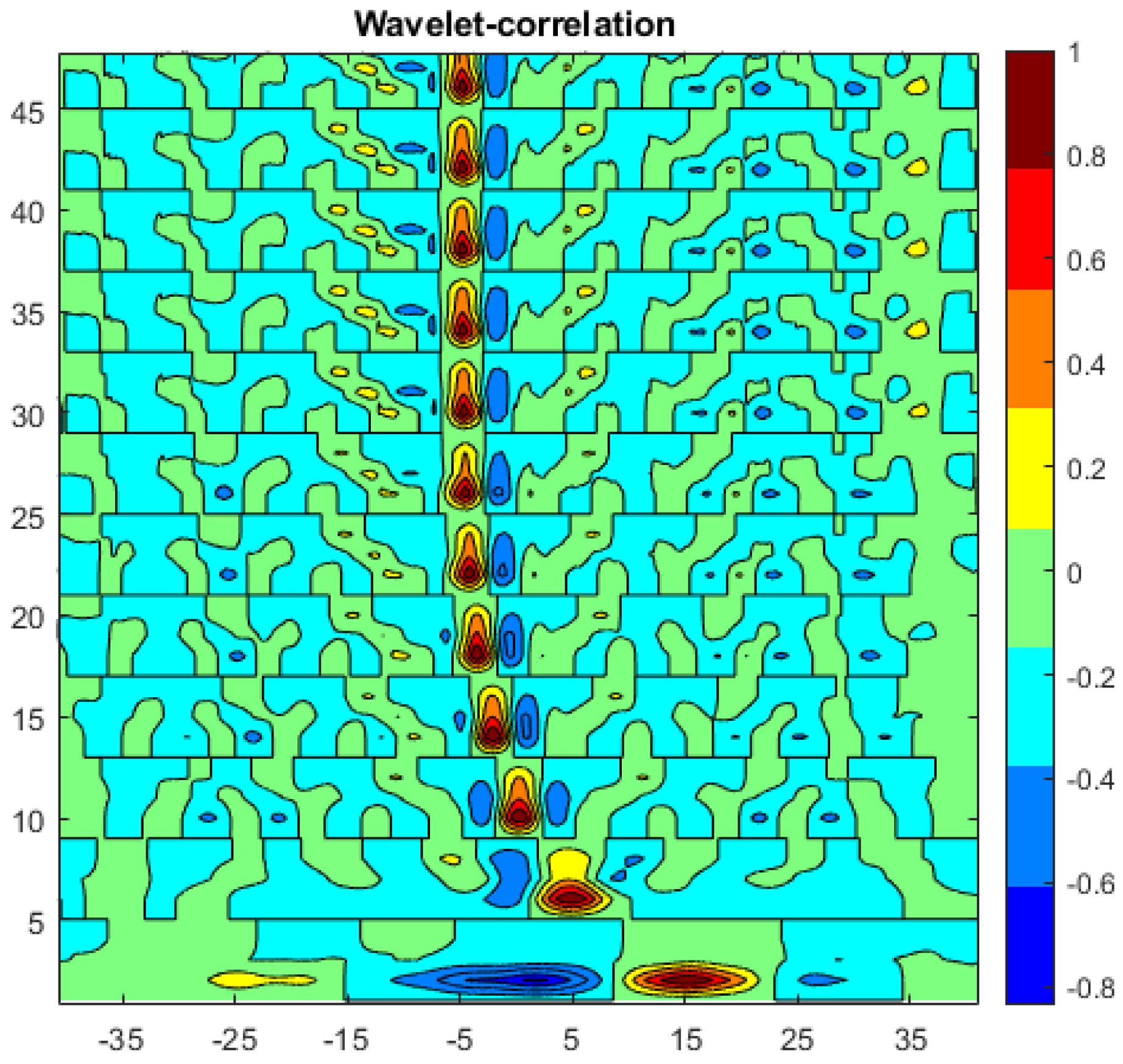
A computer experiment was conducted using a simplified model of the movement of a gas–oil mixture in a pipe with a dispersed bubble flow structure. The model for reducing the thickness of the oil layer that absorbs gamma rays in the presence of a bubble was determined by the formula Many bubbles were placed in the flow, the sizes of larger bubbles differed by their movement speeds were increased 1.5, 2.5, and 4 times. The simulation results are shown in Figure 4, which shows the displacement of the maximum of the correlation function in the wavelet decomposition spaces.
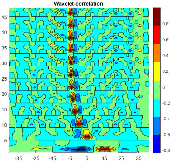
Figure 4.
Graphical representation of cross-correlation coefficients for 12 subspaces of the stationary non-decimated wavelet decomposition.
3. Results
3.1. Modeling of Gas–Liquid Flow
To test the method for measuring the speed of oil movement using the cross-correlation function in the spaces of wavelet decomposition of gamma density meter signals, a computer experiment was carried out using a simplified model of the movement of a gas–oil mixture in a pipe with a dispersed bubble flow structure [36]. Many authors pay attention to the modeling of multiphase flows, which are used in many production technologies [37,38,39,40]. In the petroleum industry, multiphase flow is highly relevant for predictive process design to ensure economical production and transportation of hydrocarbons. Modeling flow properties is of paramount importance for operating engineers, pump power calculations, and equipment control [41,42]. The intensity of the recorded gamma radiation is determined by the activity of the gamma radiation source, the density of the absorbing layer of liquid, its thickness, and linear attenuation coefficient, according to Bouguer’s law according to Equation (1).
Initially developed technological devices designed to monitor oil well production use an algorithm based on the autocorrelation function of the density RMT signal. When flow velocity is high, the autocorrelation function is narrow, and when the velocity decreases, it is wider. In the next version of systems, the autocorrelation function was replaced by a structure function, which does not require multiplication operations when calculated. This change made it possible to increase the speed of calculations performed in the technological devices. The next improvement to the system’s algorithm was the use of a derivative (finite difference) structure function, which emphasizes the high signal frequencies caused by the movement of small bubbles. With the increasing performance of industrial controllers, it has become possible to build an algorithm based on the wavelet transform presented in this article. The algorithm is more open; it allows analyzing the well flow structure and adjust the algorithm parameters to the most informative areas. The increased computational complexity of the proposed algorithm is compensated by faster calculations on a modern processor and the use of fast wavelet decomposition algorithms.
The intensity of radio emission from a Cs137 source is determined by the number of atoms of the radioactive element that decay per unit of time. During a series of experiments, the number of atoms decaying in each experiment changes. With the number of atoms that make up a sample of a radioactive element, is the probability with which the decay of any of the atoms of the sample is possible during the observation time. The number of photons produced during the decay of atoms is characterized by a random variable , which is characterized by the binomial law. The probability of registering photons in n trials is characterized by the probability:
where is the space of values of the random variable X, and is the number of combinations of n elements of elements.
The mathematical expectation of a binomial random variable is equal to the product of the number of trials and the probability of an event occurring in one trial: The variance of the binomial random variable X is equal to the product of the number of trials and the probability of the occurrence and non-occurrence of an event in one trial . Modeling probabilities using Equation (20) is not possible with large values of and low probability . If , then where is the parameter of Poisson’s law.
As increases, the Poisson distribution becomes more and more symmetric and turns into a Gaussian distribution. The Poisson distribution has the following characteristics: mathematical expectation , variance , standard deviation: , coefficient of skewness: , and coefficient of kurtosis: .
At a sufficiently high flux intensity, the number of detected photons has a Gaussian distribution, for which the mathematical expectation and variance are equal: , where is equal to the average number of atoms decaying per unit of time. The intensity of the recorded photon flux is the sum of the systematic and random components:
where is the average intensity of the emitted photon flux, in accordance with Equation (25), is the random noise component.
In the case of monoenergetic radiation with energy , radiation intensity is , where is the flux density at a certain point in space, i.e., related to the cross-sectional area. The scintillation detection unit is characterized by the effective registration area This value is determined for specific detector sizes by averaging the detection efficiency over their cross section. Calculation results for cylindrical detectors when registering with the side surface and the end surface direct radiation from the gamma source Cs-137 with energy , are presented in Table 1.

Table 1.
and values for cylindrical detectors.
With a known value of the number of pulses at the receiver output can be obtained from the expression:
Because the scintillation detection unit has a finite time resolution, to estimate the true count rate at the output of the scintillation detection unit, it is necessary to consider the number of pulses not registered by it (miscalculations).
3.2. Simulation Results
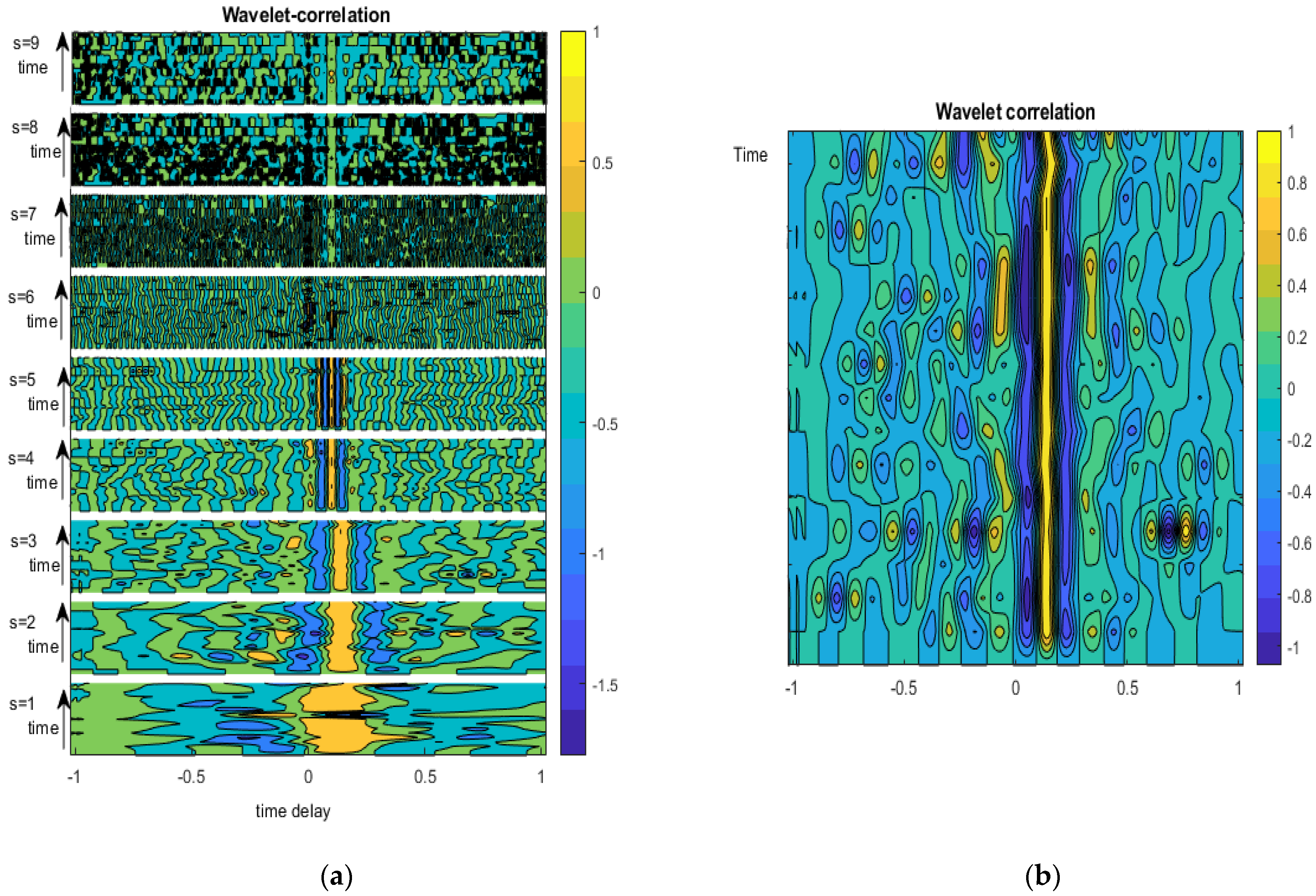
As a result of the simulation, the dependences of the cross-correlation of wavelet coefficients of two RMT signals on time on nine subspaces of decomposition were obtained. Figure 5a shows the time-varying cross-correlation of RMT signals at nine levels of wavelet decomposition. Since the movement speed of small bubbles corresponds to the speed of liquid, we find a suitable small scale and a corresponding maximum correlation in the figure. For this scale, using a graph, we determine the interval during which the oil flow passed the base distance. Based on the obtained distance, we derived the flow speed. Adding Poisson noise with signal-to-noise ratio , the cross-correlation estimate did not change significantly. Figure 5b shows the graph for the subspace , which best corresponds to the fluid motion.
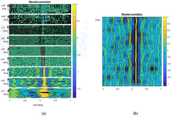
Figure 5.
Graphical representation of the time variation of cross-correlation coefficients for nine subspaces of the stationary non-decimated wavelet decomposition. (a) Representation in nine wavelet spaces; (b) representation in subspace 4.
In real conditions, the flows under study are not stationary, so the signal is analyzed within a sliding frame. The frame size must be chosen in such a way that it is possible to obtain the required number of wavelet decomposition levels.
Fluid speed is determined by the formula:
where is the distance between gamma radiation detectors, is the level of wavelet decomposition at which the movement of small bubbles is decisive.
Gas velocity depends on the movement of large bubbles and is determined in space at a lower level using the formula:
where is the level of wavelet decomposition at which the movement of large bubbles is decisive.
To determine the decomposition levels and , a neural network was used—a three-layer perceptron with a number of neurons, the input of which is the values , where the input layer takes decomposition space numbers ,, the inner layer has three neurons, the output layer generates signals and , and velocities .
The density of the oil and gas mixture is determined by the formula:
where is the number of gamma quanta obtained during the registration time when calibrating the system on an empty pipe, is the average number of gamma quanta obtained during the registration time during the measurement process, and is the number of gamma quanta received during the registration time at intervals classified as intervals of absence of free gas.
Classification of frames for recording and using a neural network to determine intervals of absence of free gas in the flow.
The density of the liquid is determined at intervals of absence of free gas:
The folume fraction of gas in the mixture:
where is the volume fraction of liquid in the mixture.
Volumetric gas flow—:
where is the cross-sectional area of the pipeline,
Volumetric fluid flow:
Mass gas flow :
Mass flow rate of the liquid phase of the flow:
A computer experiment using continuous Morlet wavelets and discrete Feyer–Korovkin wavelets and a simplified model of the movement of a gas–liquid mixture in a pipe with a dispersed bubble flow structure showed the possibility of simultaneous analysis of the structure of a two-phase flow and the speed of movement of gas inclusions. The assumption that the speed of movement of small gas inclusions corresponds to the speed of the liquid allows us to determine the speed of the liquid part of the flow. To more accurately account for the relationship between the speed of fluid movement, instrument calibration is used. Calibration tests also make it possible to consider the stochastic nature of the intensity of radioisotope radiation, which is related to the coefficient of linear attenuation of radiation, the density and thickness of the absorbing layer according to Bouguer’s law, shown by Equation (1). During the modeling process, Poisson noise was taken into account, the variance of which is equal in value to the mathematical expectation of the signal The average signal-to-noise ratio is approximately , where is the standard deviation of the signal and noise, respectively. When calculating the fluid speed, a frame of 4096 samples was used. Frame was shifted along the signal sample by 2046 samples. This shift corresponds to the rectangular window.
The instrument was calibrated using a specially designed calibration installation. For grading, it was enough to use a small neural network—a three-layer perceptron with the number of neurons 3-3-1 and with the “Hyperbolic tangent” , is the induced local field of the neuron, for the first and second layers and a linear activation function at the output.
4. Discussion
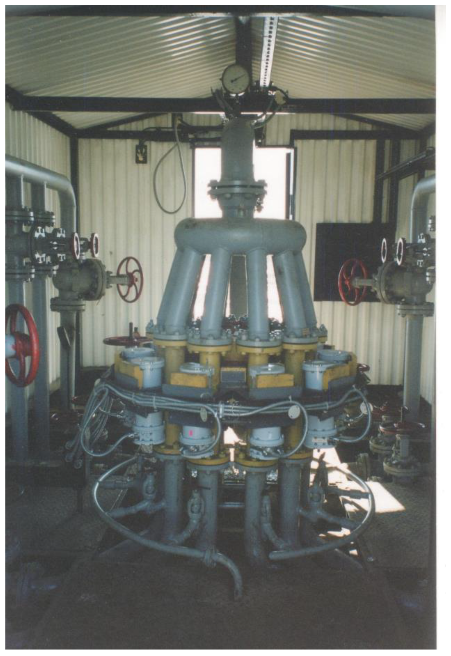
The proposed algorithm for processing the signal of a photon density meter of a two-phase flow of oil well production makes it possible to monitor oil production processes for any flow structure, characteristic of both fields with difficult-to-recover heavy paraffinic, resinous oil, and fields with simpler flows. Wavelet cross-correlation, presented in the form of an image, characterizes the instantaneous structure of the flow, and the sequence of such images characterizes the dynamics of the flow of a complex structure. The proposed control method works with flows of any structure that have different ratios between phase flow rates, and therefore is universal. Its versatility allows you to control the production processes for the entire well stock. Figure 6 shows the appearance of a device that controls the production processes of a group of wells.
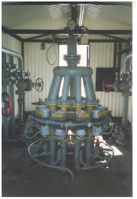
Figure 6.
Design of a multi-channel device that performs measurements for an entire cluster of wells.
The number of input layer nodes is determined by the number of wavelet decomposition levels: . The first hidden layer of the MLP has eight fully connected neurons with an activation function:
where is the output signal of the neuron adder, characterizing its local field, and is a mathematical constant. The output layer contains two neurons that generate signals for the speed of liquid and gas .
MLP training was performed using the Levenberg–Marquard method of backpropagation of errors over time in real time. Two types of data are used to train a neural network. The first type of data is obtained by simulating the passage of gamma rays through matter.
The advantages of using a radioisotope converter and the wavelet decomposition method of its signal are mainly the following:
- –
- Elimination of the process of preliminary separation of a multiphase flow with the release of the liquid component.
- –
- Lack of hydraulic resistance to oil flow.
- –
- No restrictions on viscosity or chemical activity of the controlled flow.
- –
- Insensitive to deposits on the inner surface of the pipe.
- –
- The ability to create a multi-channel device that performs measurements for an entire cluster of wells.
Non-contact allows for measurement and control in aggressive environments. During the day, the flow rate can change by tens of a percent. Periodic testing does not allow you to see the dynamics of well productivity in real time, diagnose the technical condition of equipment, and predict the technological process. The advantage of the proposed method is the continuity of measurement and control of the oil and gas production process throughout the entire field.
5. Conclusions
To improve the efficiency of oil production process control, it is advisable to use separation-free non-contact measurement of multiphase product flows from oil wells. The physical basis of control is radioisotope measuring transducers, which provide a signal containing information about the structure of the two-phase flow, the speed of movement of liquid and gas, and the relative content of gas and liquids in the general flow. The measurement algorithms closest to our study use autocorrelation, structural, or cross-correlation functions, which do not allow the structure of two-phase flow to be considered. An algorithm based on cross-correlation of CWT coefficients allows obtaining more information to control production processes. The flow rates of liquid and gas are determined by the marking method, with bubbles of free gas in the liquid being used as natural flow marks. Tag velocities are measured using the cross-correlation method.
The proposed method is based on calculating the cross-correlation of wavelet coefficients in expansion spaces, the number of which depends on the structure of the two-phase flow. In this case, it is appropriate to use Pearson cross-correlation, which is applied in real time to the signal frame, shifted with an overlap depending on the type of window selected. For measurement purposes, either continuous wavelet transforms or discrete wavelet transforms can be used, for which cross-correlation can be calculated for both the approximation coefficients and the detail coefficients. In the latter case, the maximum will be sharper. The discrete wavelet transform has fast decomposition-reconstruction algorithms and is therefore preferred. The continuous wavelet transforms using Morlet wavelets, which is a harmonic function with a Gaussian window, is slower. To suppress noise, it is advisable to perform smoothing in time and space of the wavelet decomposition.
The correlation between wavelet decomposition spaces allows smoothing to be performed and better identify the spaces containing useful information. Training a neural network at the stage of calibration of the measuring installation makes it possible to adapt the algorithm, determine the subspaces of the wavelet decomposition containing information about the flow structure, and determine the speed, density, and flow rate of oil well production. It is advisable to adapt the algorithm using a neural network for each well that has its own different type of flow.
With continuous measurement, we are dealing with data frames of finite length, therefore, when performing CWT, errors at the ends of the frames will be the same as during the Fourier transform, because both methods assume that the data is cyclical. Before performing the wavelet transform, it is recommended to pad the frames with zeros. With cyclic conversion, there is no need to pad frames with zeros, and there are no errors at the edges.
It seems promising to use the wavelet decomposition algorithm and a convolutional neural network to automatically analyze the wavelet decomposition image and determine from it the structure of the product flow and the productivity of an oil well.
6. Patents
Zarur L., Malykhina G.F. Intelligent System and Method for Measuring the Flow of Two-Phase Flow of Oil Wells. Patent for invention RU 2,793,366 C1, 31 March 2023. Application No. 2021137385 dated 16 December 2021.
Author Contributions
Conceptualization, D.K. and G.M.; methodology, D.A.; software, G.M.; validation, D.A., G.M. and D.K.; formal analysis, D.A.; investigation, G.M.; resources, D.K.; data curation, D.K.; writing—original draft preparation, G.M.; writing—review and editing, D.A.; visualization, D.K.; supervision, G.M.; project administration, D.A.; funding acquisition, G.M. All authors have read and agreed to the published version of the manuscript.
Funding
This research was funded by the Ministry of Science and Higher Education of the Russian Federation as part of the World-class Research Center program: Advanced Digital Technologies grant number 075-15-2022-311 dated 20 April 2022.
Data Availability Statement
Acknowledgments
The authors thank the scientific supervisors of the project who provided the necessary equipment and the laboratory staff for constructive discussion of the research results.
Conflicts of Interest
Author Dmitry Kratirov was employed by the company LLC “Complex-Resource”. The remaining authors declare that the research was conducted in the absence of any commercial or financial relationships that could be construed as a potential conflict of interest. The LLC “Complex-Resource” had no role in the design of the study; in the collection, analyses, or interpretation of data; in the writing of the manuscript, or in the decision to publish the results.
References
- Fazlyyakhmatov, M.G.; Sabitov, L.S.; Lazarev, D.K. Methods and Means of Measuring the Amount of Oil and Gas: Textbook. Allowance; Kazan University Publishing House: Kazan, Russia, 2021; 256p. (In Russian) [Google Scholar]
- Meribout, M.; Azzi, A.; Ghendour, N.; Kharoua, N.; Khezzar, L.; AlHosani, E. Multiphase Flow Meters Targeting Oil & Gas Industries. Measurement 2020, 165, 108111. [Google Scholar]
- Kozelkova, V.; Kozelkov, O.; Dudkin, V. Online Multiphase Flow Measurement of Crude Oil Properties Using Nuclear (Proton) Magnetic Resonance Automated Measurement Complex for Energy Safety at Smart Oil Deposits. Energies 2023, 16, 1080. [Google Scholar] [CrossRef]
- Ramakrishnan, V.; Arsalan, M. A Pressure-Based Multiphase Flowmeter: Proof of Concept. Sensors 2023, 23, 7267. [Google Scholar] [CrossRef] [PubMed]
- Ünalmis, Ö.H. A Methodology for In-Well Multiphase Flow Measurement with Strategically Positioned Local and/or Distributed Acoustic Sensors. Sensors 2023, 23, 5969. [Google Scholar] [CrossRef] [PubMed]
- Muzipov, K.N. Theory and Practice of Flowmetry of Oil Wells Multiphase Production UDC. Autom. Informatiz. Fluel Energy Complex 2021, 3, 5–10. (In Russian) [Google Scholar]
- Zemenkov, Y.D.; Zaitsev, E.V.; Shabarov, A.B. Measurement of phase flow in water, oil and gas media using infrared radiation. In IOP Conference Series: Materials Science and Engineering; IOP Publishing: Bristol, UK, 2019; Volume 663, p. 012002. [Google Scholar]
- Wang, M.; Song, H.; Shi, X.; Liu, W.; Wei, B.; Wei, L. Dynamic Monitoring of Low-Yielding Gas Wells by Combining Ultrasonic Sensor and HGWO-SVR Algorithm. Processes 2023, 11, 3177. [Google Scholar] [CrossRef]
- Masoumeh, Z.; Michael, J.L.; Aljindan, L.; Noui-Mehidi, J.M.; Nabil, M.; O’Neill, K.T. Nuclear Magnetic Resonance Multiphase Flowmeters: Current Status and Future Prospects. SPE Prod. Oper. 2021, 36, 423–436. [Google Scholar]
- Kornienkoa, V.; Avtonomova, P. Application of Neutron Activation Analysis for Heavy Oil Production Control. Procedia-Soc. Behav. Sci. 2015, 195, 2451–2456 . [Google Scholar] [CrossRef]
- Roshani, M.; Phan, G.T.; Ali, P.J.M.; Roshani, G.H.; Hanus, R.; Duong, T.; Corniani, E.; Nazemi, E.; Kalmoun, E.M. Evaluation of flow pattern recognition and void fraction measurement in two phase flow independent of oil pipeline’s scale layer thickness. Alex. Eng. J. 2021, 60, 1955–1966. [Google Scholar] [CrossRef]
- Roshani, G.H.; Ali, P.J.M.; Mohammed, S.; Hanus, R.; Abdulkareem, L.; Alanezi, A.A.; Sattari, M.A.; Amiri, S.; Nazemi, E.; Eftekhari-Zadeh, E.; et al. Simulation Study of Utilizing X-ray Tube in Monitoring Systems of Liquid Petroleum Products. Processes 2021, 9, 828. [Google Scholar] [CrossRef]
- Nazemi, E.; Feghhi, S.A.H.; Roshani, G.H.; Setayeshi, S.; Peyvandi, R.G. A radiation-based hydrocarbon two-phase flow meter for estimating of phase fraction independent of liquid phase density in stratified regime. Flow Meas. Instrum. 2015, 46 Pt A, 25–32. [Google Scholar] [CrossRef]
- Denislamov, I.Z.; Shadrina, P.N.; Portnov, A.Y. Quantitative diagnostics methods for asphalt-region paraffin deposits in wells and oil pipelines. Dev. Oper. Oil Gas Fields 2019, 2. [Google Scholar]
- Nguyen, V.T.; Pham, T.V.; Rogachev, M.K.; Korobov, G.Y.; Parfenov, D.V.; Zhurkevich, A.O.; Islamov, S.R. A comprehensive method for determining the dewaxing interval period in gas lift wells. J. Petrol. Explor. Prod. Technol. 2023, 1, 1163–1179. (In Russian) [Google Scholar]
- Povyshev, K.I.; Vershinin, S.A.; Vernikovskaya, O.S. Oil and gas condensate fields. A systematic approach to multiphase flow control. Prof. Oil 2017, 4, 59–63. [Google Scholar]
- Poelma, C. Measurement in opaque flows: A review of measurement techniques for dispersed multiphase flows. Acta Mech. 2020, 231, 2089–2111. [Google Scholar] [CrossRef] [PubMed]
- Li, D.-H.; Wu, Y.-X.; Li, Z.-B.; Zhong, X.-F. Volumetric fraction measurement in oil-water-gas multiphase flow with dual energy gamma-ray system. J. Zhejiang Univ. Sci. A 2005, 6, 1405–1411. [Google Scholar]
- Taylan, O.; Abusurrah, M.; Amiri, S.; Nazemi, E.; Eftekhari-Zadeh, E.; Roshani, G.H. Proposing an Intelligent Dual-Energy Radiation-Based System for Metering Scale Layer Thickness in Oil Pipelines Containing an Annular Regime of Three-Phase Flow. Mathematics 2021, 9, 2391. [Google Scholar] [CrossRef]
- Baek, M.K.; Chung, Y.S.; Lee, S.; Kang, I.; Ahn, J.J.; Chung, Y.H. Design of a Nuclear Monitoring System Based on a Multi-Sensor Network and Artificial Intelligence Algorithm. Sustainability 2023, 15, 5915. [Google Scholar] [CrossRef]
- Khamehchi, E.; Zolfagharroshan, M.; Mahdiani, M.R. A robust method for estimating the two-phase flow rate of oil and gas using wellhead data. J. Petrol. Explor. Prod. Technol. 2020, 10, 2335–2347. [Google Scholar] [CrossRef]
- Malykhina, G.F.; Zarour, L.; Tarkhov, D.A. Measurement of the Volume of Gaseous and Liquid Fraction of the Flow of Oil Wells. In Proceedings of the International Multi-Conference on Industrial Engineering and Modern Technologies (FarEastCon), Vladivostok, Russia, 6–9 October 2020; IEEE: Piscataway, NJ, USA, 2020; pp. 1–5. [Google Scholar] [CrossRef]
- Martynov, D.R. Structure of upsending two-phase gas-liquid flow in the mode of natural circulation in an inclined channel under conditions of significant influence of mass forces. Polytech. Youth Mag. 2018, 9. (In Russian) [Google Scholar] [CrossRef]
- Zilges, A.; Babilon, M.; Hartmann, T.; Savran, D.; Volz, S. Collective excitations close to the particle threshold. Prog. Part. Nucl. Phys. 2005, 55, 408–416. [Google Scholar] [CrossRef]
- Androsenko, P.A.; Popova, G.V. An efficient method of modelling the klein-nishina-tamm distribution. USSR Comput. Math. Math. Phys. 1981, 21, 4. [Google Scholar] [CrossRef]
- Tsakiroglou, C.D.; Sygouni, V.; Aggelopoulos, C.A. Aggelopoulos, Using multi-level wavelets to correlate the two-phase flow characteristics of porous media with heterogeneity. Chem. Eng. Sci. 2010, 65, 6452–6460. [Google Scholar] [CrossRef]
- Rinoshika, A.; Rinoshika, H. Application of multi-dimensional wavelet transform to fluid mechanics. Theor. Appl. Mech. Lett. 2020, 10, 98–115. [Google Scholar] [CrossRef]
- Munir, M.W.; Khalil, B.A. Cross correlation velocity measurement of multiphase flow. Int. J. Sci. Res. 2015, 4, 802–807. [Google Scholar]
- Yan, H.; Zhang, Y.; Yang, Q. Time-Delay Estimation Based on Cross-Correlation and Wavelet Denoising. In Proceedings of 2013 Chinese Intelligent Automation Conference. Lecture Notes in Electrical Engineering; Sun, Z., Deng, Z., Eds.; Springer: Berlin/Heidelberg, Germany, 2013; Volume 255. [Google Scholar]
- Zhao, B.; Ju, B.; Wang, C. Initial-Productivity Prediction Method of Oil Wells for Low-Permeability Reservoirs Based on PSO-ELM Algorithm. Energies 2023, 16, 4489. [Google Scholar] [CrossRef]
- El-Hashash, E.F. Comparison of the Pearson, Spearman Rank and Kendall Tau Correlation Coefficients Using Quantitative Variables. Asian J. Probab. Stat. 2022, 20, 36–48. [Google Scholar] [CrossRef]
- Bozhokin, C.V.; Zharko, S.V.; Larionov, N.V.; Litvinov, A.N.; Sokolov, I.M. Wavelet correlation of non-stationary signals. J. Tech. Phys. 2017, 87, 822–830. (In Russian) [Google Scholar]
- Bravo, S.; González-Chang, M.; Dec, D.; Valle, S.; Wendroth, O.; Zúñiga, F.; Dörner, J. Using wavelet analyses to identify temporal coherence in soil physical properties in a volcanic ash-derived soil. Agric. For. Meteorol. 2020, 285–286, 107909. [Google Scholar]
- Sharkova, S.B.; Faerman, V.A. Wavelet transform-based cross-correlation in the time-delay estimation applications. J. Phys. Conf. Ser. 2021, 2142, 012019. [Google Scholar] [CrossRef]
- Solomon, I.; Kumar, U. Fast Wavelet Transform. In Encyclopedia of Mathematical Geosciences; Daya Sagar, B.S., Cheng, Q., McKinley, J., Agterberg, F., Eds.; Encyclopedia of Earth Sciences Series; Springer: Cham, Switzerland, 2023. [Google Scholar]
- Zhu, X.; Haglind, F. Computational fluid dynamics modeling of liquid–gas flow patterns and hydraulics in the cross-corrugated channel of a plate heat exchanger. Int. J. Multiph. Flow 2020, 122, 103163. [Google Scholar] [CrossRef]
- Pei, Y.; Zhang, N.; Zhou, H.; Zhang, S.; Zhang, W.; Zhang, J. Simulation of multiphase flow pattern, effective distance and filling ratio in hydraulic fracture. J. Petrol. Explor. Prod. Technol. 2020, 10, 933–942. [Google Scholar] [CrossRef]
- Shynybayeva, A.; Rojas-Solórzano, L.R. Eulerian–Eulerian Modeling of Multiphase Flow in Horizontal Annuli: Current Limitations and Challenges. Processes 2020, 8, 1426. [Google Scholar] [CrossRef]
- Olafadehan, O.A.; Abhulimen, K.E.; Anubi, M. Grid design and numerical modeling of multiphase flow in complex reservoirs using orthogonal collocation schemes. Appl. Petrochem. Res. 2018, 8, 281–298. [Google Scholar] [CrossRef]
- Nguyen, V.-T.; Phan, T.-H.; Duy, T.-N.; Kim, D.-H.; Park, W.-G. Fully compressible multiphase model for computation of compressible fluid flows with large density ratio and the presence of shock waves. Comput. Fluids 2022, 237, 105325. [Google Scholar] [CrossRef]
- Jordanou, J.P.; Camponogara, E.; Antonelo, E.A.; Schmitz, M.A. Nonlinear Model Predictive Control of an Oil Well with Echo State Networks. IFAC 2018, 51, 13–18. [Google Scholar] [CrossRef]
- Adukwu, O.; Odloak, D.; Kassab, F., Jr. Optimisation of a Gas-Lifted System with Nonlinear Model Predictive Control. Energies 2023, 16, 3082. [Google Scholar] [CrossRef]

Disclaimer/Publisher’s Note: The statements, opinions and data contained in all publications are solely those of the individual author(s) and contributor(s) and not of MDPI and/or the editor(s). MDPI and/or the editor(s) disclaim responsibility for any injury to people or property resulting from any ideas, methods, instructions or products referred to in the content. |
© 2024 by the authors. Licensee MDPI, Basel, Switzerland. This article is an open access article distributed under the terms and conditions of the Creative Commons Attribution (CC BY) license (https://creativecommons.org/licenses/by/4.0/).