Abstract
A zone control algorithm is proposed that considers both economic performance indicators and control performance indicators. Unlike classic set point control, zone control expands the control target into a convex set. In this study, an ellipsoid is used as the control target, and the advantages of the ellipsoid target are explained in terms of overall stability and computational load. After defining the distance measurement function and appropriate terminal constraints, an objective function that considers both control performance and optimization performance is constructed. A theoretical analysis shows that the proposed control algorithm satisfies the Lyapunov stability criterion. The superiority of the ellipsoid control target in handling complex multivariable control tasks is also demonstrated. This method has significant potential value in practical industrial applications, helping to unleash the potential control performance and economic benefits of zone control systems. Finally, the feasibility and stability of the algorithm are verified through a typical chemical process simulation.
1. Introduction
In process control, the system usually has complex features such as multivariable, strong coupling, large dead time and nonlinearity. These complex features bring difficulties to the design of classic controllers. Therefore, many modern control theories have been established to overcome the complex characteristics of the system. Model predictive control (MPC), as a model-based multi-variable control algorithm, has been widely studied and applied [1,2,3,4]. In the MPC algorithm, the physical constraints of the system are used as the corresponding hard constraints of the controller, and the control objective of the system is reflected by the objective function, which is the soft constraint. By continuously solving the optimization problem at each time, the best control law at each sampling time can be obtained. Due to the limitation of computers’ computing power, the early MPC could only satisfy a simple paradigm. With the development of computer hardware and software, great progress has been made in the field of linear programming and non-linear programming, and corresponding solutions for complex optimization problems have been provided. Therefore, MPC control algorithms suitable for various scenarios can be developed. In industrial applications, MPC control strategies have been used to cope with various complex multi-variable systems. At the same time, the MPC control strategy is also developing towards high flexibility. In the theoretical part, researchers have proposed a variety of design paradigms based on the Lyapunov stability criterion.
The realization of an MPC controller depends on solving optimization problems with constraints. These optimization problems use the observations of the system state variables at the current sampling time to predict the state trajectory in the future finite horizon, and they output the first element of the optimal control sequence under a given optimization goal. At the next sampling time, the above solution process is repeated to obtain a new optimal control law. Rawlings and Muske [5] developed an infinite horizon predictive control that includes input and state constraints. Research shows that state constraints can be removed under certain conditions, and the solution of the optimization problem can be obtained by finite-dimensional quadratic programming. Grimm et al. [6] developed a finite horizon MPC controller for unconstrained nonlinear systems and proved that the closed-loop system is still stable without terminal constraints. Primbs and Nevistić [7] discussed the relationship between the prediction horizon and the stability of the closed-loop system. For compact initial conditions, there is a prediction horizon such that any horizon greater than this value can satisfy stability. Lee et al. [8] developed a constrained nonlinear predictive controller. The algorithm includes terminal constraints and relies on an online linear programming problem. At the same time, it is pointed out that suitable terminal constraints can ensure the asymptotic stability.
With the development of MPC technology, its application scenarios have become more diverse. Since the MPC control strategy is based on a mathematical model, a model with a complex mathematical form [9] or a model with a complex operating rule [10] can obtain better simulation results under the MPC framework. There are many ways to obtain the reference model in MPC. Wibowo and Saad [11] analyzed and compared multiple identification methods and designed an identification strategy. The identification model can reproduce the main dynamic characteristics of the real system. Similarly, the data-driven MPC strategy [12] and the MPC controller based on encrypted Lyapunov technology [13] have been successfully applied. Dubay [14] developed a self-optimized MPC controller for the highly nonlinear injection moulding process to ensure product quality. Oravec et al. [15] developed a robust MPC control strategy with soft constraints for the nonlinear process with asymmetric dynamic characteristics and improved the performance of the system in the response process through soft constraints. In the building temperature control system, awryńczuk and Ocłoń [16] used a double-layer structure of an optimizer and MPC controller. The optimizer can calculate the optimal operating point online to minimize energy consumption. The simulation results show the effectiveness of this strategy. In addition, Zhao and Go [17] developed a two-layer MPC control strategy. The collision avoidance reference trajectory is calculated by the upper MPC controller, and the trajectory tracking is realized by the robust feedback controller. Similarly, the distributed MPC strategy developed by Dai et al. [18] also implements functions such as collision avoidance and obstacle avoidance for multiple agents. Rahman et al. [19] achieved precise control of the blow-line Kappa number by feedforwarding lignin content measurements using near-infrared spectroscopy and MPC controller. Zhao et al. [20] used fractional order MPC technology to achieve improved control performance of the steam/water loop. He et al. [21] employed MPC technology to achieve optimized tool paths for forming parts with varying wall angles in incremental sheet forming.
Based on MPC, researchers have developed economic model predictive control (EMPC) that can directly use economic index functions as objective functions. This control strategy has been fully developed in theory and application as MPC strategy [22]. In fact, the implementation paradigm of EMPC is similar to that of MPC, but there are differences between the two control strategies for the proof of stability. Adeodu et al. [23] developed an infinite horizon EMPC controller, which represented the objective function of the infinite horizon by an approximate term, and verified the effectiveness of the strategy through simulation experiments. Liu and Liu [24] discussed the impact of the finite horizon in the terminal loss function on the performance of the closed-loop system. Grüne [25] considered an EMPC control strategy without terminal constraints and gave an upper bound for the loss of this strategy. Similarly, based on MPC, integrating economic optimization factors in its solution process can still construct a control strategy with economic optimization behavior [26,27]. In addition, there are control performances corresponding to economic performance indicators, such as the form of control targets. When the control target expands from a set point to a convex set, the problem can be summarized as zone control. González and Odloak [28] developed a zone MPC control strategy, which can ensure that the closed-loop stability is satisfied both inside and outside the zone control target. Graciano et al. [29], Capron and Odloak [30] used multi-layer MPC, where the top layer is an optimizer, and the bottom layer is a zone MPC controller. The optimizer can calculate the optimal operating point, and the MPC controller can move the system to the preset operating point under constraint conditions. Ferramosca et al. [31] developed a zone tracking MPC control strategy, using a distance metric to ensure recursive feasibility and local optimality, and verified the performance of the proposed strategy through simulation experiments. Guan et al. [32] developed a zone control algorithm based on soft constraints to reduce the frequency of zone constraint violations and increase the stability of the closed-loop system. It is worth mentioning that under the framework of zone control, the system still has additional degrees of freedom after entering the zone target. According to this degree of freedom, an optimization strategy can be designed to improve the economic benefits of the zone control system [33].
The main contributions of this paper are as follows:
- Propose a zone predictive control algorithm for ellipsoid control targets.
- Analyze typical switching control strategies and geometric forms in multi-stage control systems.
- Theoretically analyze the finite-time occurrence of switching in switching strategies.
- Verify the effectiveness of the control strategy through numerical simulations.
In this paper, a typical switching control strategy is introduced in a multi-stage control system. The differences between the geometric forms of the zone control targets are then explained. Subsequently, a control algorithm corresponding to the ellipsoid control target is designed, and the stability of the closed-loop system is theoretically ensured. Common problems in multi-stage control are discussed sequentially from Section 2, and reasonable solutions are provided. The geometric form of the control target is analyzed, leading to the selection of the ellipsoid control target as being more suitable for this strategy. In Section 3, a zone predictive control algorithm is developed, and the stability of its closed-loop system is analyzed. Section 4 presents numerical simulation experiments used to verify the effectiveness of the proposed control strategy.
2. Motivation
2.1. The Two Stages Control Strategy
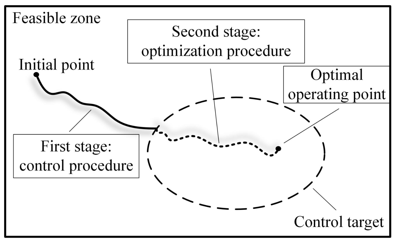
In zone control, the trajectory of the system state can be divided into two stages, as shown in Figure 1. In the first stage, the system state is outside the control target. At this stage, the controller should the take control performance as the main factor and weaken optimization operations such as economic optimization or quality optimization. In the second stage, the system state is inside the control target, and optimization operations such as economic optimization should be considered at this time. In addition, the controller of the second stage needs to ensure the asymptotic stability of the closed-loop system and prevent the system state from deviating from the control target due to optimized operation. In other words, the controller needs to ensure the convergence of the zone control targets during the optimization stage. Therefore, zone control can be regarded as a multi-objective control problem, and its control objective in the first stage is a set of points. The switching points of these two stages are strictly defined in some scenarios. For example, in process control, when the system state enters the zone control target, it can be considered that the first stage of the control process has ended. The next step is to start the economic optimization operation, which is to start the second stage to improve the economic performance of the entire closed-loop system. From the perspective of actual production, when the product has not yet reached the quality score that meets the customer’s requirements, there is no need to consider improving economic efficiency during the production. It is meaningful to consider the economic optimization in the production process only when the various indicators of the product meet the requirements. Therefore, the two-stage control strategy is more reasonable in process control.

Figure 1.
The schematic of two stages of zone control.
From the point of view of control theory, there are two possible reasons that explain why the system does not need to perform economic optimization when the system state is outside the control target.
Within the framework of EMPC or optimal control, the optimal trajectory depends on the mathematical model of the system. Usually, the controller designer chooses the local linearized model near the steady-state operating point as the reference model. This model can show the characteristics of the system within a given accuracy error near the steady-state point. Once the operating range is not within this neighborhood, accuracy errors cannot be guaranteed. Therefore, there is a varying model accuracy error between the current state of the system and the steady-state operating point, and the model error becomes larger as the distance increases, as shown in Figure 2.
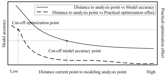
Figure 2.
The schematic of optimization effect and model accuracy vs. distance to operating point.
Consider a discrete system as follows:
Assume that the steady-state point satisfies . Define = as the model error of the linear model; then, the linearization model at the steady-state point is shown in Equation (2).
where , .
Assumption 1.
Linearization model error , where the monotonically increasing and zero-starting -class function is strictly increasing and satisfies .
Lemma 1.
For any , there exists an ellipsoid , so that for , the linearized system of satisfies .
Proof.
According to assumption 1, . Select ; let ; then, is established. So, for , both and are established. □
From Remark 1, the necessity of multi-stage control can be derived. That is, the model error within the specified range can meet the given requirements.
Therefore, in practical applications, the control target or the cut-off optimization point must be determined by the characteristics of the process and operating conditions, including safety, availability, reliability, accuracy, weight, and size.
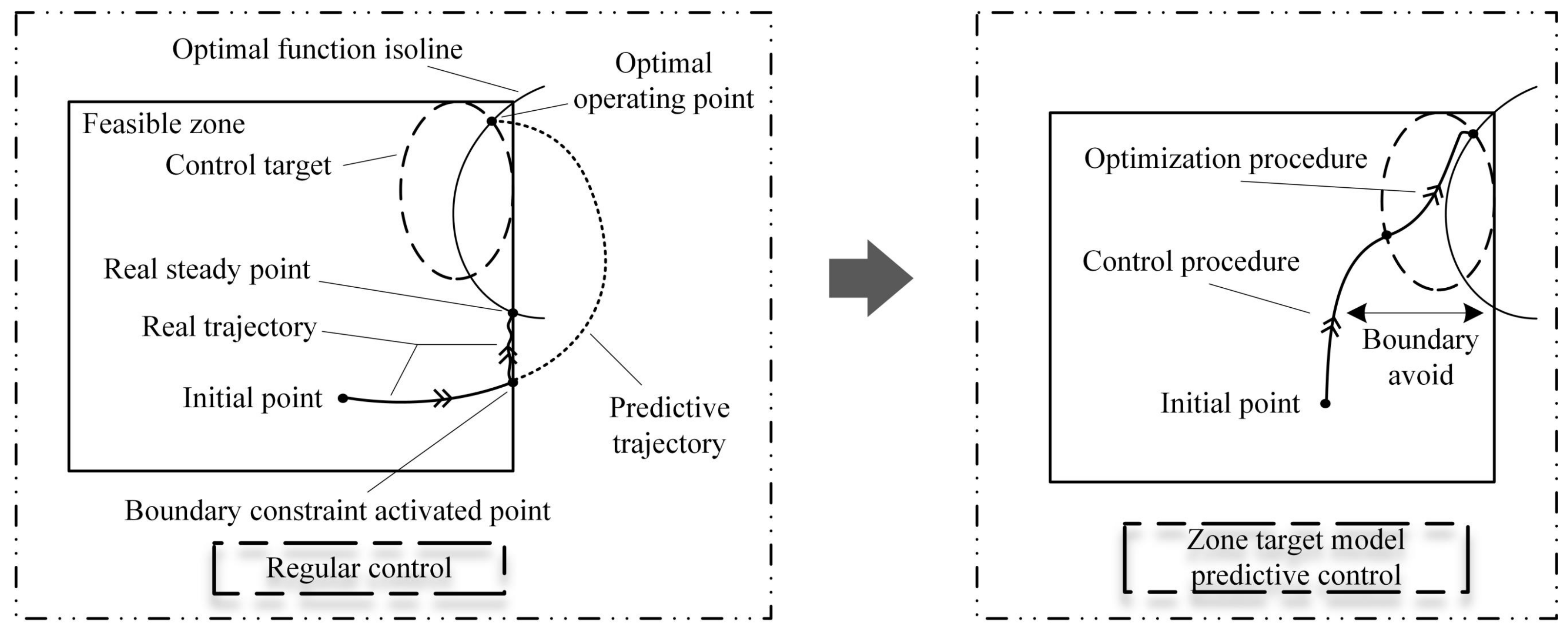
On the other hand, the control strategy of optimizing and controlling separation can reduce the risk of failure in the optimization process. Conventional control may result in the optimization operation not being as expected, as shown in the left half of Figure 3. The controller drive system advances along the predicted optimal trajectory, and the system’s feasible domain limiting factors prevent the system from advancing along the set trajectory. Finally, the system is limited to the same contour as the best working point, but it does not enter the setting zone. From the experimental phenomenon, the system is locked at the boundary of the feasible domain, resulting in a boundary effect. Therefore, the control strategy should be designed to avoid boundary effects.

Figure 3.
The schematic of regular control vs. zone target model predictive control.
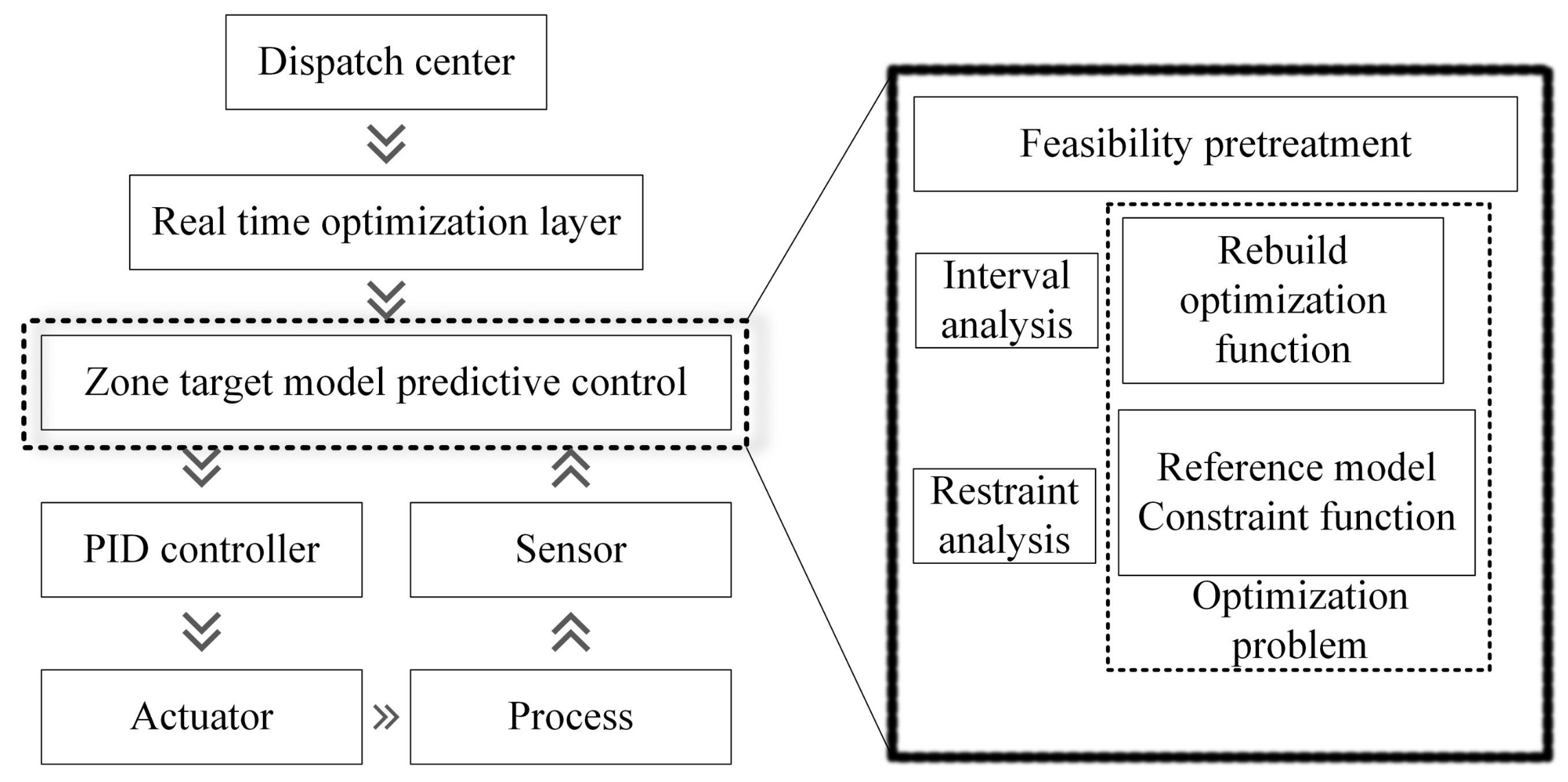
In the design of the control strategy, additional parts should be added to avoid boundary effects, as shown in Figure 4. Feasible domain preprocessing is performed at the beginning of the algorithm, while two asynchronous monitoring events are designed to analyze the behavior of the system online. Within this framework, there are two independent processing strategies that ensure that the system can optimally control the system during the control process and optimization process. In a two-stage control strategy, boundary effects can be effectively avoided. The trajectory of the system under this control strategy can be referred to on the right half of Figure 3. The state of the system is driven to the set zone first and then gradually stabilized to the optimal operating point.

Figure 4.
The framework of the zone control system.
2.2. The Ellipsoid Control Target
In this section, the spatial geometry of the zone control target is the focus. This problem is analyzed from two different perspectives: algorithm complexity and control performance. First, let us take the cube and ellipsoid in space as examples to find out the computer resources that the algorithm needs to consume in these two cases. When the controller needs to determine the distance between the current state and the set target, a spatial search algorithm is initiated to obtain a more accurate distance. In the spatial cube control target, the n-dimensional setting target divides the space into sub-parts. If it is possible to determine which sub-portion the current state belongs to, it is easier to determine the desired distance, as shown on the left side of Figure 5. Once the sub-portion can be determined, the distance can be determined by the projection of the point to the surface. However, the judgment of the sub-parts needs to be compared with all the vertices of the control target, and the number increases as the dimension increases. And the more complicated spatial structure form will bring more difficulties to the calculation of the distance.
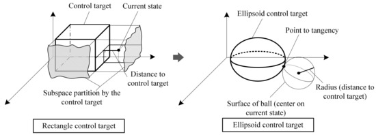
Figure 5.
The schematic of the distance to the rectangle target vs. the distance to the ellipsoid target.
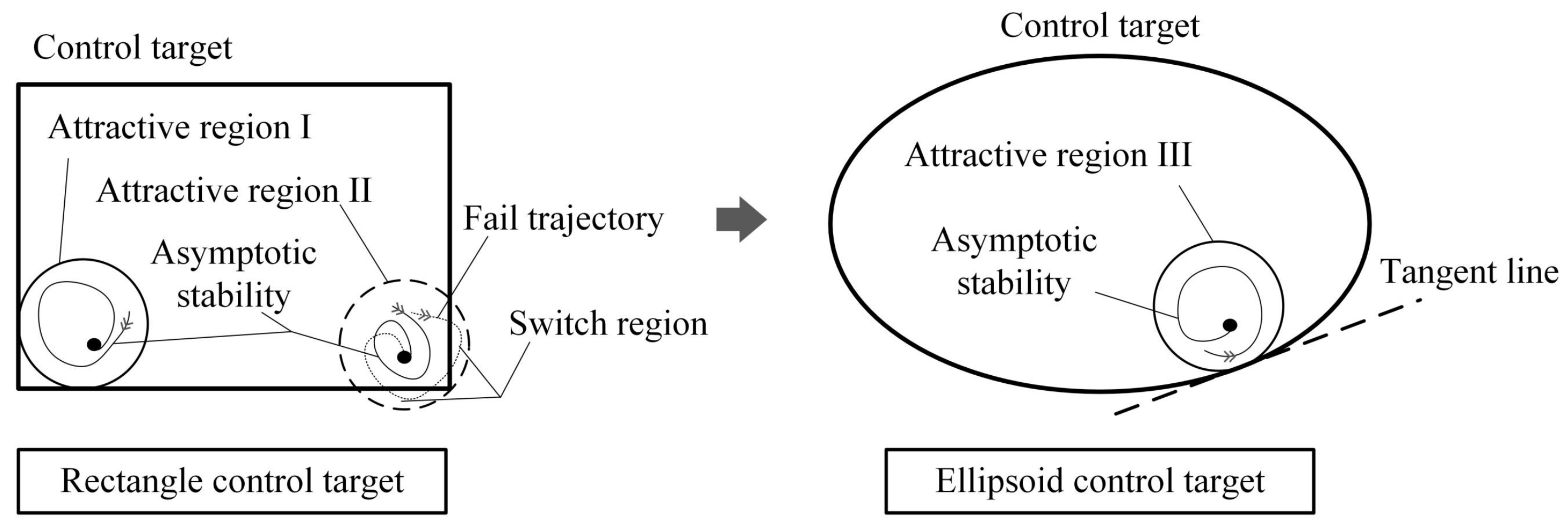
The situation changes when the control target is an ellipsoid in space. Construct a sphere in the space with the current state as the center of the sphere and gradually tangential to the space ellipsoid by gradually increasing the radius of the sphere. At this time, the radius of the sphere is the distance from the current state to the spatial ellipsoid. Since the tangent points are all on the two spherical surfaces, it can be solved by establishing a parametric equation system. This method can be referred to on the right half of Figure 5. In addition, from the perspective of asymptotic stability, the ellipsoid target can be more reasonable. When the system enters the zone target through the first phase. In order to ensure the progressive stability of the system, it is necessary to estimate a terminal attraction domain. Within this terminal attraction domain, the system can use an explicit controller to stabilize the closed-loop system along a trajectory at the optimal operating point. In Figure 6, regions I and III are safety zones, and the trajectory of the system within these zones is still inside the control target. However, Area II cannot guarantee the above requirements. The system’s trajectory may be driven out of the control target by the explicit controller, at which point the controller will switch. In this case, the system may rebuild the optimal trajectory, which represents the failure of this optimization operation. Sometimes, a high-frequency switching of the controller is also triggered, which is what controller designers do not want. To define the control target, an ellipsoid is used as shown on the right side of Figure 6. Because an inscribed ball can always be found inside the ellipsoid, and an explicit controller can be designed inside it, the running track of the system is always bounded. Therefore, a spatial ellipsoid is used as a target to avoid optimization failure. In summary, in the framework of zone control, the ellipsoid control target is more suitable than the spatial cube control target.
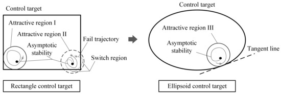
Figure 6.
The schematic of control performance of the rectangle target vs. the ellipsoid target.
In some application scenarios, a given control target is often not an ellipsoid. Therefore, an approximation is proposed to ensure that the control target can be transformed into an ellipsoid. In the above description, the general spatial cube has vertices, and the critical region that cannot satisfy the local feedback control law overlaps with these vertices. Therefore, these key areas should be replaced by smooth curves. In order to obtain a smoother boundary, a space ellipsoid can be used for replacement. The replacement target can guarantee the calculation performance and ensure the stability of the closed-loop system. In addition, the ellipsoid control target has more research results than the spatial cube. At the same time, it can also meet the needs of real industrial control, so research in this area has certain significance.
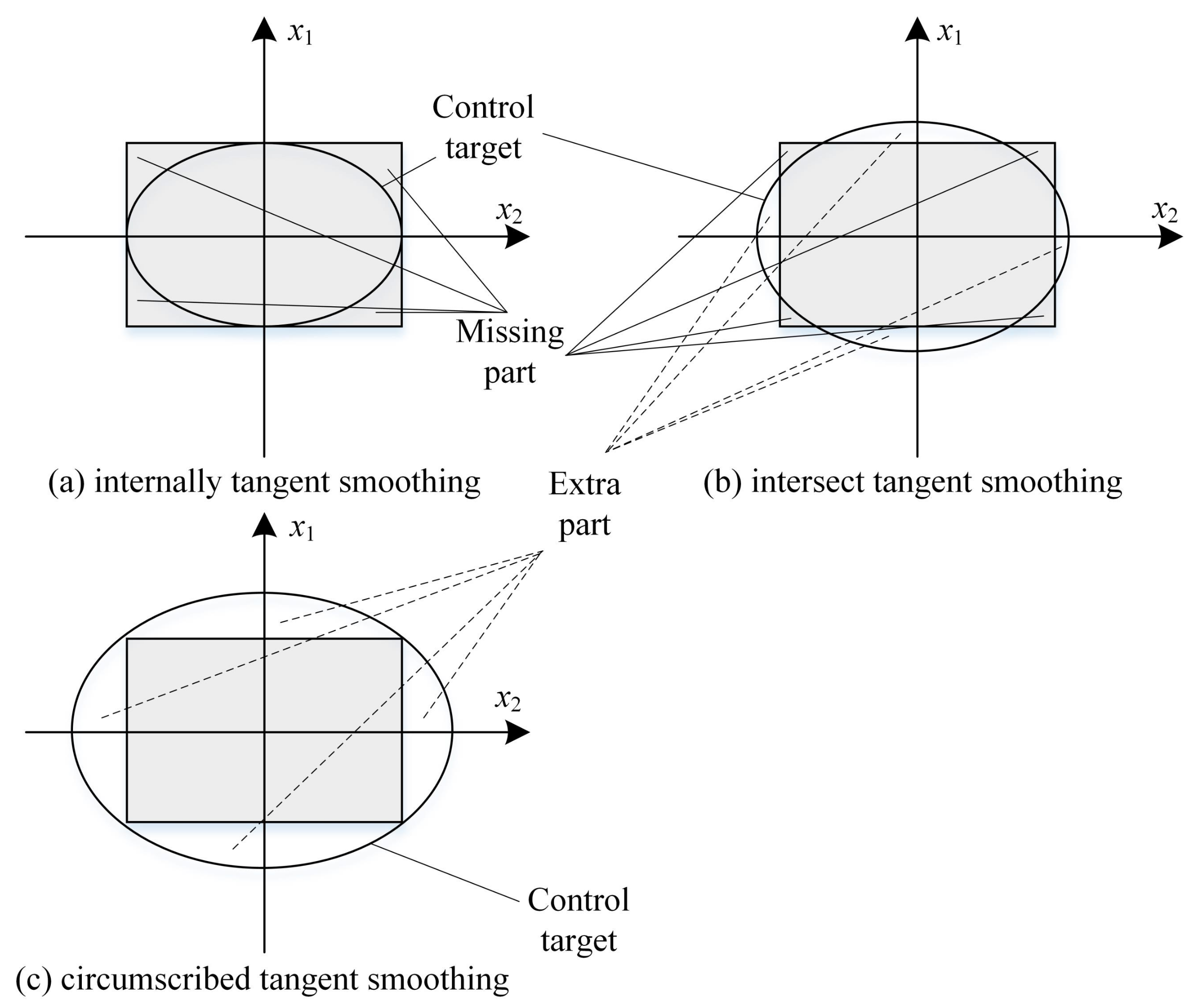
The optimization algorithm inside the model predictive control will generate large fluctuations at the boundary of the derivative discontinuity. In other words, analytic expressions are not available at the cusp, which makes the design and performance tuning of the controller difficult. From the perspective of algorithms, a quadratic programming problem with smooth boundaries has a higher efficiency. Therefore, smooth boundaries can improve the reliability of the algorithm. In a specific application, in order to make the ellipsoid target directly applicable, some approximations need to be made. Take the second-order system as an example, mainly to give a more specific description, as shown in Figure 7.

Figure 7.
Typical cases on smoothing method.
In Figure 7, method (a) employs an intrinsic approximation to reduce the actual control target. This method is suitable for control systems with stricter control targets because the set target in the controller is a subset of the original target, and the steady state of the system does not deviate from the original set target. At the same time, it can also reduce the impact of overshoot to a certain extent.
Method (b) selects a control target that intersects with the original set target. Using this method will expand or crop the original target, so one needs to weigh the advantages and disadvantages of these two control objectives in order to obtain the best results.
Method (c) is an external approximation, in which case the original control target is magnified. The resulting goal includes the original target and a portion of the additional area. This approach is applicable to non-strict control objectives, and new targets need to be accepted by process requirements.
2.3. Related Work
In zone control, a control strategy based on switching is designed. Compared with the conventional control strategy, the switching strategy can achieve higher economic benefits. Field theory is used to analyze the difference between the optimal trajectories of MPC and EMPC, concluding that the two control strategies are searching in different gradient fields. Based on these differences, a switching strategy for zone control is designed [34]. When the system state is outside the control target, MPC is employed to improve control performance. When the system state is within the control target, EMPC is utilized to enhance economic performance. Additionally, a boundary effect is present in zone control, where the input variable is manipulated by the controller to the boundary of the input constraint. To avoid boundary effects in real devices, a method is designed to project the optimal operating point at the boundary of the control target to a suboptimal operating point within the target. To improve control performance and avoid boundary effects of the system in transient or steady states, the target function of the controller is also modified. Zone control can also abstract a special class of application scenarios, such as a control system that includes margins. Margins often exist in the original design of the control system to extend the effective use of equipment. Therefore, margins are often ignored in the design process of control strategies, which can prevent the maximization of equipment performance. For example, in a heat exchange network, margins are used to optimize the control strategy, leading to improved system performance [35]. Considering margins as virtual state variables can transform conventional set point control into zone control, allowing for both economic performance and control performance to be considered in different zones to achieve overall optimal performance. Consequently, zone control, as a design tool for multivariable system controllers, can coordinate economic performance and control performance while avoiding negative effects such as boundary effects. Within the framework of zone control, margins can also be defined as redundancy [33]. The specific function of redundancy is to ensure that adjustments to a certain input variable within a small range do not affect control performance. Thus, a non-switching control strategy is developed to achieve coordination of control and optimization in the zone control system, addressing the challenge of switching on the switching surface.
3. Zone Model Predictive Control
The zone predictive control proposed in this paper is divided into two parts. When the system state is outside the ellipsoid control target, the distance measurement function is used as the performance index, which can indicate the distance between the current state of the system and the ellipsoid target. When the system state is inside the ellipsoid, the distance measurement function can be removed. However, only this distance measurement function cannot guarantee the stability of the system, so our objective function includes a finite horizon terminal constraint similar to EMPC [24]. In the framework of this paper, in order to ensure the validity of the constraints, appropriate assumptions are needed.
Assumption 2.
The applicable range of the linear model is within the ellipsoid defined by Remark 1, so the model error of the linearized model can be considered to meet the requirements.
Suppose the discrete equation of the system is shown in Equation (1) and satisfies , , where is the domain and is the range. In addition, is defined, and the steady-state operating point is defined by the following optimization problem in Equation (3).
The optimal solution of the above optimization problem can be used as the closed-loop steady-state operating point of EMPC, but the optimality cannot be guaranteed for some process control with zone control targets. The optimization problem corresponding to the classic EMPC [36] is shown in Equation (4):
where belongs to the terminal loss function. Since , let ; then, in the open-loop predicted trajectory , the open-loop trajectory can be calculated using the linearization equation. The above problems can ensure that the closed-loop trajectory of the system can obtain the optimal value under the condition of the economic loss function . However, in some process control systems, there are zone control targets , and these targets can be written as . EMPC cannot reflect the optimality of the zone target, that is, the rapidity of the system state entering the control target. To this end, a new metric is defined to indicate the distance between the current state and the set target, with the calculation method provided in Equation (5).
Therefore, the optimality or suboptimality of the distance cannot be guaranteed in a closed-loop system with an EMPC controller.
3.1. Approach to Zone Model Predictive Control
The optimization problem corresponding to the zone MPC controller can be obtained by appropriately modifying the EMPC controller. According to the proposed distance measurement index, combined with the standardized definition, the mathematical form of the zone MPC controller can be obtained.
Definition 1.
Ellipsoid control target , where .
Definition 2.
The distance represents the distance between the current state and the set target .
Definition 3.
Terminal loss function .
Based on the above definition, the optimization problem corresponding to the ZMPC controller is given as Equation (7).
where , .
3.2. Stability Analysis
In this section, the known optimal sequence is used to construct a new trajectory, which is then made to serve as a Lyapunov candidate function. The construction method is different from Grüne [25], and the method of expanding in the prediction time domain of the terminal constraint conditions is adopted. First, the behavior of the system is limited within the terminal constraints.
Lemma 2.
If there is a local controller in such that for any , then is satisfied, where .
Proof.
Therefore, can be selected so that holds; then, .
□
Theorem 1.
If there exists such that , then holds. is the objective function value corresponding to the optimal solution of the optimization problem in Equation (7).
Proof.
If is the optimal solution, it must satisfy and . So, ; then, . Assuming that there is a local controller , it can be seen from Remark 2 that . So, choose and ; then, . Therefore:
□
It can be seen from Remark 1 that a new trajectory sequence can be constructed through the optimal trajectory at time k and satisfy all constraints, where ,. Therefore, can be used as a set of feasible solutions for the optimization problem in Equation (7), that is, . And because , then . Since and, according to definitions 2 and 3, it is bounded; can be used as the Lyapunov function of the closed-loop system [37].
The performance loss function mentioned above can only guarantee asymptotic stability. Therefore, the terminal loss function is considered to be changed to another form to ensure that the system achieves strong convergence, meaning that it can enter the zone control target within a limited time.
Definition 4.
Terminal loss function [1], where P is a symmetric positive definite matrix, and belongs to the interior point of the stable feasible range, that is, is satisfied.
Lemma 3.
If the linearization system of at a steady-state operating point and its neighborhood is completely controllable, then for any , there must be a local controller that makes enter an area inside within a finite time.
Proof.
Let the linearized system at the operating point in its neighborhood as , where , . If there is a steady-state feasible region and is satisfied, the linearized system can be considered to be completely controllable [38,39] in . Let ; then, . which is
From , it follows that , so:
Let , and finally . The pole configuration can make the closed-loop system under the action of the state feedback control law satisfy all the poles of . It is inside the unit circle, where . According to the Lyapunov equation [39], if you choose a symmetric positive definite matrix Q, there must be only one symmetric positive definite matrix P so that the following equation holds.
Then select ; there is
Consider choosing so that a closed ball satisfies ; then, when , . Then, there is
So, enters the area within a finite time, and the local controller is . □
Lemma 4.
If the terminal loss function in Equation (7) is replaced by , and it is assumed that the open-loop prediction trajectory corresponding to the optimal solution of the optimization problem at time k is , then another optimal solution sequence can be constructed, and it is a feasible solution sequence of Equation (7) with as the initial value and satisfies , where , represents the value of the objective function corresponding to the optimal solution of the optimization problem in Equation (7) with x as the initial condition.
Proof.
According to Lemma 3, construct a solution sequence to satisfy , . Then, there is ; so,
In Equation (7), the terminal constraint set can be defined as the linearized neighborhood in Lemma 3. Then, the above conclusion holds, where is given by Lemma 3. □
Theorem 2.
If the optimization problem after replacing the terminal loss function in Lemma 3 is used as the controller, the state variables of the closed-loop system can enter the zone control target in a limited time.
Proof.
From Lemma 4, it is known that , and from the optimality of the optimization problem, it follows that . Thus, . Therefore, , that is, . And because , there is , that is, . Combining Lemma 3, it is known that when , the system state can enter an area inside within a limited time. Since , the system state must enter the zone control target within a limited time. Let . Then, for any , holds. □
From the above conclusion of strong convergence, it can be seen that the state of the system must enter the zone control target within a limited time. Therefore, the control algorithm proposed in this paper can ensure the stability of the zone control system.
4. Case Study
In this section, a simulation example is used to demonstrate the application of the MPC control strategy for the ellipsoid control target. To provide a more intuitive representation of the ellipsoid control target and to verify the effectiveness and stability of the proposed control algorithm, a continuous stirred tank reactor (CSTR) system is utilized to validate the ideas. Consider a lumped parameter model in Equation (16).
where the is the reaction rate constant, is the reaction activation energy (J/mol), is the ideal gas constant (J/mol·K), is the reactor volume (), C is the concentration of A in reactor (mol/L), T is the temperature of reactor (K), is the heat capacity of the mixture (J/mol·K), is the density of the mixture (), is the reaction heat (J/mol), is the inlet flow rate (L/min), is the inlet concentration of A (mol/L), is the inlet temperature (K), is the heat transfer rate of cooling water (J/min), is the cooling water flow rate (L/min), is the temperature of the cooling water (K), is the heat capacity of the cooling water (J/mol·K), Ua is the heat transfer coefficient (), is the inlet flow rate (L/min), and is the cooling water flow rate (L/min). The system’s structure is as follows in Figure 8. In this model, the variables are defined in Table 1.
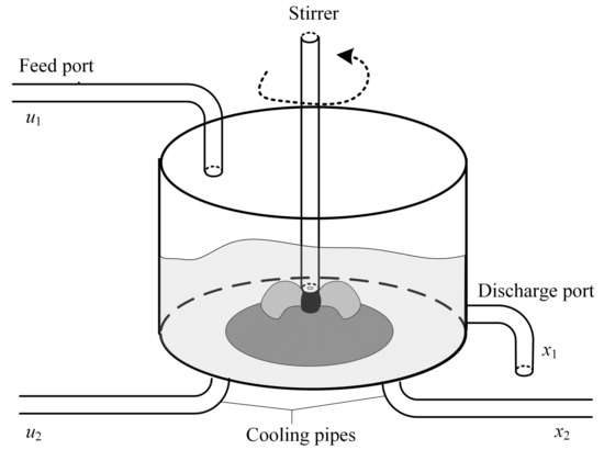
Figure 8.
Model of continuous stirred tank reactor (CSTR) system.

Table 1.
The description of each variable.
According to the invariant set theory [40] and Remark 1, a feedback matrix H exists that can ensure the satisfaction of Equation (17).
To meet the constraint condition, the linear matrix inequality is given by Equation (18).
where .
Proof.
The input constraints of the system can be expressed.
It can be rewritten as follows with state feedback matrix H.
The equivalent condition of the above inequality is as follows [41]:
With the Schur complement lemma, the linear matrix inequality can be obtained.
□
A centralized parameter model was constructed and discretized with a period of 1 min near the operating point. Without loss of generality, an unmeasurable disturbance was considered in this model. The discrete state-space model with dimensionless transformation and equalization can be described as follows:
The system constraints are as follows in Table 2.
Table 2.
The variables and constraints of the model.
Giving the initial state , control target . The requirement drives the system state into the set zone primarily and then stabilizes the system.Combined with Equation (17) and Equation (18), the appropriate state feedback matrix H can be computed as
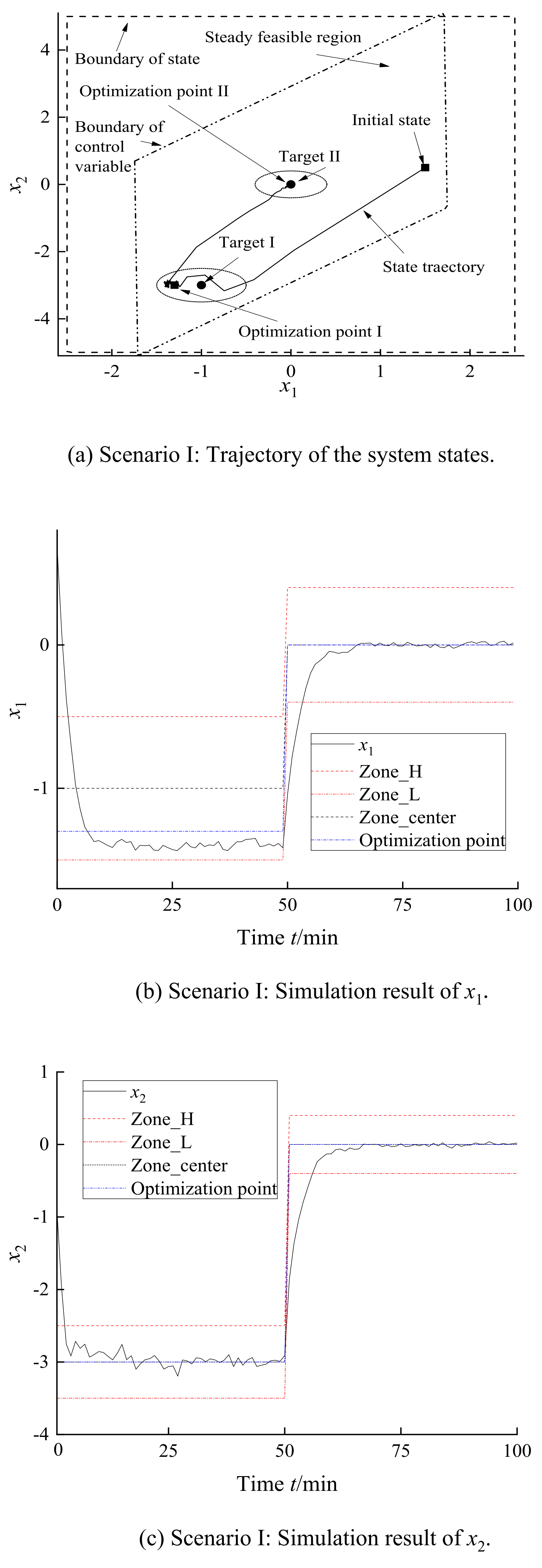
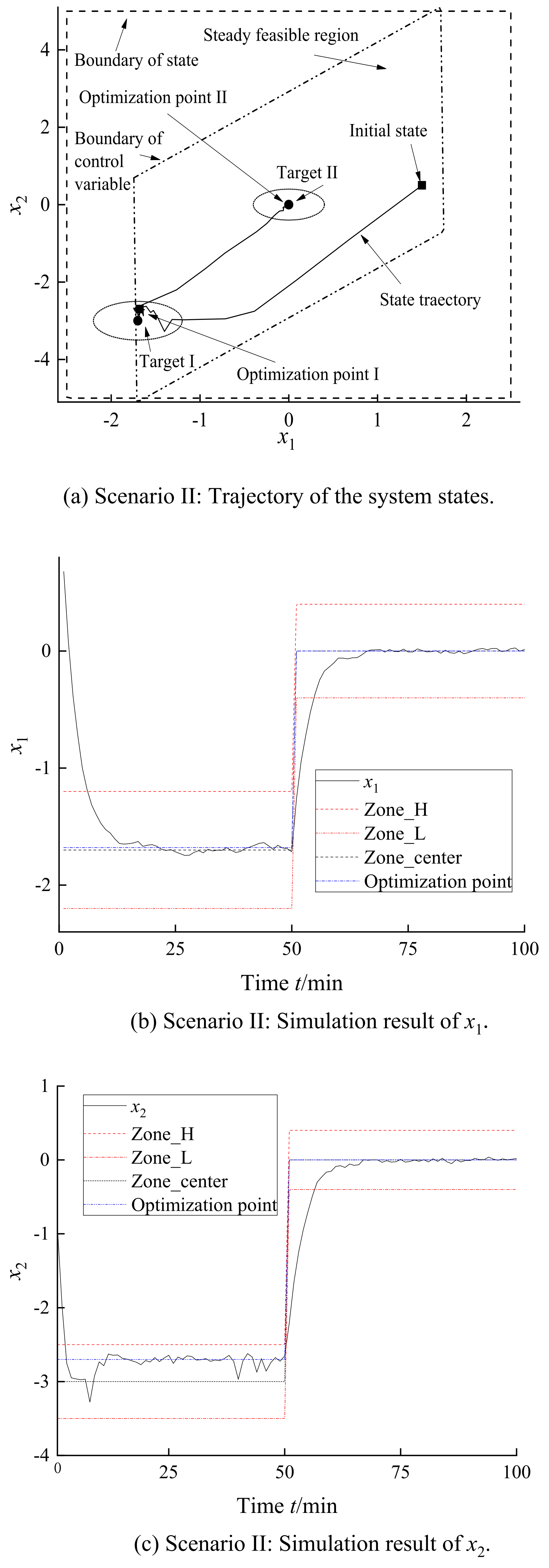
In scenario I, the predictive horizon was 10. The coefficient of zone target penalty was 10 and optimization penalty 50. The first target was an ellipsoid target whose center was and radius [0.5 0.5]. The optimization point was set to . The second target for the center was [0 0] and the radius [0.4 0.4]. The optimization point was set as the center [0 0]. The system trajectory is shown in Figure 9a. The system states can be steadied in or near the optimization point on disturbance. The system has two stages in each target. First of all, the system should be governed into the target rapidly. Then, the states should be steadied at the optimization point. As shown in Figure 9b,c, the states can be attracted into the target and then stabilized at the economic optimization point. In scenario II, the controller parameters were the same as in scenario I; however, the first target was changed in the center to and radius [0.5 0.5]. In addition, the system had the same second target with scenario I. The first optimization was set as . The system states can also be tracked by the optimization points and be governed in the set target as shown in Figure 10.
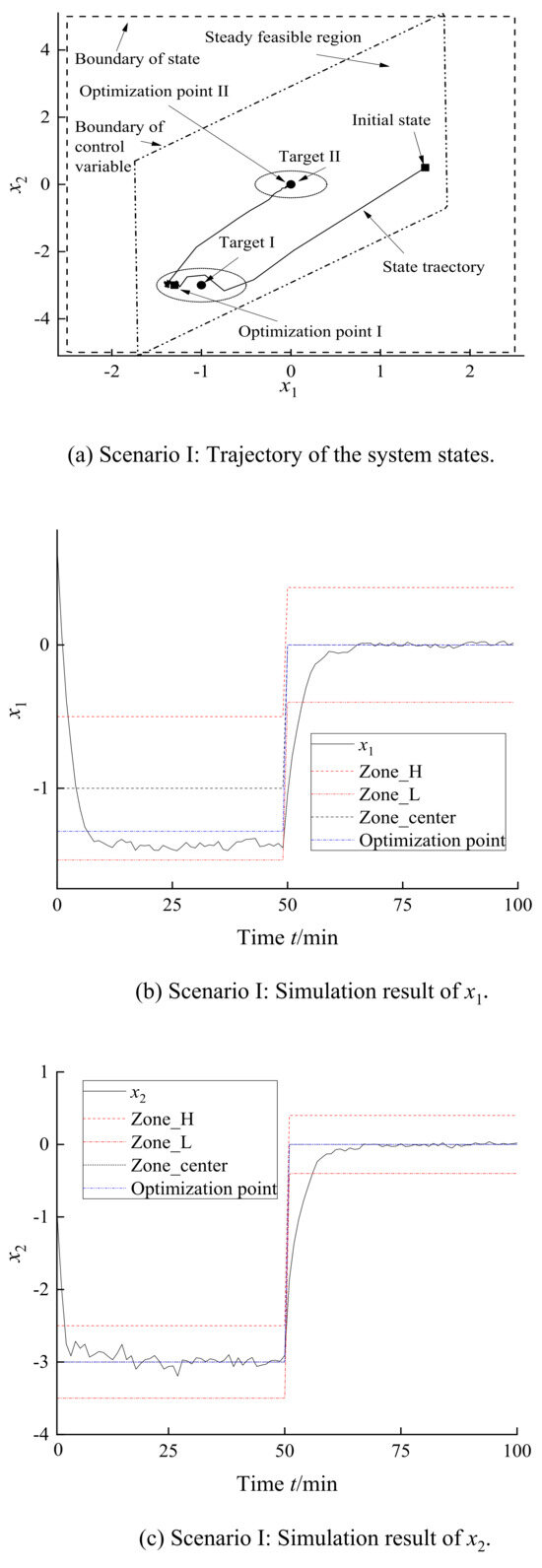
Figure 9.
Simulation results of scenario I.
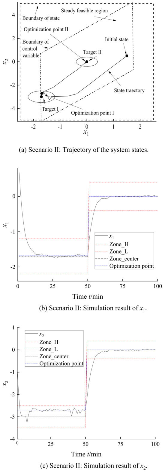
Figure 10.
Simulation results of scenario II.
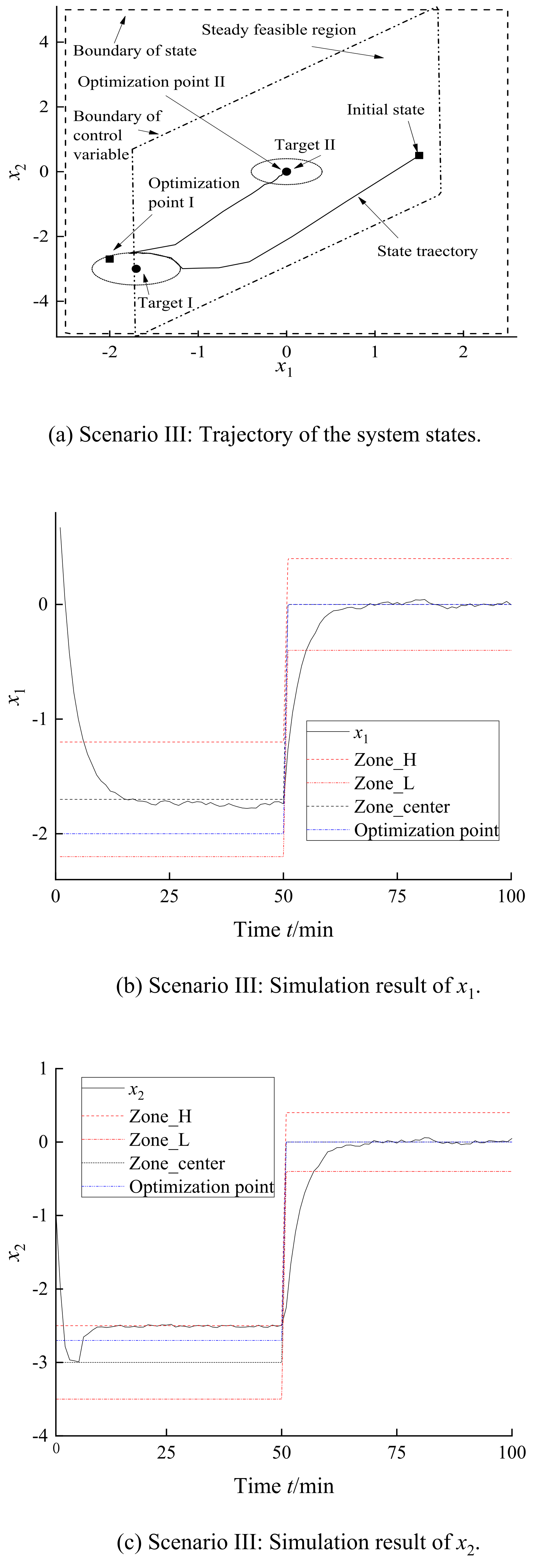
In scenario III, each parameter and target were set to be the same as those of scenario II. In addition, the first optimization point was . This point was in the first target but out of the steady feasible region as shown in Figure 11a. Therefore, the system should be steady in the boundary of the first target as shown in Figure 11c, called boundary effect. In this extreme situation, this control algorithm can also govern the system into the set target and maintain the asymptotic stability. The algorithm’s stability and control effect meet expected requirements in these three scenarios.
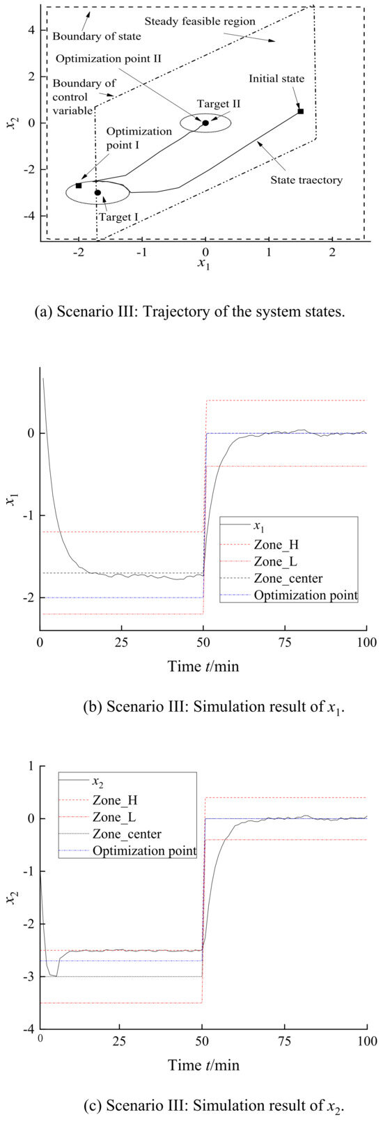
Figure 11.
Simulation results of scenario III.
5. Conclusions
In this paper, the selection of targets in the zone control task is first discussed. From the perspective of computational complexity and closed-loop control performance, it is determined that the control target should be in the form of an ellipsoid. For the design of ellipsoids, three typical methods of boundary smoothing are proposed, which can shape the space cube into an ellipsoid. A predictive control algorithm based on the ellipsoid control target is then constructed. The generalized Euclidean distance is used as the objective function of the controller and is segmented from the prediction time domain. The algorithm is subsequently deduced and analyzed, and the closed-loop asymptotic stability of the algorithm is verified. Finally, the feasibility and effectiveness of the ellipsoid target predictive control algorithm are verified using a typical CSTR model.
Future research should focus on the following three aspects: limitations of model assumptions, computational complexity, and applicability. Complex models may affect real-time computational performance, while overly simplified models could introduce significant dynamic errors. Therefore, it is necessary to address these issues comprehensively and design appropriate adjustment mechanisms to enable timely switching between different linear operating points, thereby further enhancing the control performance of the system.
Funding
This research was funded by Science Foundation of China University of Petroleum, Beijing (No. 2462021YJRC022).
Data Availability Statement
The data presented in this study are available on request from the corresponding author.
Conflicts of Interest
The authors declare that they have no known competing financial interests or personal relationships that may appear to influence the work reported in this paper.
References
- Mayne, D.Q.; Rawlings, J.B.; Rao, C.V.; Scokaert, P.O. Constrained model predictive control: Stability and optimality. Automatica 2000, 36, 789–814. [Google Scholar] [CrossRef]
- Mayne, D.Q. Model predictive control: Recent developments and future promise. Automatica 2014, 50, 2967–2986. [Google Scholar] [CrossRef]
- Sen, M.; Singh, R.; Ramachandran, R. A hybrid MPC-PID control system design for the continuous purification and processing of active pharmaceutical ingredients. Processes 2014, 2, 392–418. [Google Scholar] [CrossRef]
- Huang, Y.S.; Sheriff, M.Z.; Bachawala, S.; Gonzalez, M.; Nagy, Z.K.; Reklaitis, G.V. Evaluation of a combined MHE-NMPC approach to handle plant-model mismatch in a rotary tablet press. Processes 2021, 9, 1612. [Google Scholar] [CrossRef] [PubMed]
- Rawlings, J.B.; Muske, K.R. The Stability of Constrained Receding Horizon Control. IEEE Trans. Autom. Control 1993, 38, 1512–1516. [Google Scholar] [CrossRef]
- Grimm, G.; Messina, M.J.; Tuna, S.E.; Teel, A.R. Model predictive control: For want of a local control Lyapunov function, all is not lost. IEEE Trans. Autom. Control 2005, 50, 546–558. [Google Scholar] [CrossRef]
- Primbs, J.A.; Nevistić, V. Feasibility and stability of constrained finite receding horizon control. Automatica 2000, 36, 965–971. [Google Scholar] [CrossRef]
- Lee, Y.I.; Kouvaritakis, B.; Cannon, M. Constrained receding horizon predictive control for nonlinear systems. Automatica 2002, 38, 2093–2102. [Google Scholar] [CrossRef]
- Yu, Y.; Luo, X.; Liu, Q. Model predictive control of a dynamic nonlinear PDE system with application to continuous casting. J. Process Control 2018, 65, 41–55. [Google Scholar] [CrossRef]
- Pourdehi, S.; Karimaghaee, P. Stability analysis and design of model predictive reset control for nonlinear time-delay systems with application to a two-stage chemical reactor system. J. Process Control 2018, 71, 103–115. [Google Scholar] [CrossRef]
- Wibowo, T.C.S.; Saad, N. MIMO model of an interacting series process for Robust MPC via System Identification. ISA Trans. 2010, 49, 335–347. [Google Scholar] [CrossRef] [PubMed]
- Thombre, M.; Mdoe, Z.; Jäschke, J. Data-driven robust optimal operation of thermal energy storage in industrial clusters. Processes 2020, 8, 194. [Google Scholar] [CrossRef]
- Kadakia, Y.A.; Suryavanshi, A.; Alnajdi, A.; Abdullah, F.; Christofides, P.D. Encrypted model predictive control of a nonlinear chemical process network. Processes 2023, 11, 2501. [Google Scholar] [CrossRef]
- Dubay, R. Self-optimizing MPC of melt temperature in injection moulding. ISA Trans. 2002, 41, 81–94. [Google Scholar] [CrossRef] [PubMed]
- Oravec, J.; Bakošová, M.; Galčíková, L.; Slávik, M.; Horváthová, M.; Mészáros, A. Soft-constrained robust model predictive control of a plate heat exchanger: Experimental analysis. Energy 2019, 180, 303–314. [Google Scholar] [CrossRef]
- Ławryńczuk, M.; Ocłoń, P. Model Predictive Control and energy optimisation in residential building with electric underfloor heating system. Energy 2019, 182, 1028–1044. [Google Scholar] [CrossRef]
- Zhao, W.; Go, T.H. Quadcopter formation flight control combining MPC and robust feedback linearization. J. Frankl. Inst. 2014, 351, 1335–1355. [Google Scholar] [CrossRef]
- Dai, L.; Cao, Q.; Xia, Y.; Gao, Y. Distributed MPC for formation of multi-agent systems with collision avoidance and obstacle avoidance. J. Frankl. Inst. 2017, 354, 2068–2085. [Google Scholar] [CrossRef]
- Rahman, M.; Avelin, A.; Kyprianidis, K. An approach for feedforward model predictive control of continuous pulp digesters. Processes 2019, 7, 602. [Google Scholar] [CrossRef]
- Zhao, S.; Cajo, R.; De Keyser, R.; Ionescu, C.M. The potential of fractional order distributed MPC applied to steam/water loop in large scale ships. Processes 2020, 8, 451. [Google Scholar] [CrossRef]
- He, A.; Wang, C.; Liu, S.; Meehan, P.A. Switched model predictive path control of incremental sheet forming for parts with varying wall angles. J. Manuf. Process. 2020, 53, 342–355. [Google Scholar] [CrossRef]
- Ellis, M.; Durand, H.; Christofides, P.D. A tutorial review of economic model predictive control methods. J. Process Control 2014, 24, 1156–1178. [Google Scholar] [CrossRef]
- Adeodu, O.; Omell, B.; Chmielewski, D.J. On the theory of economic MPC: ELOC and approximate infinite horizon EMPC. J. Process Control 2019, 73, 19–32. [Google Scholar] [CrossRef]
- Liu, S.; Liu, J. Economic model predictive control with extended horizon. Automatica 2016, 73, 180–192. [Google Scholar] [CrossRef]
- Grüne, L. Economic receding horizon control without terminal constraints. Automatica 2013, 49, 725–734. [Google Scholar] [CrossRef]
- Vaccari, M.; Pannocchia, G. A modifier-adaptation strategy towards offset-free economic MPC. Processes 2016, 5, 2. [Google Scholar] [CrossRef]
- Suwartadi, E.; Kungurtsev, V.; Jäschke, J. Sensitivity-based economic NMPC with a path-following approach. Processes 2017, 5, 8. [Google Scholar] [CrossRef]
- González, A.H.; Odloak, D. A stable MPC with zone control. J. Process Control 2009, 19, 110–122. [Google Scholar] [CrossRef]
- Graciano, J.E.A.; Jäschke, J.; Le Roux, G.A.; Biegler, L.T. Integrating self-optimizing control and real-time optimization using zone control MPC. J. Process Control 2015, 34, 35–48. [Google Scholar] [CrossRef]
- Capron, B.D.O.; Odloak, D. An extended Linear Quadratic Regulator with zone control and input targets. J. Process Control 2015, 29, 33–44. [Google Scholar] [CrossRef]
- Ferramosca, A.; Limon, D.; González, A.H.; Odloak, D.; Camacho, E.F. MPC for tracking zone regions. J. Process Control 2010, 20, 506–516. [Google Scholar] [CrossRef]
- Guan, S.; Wu, X.; Wu, Z. Model predictive zone control with soft constrained appending margin. Asian J. Control 2021, 23, 2776–2785. [Google Scholar] [CrossRef]
- Wan, X.; Luo, X.L. Economic optimization of chemical processes based on zone predictive control with redundancy variables. Energy 2020, 212, 118586. [Google Scholar] [CrossRef]
- Wan, X.; Liu, B.J.; Liang, Z.S.; Luo, X.L. Switch approach of control zone and optimization zone for economic model predictive control. Chem. Eng. Trans. 2017, 61, 181–186. [Google Scholar]
- Sun, L.; Zha, X.; Luo, X. Coordination between bypass control and economic optimization for heat exchanger network. Energy 2018, 160, 318–329. [Google Scholar] [CrossRef]
- Rawlings, J.B.; Angeli, D.; Bates, C.N. Fundamentals of economic model predictive control. In Proceedings of the 2012 IEEE 51st IEEE Conference on Decision and Control (CDC), IEEE, Maui, HI, USA, 10–13 December 2012; pp. 3851–3861. [Google Scholar]
- Lyapunov, A.M. The general problem of the stability of motion. Int. J. Control 1992, 55, 531–534. [Google Scholar] [CrossRef]
- Gilbert, E.G. Controllability and observability in multivariable control systems. J. Soc. Ind. Appl. Math. Ser. A Control 1963, 1, 128–151. [Google Scholar] [CrossRef]
- Kalman, R.E. Lectures on controllability and observability. In Proceedings of the Centro Internazionale Matematico Estivo Seminar on Controllability and Observability, Bologna, Italy, 1–9 July 1968. number NASA-CR-113869. [Google Scholar]
- Kerrigan, E.C.; Maciejowski, J.M. Invariant sets for constrained nonlinear discrete-time systems with application to feasibility in model predictive control. In Proceedings of the IEEE Conference on Decision and Control, IEEE, Sydney, Australia, 12–15 December 2000; Volume 5, pp. 4951–4956. [Google Scholar]
- Boyd, S.; El Ghaoui, L.; Feron, E.; Balakrishnan, V. Linear Matrix Inequalities in System and Control Theory; SIAM: Philadelphia, PA, USA, 1994. [Google Scholar]


Disclaimer/Publisher’s Note: The statements, opinions and data contained in all publications are solely those of the individual author(s) and contributor(s) and not of MDPI and/or the editor(s). MDPI and/or the editor(s) disclaim responsibility for any injury to people or property resulting from any ideas, methods, instructions or products referred to in the content. |
© 2024 by the author. Licensee MDPI, Basel, Switzerland. This article is an open access article distributed under the terms and conditions of the Creative Commons Attribution (CC BY) license (https://creativecommons.org/licenses/by/4.0/).