Abstract
The problem of particle clogging in a conveying pipeline in thin-phase pneumatic transportation is essentially the effect of the particle-deposition mechanism in gas–solid two-phase flow. This paper presents a particle-deposition model of gas–solid two-phase flow based on the ellipsoid hypothesis, and a fast-calculation method of material particle-deposition efficiency in industry based on the tabular-assigned drag-correction coefficient of the particle ellipsoid-shape parameter and incoming flow angle . A simulation comparison of spherical particles under the same pneumatic transport conditions and experimental verification based on the self-built particle deposition system are given. The validity of the model and the accuracy of the algorithm are verified. This provides a feasible simulation and experimental scheme for the research of pneumatic-conveying technology in the industrial field.
1. Introduction
Pneumatic conveying is a fluidization technology application that uses air flow with a certain pressure and speed to transport powdery bulk materials. Because of its stable work, strong sealing, no material pollution, and high level of automation of the conveying process, it is widely used in process engineering. As the most traditional method of pneumatic conveying, thin-phase pneumatic conveying has low pipeline pressure and mature technology. It undertakes important raw-material conveying tasks in chemical, electric power, gold control, building materials, and other industries. The flow rate of the thin-phase pneumatic-conveying air flow is high, generally greater than 12 m/s, the porosity of the material is large, and the material–gas ratio volume ranges from 1:20 to 1:50 [1,2]. It is essentially the specific migration and application of the gas–solid two-phase flow theory. A large number of scholars have explored the law of particle migration and deposition in the gas–solid two-phase flow, promoting the development of thin-phase pneumatic-conveying technology. Among them, the transportation pipeline, as the main component to ensure the stable transportation of thin-phase gas, has received widespread attention for studying and solving the problems of blockage of conveying materials and local dead zones.
Ebrahimi M. et al. [3] carried out experimental and simulation studies on thin horizontal pneumatic conveying. The results indicated that, within the range of mass solid-loading ratios from 2.3 to 3.5, the larger the particle diameter, and the higher the solid-loading ratio, the lower the particle velocity. Ebrahimi M. et al. [4] conducted a comparative study on the alteration of the predictive capacity of turbulence models considering source terms in the regulation of particles in horizontal pneumatic transport, within the framework of a CFD-DEM Eulerian–Lagrangian simulation. Bhattarai S. et al. [5] simulated the alterations of wind pressure, wind speed, temperature, and particle water content in the pneumatic-conveying drying process of wood chips when the inlet temperature of hot air was fixed at 100 °C, and offered engineering suggestions that the rational utilization of buffers could effectively enhance the drying efficiency. However, the above studies are all based on the spherical particle hypothesis. Although the numerical model of gas–solid two-phase flow is simplified, it cannot accurately describe the particle shape elements in the transportation process, nor can it accurately characterize the particle–particle and particle–wall collision characteristics during transportation. To this end, more scholars have adopted discrete unit methods that can more accurately capture the motion state of material particles and clearly describe the collision process between particles and the wall to research thin-phase pneumatic-conveying pipelines.
Zhou [6] adopts the discrete-unit coupling method from the conveying flow state. The particle distribution and other aspects studied the particle transport characteristics of the co-flow pneumatic-conveying process of coarse-heavy particles and light-medium particles and the evolution process of the material plug. Almeida [7] used the discrete-unit coupling method to simulate the pneumatic separation of bagasse particles, and gave experimental verification. Xu [8] gave suggestions for the optimization design of wheat pneumatic-conveying equipment considering the material collision angle and the bending diameter ratio of the transportation elbow. Guzman [9,10] studied the relationship between the solid loading ratio of pea seeds at different pneumatic flow rates and factors such as sowing speed, seed collision, and elbow diameter. With the gradual deepening of the research on the characteristics of the thin-phase pneumatic-conveying process, the advantages of the discrete-element coupling method have become more and more obvious, but the calculation amount is too large, the calculation cost is too high, and the grid quality, drag and take complex factors mean that the method is limited in engineering application [11].
In this paper, ellipsoidal particles that can better capture the motion characteristics of some non-spherical particles such as discs, fibers, cylinders, etc. are used as hypotheses for the morphology of material particles to study the sedimentation distribution of material particles in thin-phase gas transportation [12]. Firstly, the calculation table K of the ellipsoidal-particle drag correction factor considering the axial length ratio and spatial orientation of the ellipsoid is established, based on the classical channel flow model to offer parameters for the rapid calculation of the particle deposition distribution during thin-phase pneumatic transportation. Then, the ellipsoidal-particle deposition model is established by Fluent, in combination with the drag correction-coefficient-K assignment table, and the calculation process of the deposition efficiency is provided. Simultaneously, the experimental platform for particle migration and deposition was constructed to validate the particle migration and deposition of silica samples. Finally, the simulation results of the ellipsoidal particle hypothesis and the spherical particle hypothesis are compared with the experimental results under the same pneumatic transport conditions.
2. Ellipsoidal-Particle Deposition Model
2.1. Ellipsoidal Particle Appearance
Through the super-quadratic surface equation, the topological characteristic description of symmetrical spherical particles that can characterize the spatial orientation is realized. It allows us to describe the geometric shapes of convex and concave shapes, and its functional form can be expressed in Formula (1) as
where and are the shape parameter, which characterizes the sharpness of different spaces; is the x–z and y–z planes of space, is x–y planes; and , and are axial lengths in the x, y, and z directions, respectively.
For the particles studied in this article, , spherical and ellipsoidal particles can be described. The ellipsoidal particles considered in this section can be described by to simplify Formula (2)
In order to better characterize the shape characteristics of symmetrical spherical particles, rather than emphasizing the particle size scalar, the axis-length ratio is introduced, which is expressed as the ratio of the length of the half-axis of the rotary axis in the x-axis direction and the length of the half-axis of the equatorial axis in the y-axis direction , as shown in Formula (3).
When , the symmetrical spherical particles show an elongated shape in the x-axis, and when , the symmetrical spherical particles show a flat shape in the x-axis.
When , the above formula can be used to describe spherical particles.
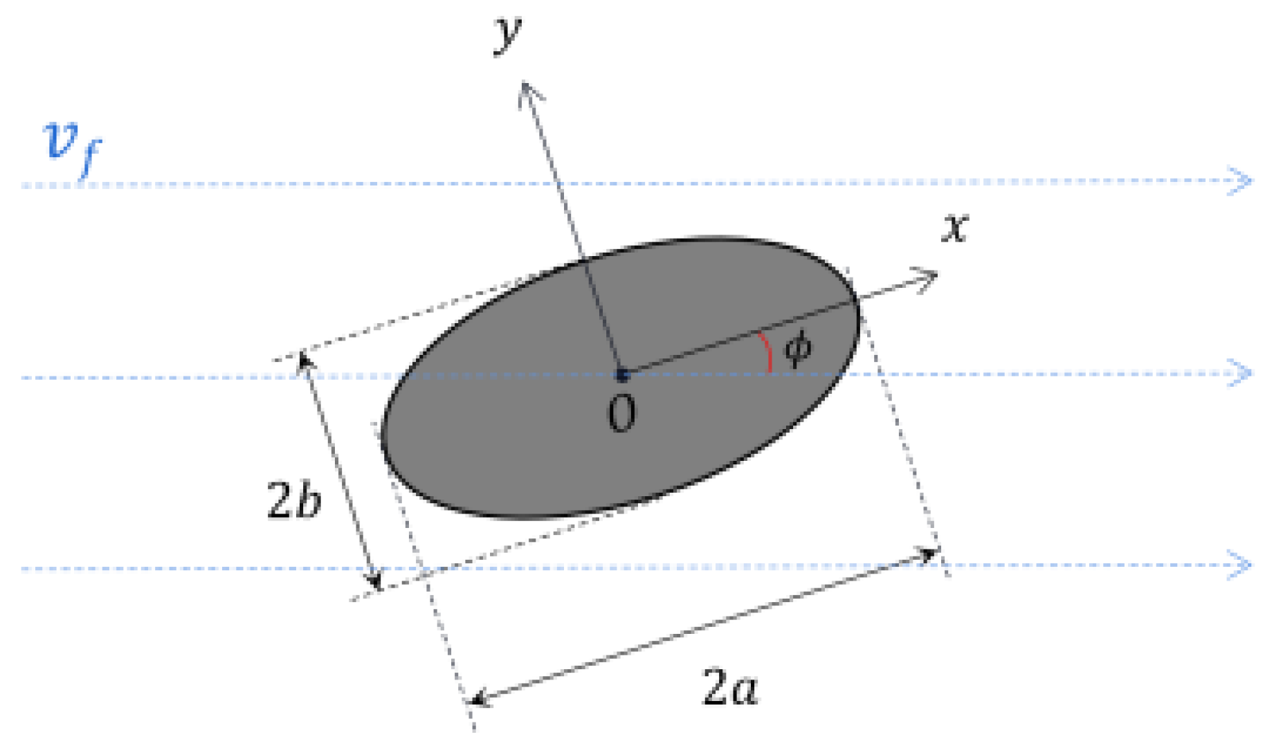
According to the above description, the migration morphology of symmetrical spherical particles in the fluid can be characterized according to Figure 1, in which the angle between the particle rotation axis x and the continuous phase fluid is used to characterize the spatial orientation of the particles. The x-axis (rotary axis) and y-axis (equatorial axis) are the main axes of the x and y directions of symmetrical spherical particles, respectively, and the angle between the incoming flow is located in the x-y plane, where the particles are located. When , it means that the rotation axis of the symmetrical spherical particles is consistent with the flow direction of the continuous phase fluid; and when , it means that the rotation axis of the symmetrical spherical particles is perpendicular to the flow direction of the continuous phase fluid, wherein when , the particles correspond to spherical particles, there is no spatial orientation, and set .
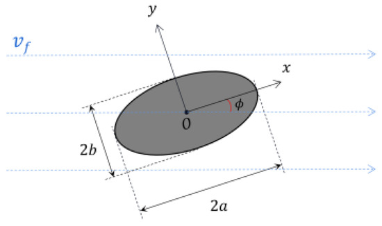
Figure 1.
Motion morphology of symmetric spherical particles.
2.2. Ellipsoidal-Particle Drag Correction
2.2.1. Obtaining of the Drag-Force Correction Coefficient
According to the drag force of ellipsoidal particles mentioned earlier, depends on the Reynolds number, the complex relationship between the axis-length ratio of ellipsoidal particles and their spatial orientation; it is difficult to achieve accurate estimation of the drag force of ellipsoidal particles with different axis-length ratios through various existing empirical formulas and theoretical derivations. In order to better describe the drag force of ellipsoidal particles and equal-volume spheres under the same Reynolds number conditions, the drag-force correction coefficient is introduced, as described in Formula (4).
where represents the drag force of spherical particles of the same volume as symmetrical spherical particles under the same Reynolds number conditions.
The channel flow model based on the immersion boundary method is simulated and solved. The spectral element method will be used in combination with the open source platform Nek5000 to numerically simulate the ellipsoidal drag coefficient for a given specific particle-motion-morphology parameter method, so as to obtain the precise value of the drag force of the ellipsoidal particles under the specific parameter setting.
The symmetrical sphere is placed in the center of the channel, and the fluid is allowed to flow stably around the symmetrical sphere. It simulates the drag force of ellipsoidal particles at different incoming flow velocities, various symmetrical sphere shapes, and various incoming flow angles (also known as flow angles of attack). The channel adopts a uniform-velocity inlet condition, the wall surface is the slip boundary, and the inlet moves at the same speed, that is, the boundary condition without shear stress. The outlet uses natural outflow conditions, that is, the vertical velocity gradient is zero. Through the above-mentioned conventional boundary condition setting, the finite-space truncation method within the flow range of the channel is realized to simulate the infinite boundary problem in the gas–solid two-phase flow. By defining the values of typical parameters, the drag coefficient of ellipsoidal particles under typical conditions is solved, as shown in Table 1.

Table 1.
Morphological parameters of ellipsoidal particle motion.
Among them, the selected values of the aspect ratio parameter represent ellipsoidal particles that show a flat shape on the x-axis ( = 0.5, that is, 2 a = b = c), and two ellipsoidal particles that show different elongated forms ( = 2, that is, a = 2 b = 2 c and = 4, that is, a = 4 b = 4 c) and spherical particles ( = 1, that is, a = b = c). The numerical selection of the angle parameter between the incoming flow represents the spatial orientation state of the ellipsoidal particles consistent with the direction of the incoming flow ( = 0°), vertical ( = 90°), and the remaining two typical angles ( = 30°, 60°). The determination of the Reynolds number range considers the parameter settings in pneumatic transportation engineering, as documented in Reference [13], and when combined with the Reynolds number calculation in Formula (5), yields a distribution primarily encompassing orders of magnitude such as 100, 101, 102 and 103.
For the external flow considered in this manuscript, and represent the fluid density and dynamic viscosity coefficients. For air at normal pressure, the density at 20 °C is 1.204 kg/m3, and the aerodynamic viscosity is approximately 1.5 × 10⁻⁵ m2/s. and are the velocity of the incoming flow from the far front and the particle size of the material. The velocity of the pneumatic transport for the thin phase ranges from 101 to 102, and the material size varies from 10−4 to 10−5, as documented in Reference [13].
Meshing uses the open-source three-dimensional finite-element mesh Gmsh program to generate three-dimensional geometric models of different examples described in Table 1 through the script language; the mesh is discrete, and can realize the O-shaped mesh wrapping of ellipsoidal particles in the tank flow model, and the distortion or intersection of overlapping mesh areas. The problem is automatically coordinated and interpolated.
By setting rational wall parameters, flow field space and turbulence parameters, filter operators, etc., the joint calculation of the nodes in the cell is accomplished through the utilization of the spectrum element method simulation and development platform jointly compiled by C and Fortran. After solving, the values of the drag correction coefficient K corresponding to different aspect ratios , Reynolds number , and the angle between the incoming and outgoing currents are obtained, as shown in Table 2.
Table 2.
Comparison table of drag correction coefficients of symmetric spherical particles.
2.2.2. Analysis of the Drag-Force Correction Coefficient
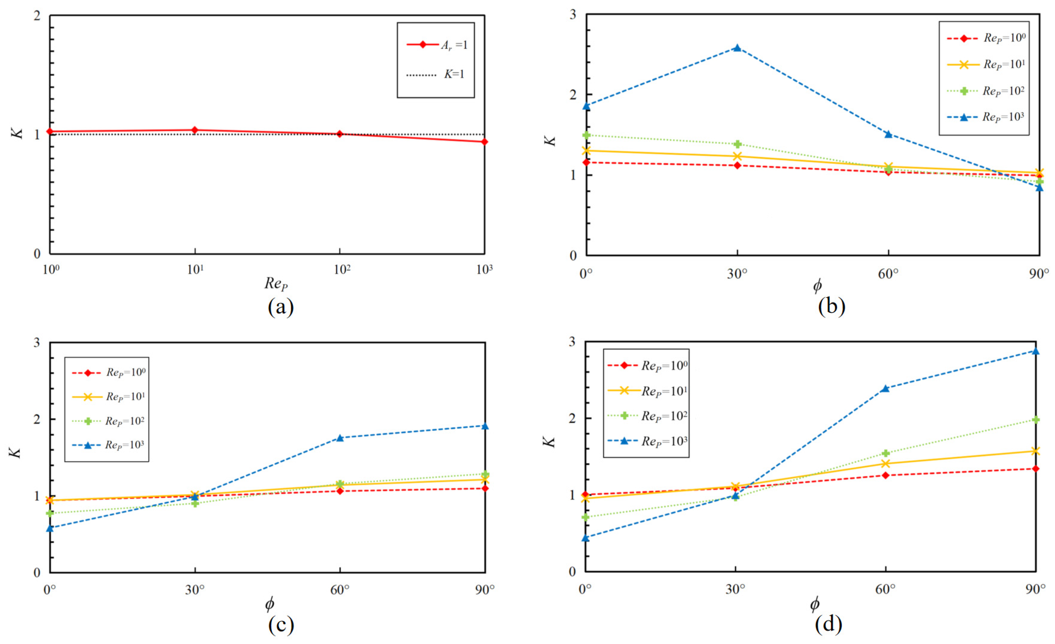
In order to verify the feasibility of the numerical simulation method of drag of ellipsoidal particles described earlier, in Figure 2a, the drag correction-coefficient results of spherical particles ( = 1, = 0°) under the Reynolds number of different particles in Table 2 are given. It shows the theoretical value line (K = 1) of the drag correction coefficient for spherical particles ( = 1). By comparing and simulating the drag correction coefficient obtained under the conditions of = 100, 101, 102, and 103, the relative errors are 2.5%, 3.7%, 0.4% and 6.2%, respectively, which accord with the error estimation range of the empirical formula for drag calculation.
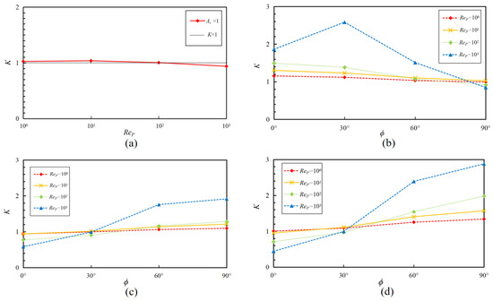
Figure 2.
Simulation diagram of drag correction coefficient. (a) Correction coefficient under various Reynolds numbers ( = 1); (b) correction coefficient of flat symmetric spherical particles ( = 0.5); (c) correction coefficient of elongated symmetric spherical particles ( = 2); (d) correction coefficient of elongated symmetric spherical particles ( = 4).
The simulation results of drag correction coefficients for ellipsoidal particles ( = 0.5, 2, 4) at different inflow angles ( = 0°, 30°, 60°, 90°), different Reynolds orders of magnitude ( = 100, 101, 102, 103), and in flat and elongated shapes along the x-axis are presented in Figure 2b–d.
As can be seen from Figure 2b, when the flat ellipsoidal particles are at 100 ≤ ≤ 102, the drag correction coefficient of each particle under the Reynolds number condition decreases with the increase in the angle between the incoming flow. This phenomenon is mainly due to the fact that the eddy-current differential pressure force in the drag force of the particles gradually decreases with the change in particle morphology, and the ellipsoidal particles that show a flat shape in the x-axis show a smaller windward area as the angle between the particles and the incoming flow increases. With the increase in the Reynolds number of the particles, the dominant influence of eddy pressure differential force becomes more pronounced, and under the condition of the Reynolds number of particles of the order of = 103, the ellipsoidal particles with a flat form at = 30° have a rapid increase in the drag-force correction coefficient, and then with the gradual increase in the angle between the incoming flow, the conventional trend of decreasing is restored. This is mainly due to the fact that, under the condition of a large Reynolds number, the fluid flows and separates at the inflow of flat ellipsoidal particles with a certain spatial orientation. The fluid produces a greater negative pressure at the inflow, resulting in a larger inverse pressure gradient at the space of the particle symmetrical body, which leads to the formation of turbulence or eddies in the fluid. The air bubbles are separated, resulting in a sudden increase in drag. As the angle between the incoming and outgoing flow continues to increase, the fluid separation point gradually moves in the direction of the flow along the outer edge of the ellipsoidal particles, and gradually decreases after reaching the maximum drag value.
In contrast to ellipsoidal particles with flat forms, ellipsoidal particles with slender forms on the x-axis, under the set Reynolds number conditions of each particle, the drag-force correction coefficient increases with the increase in the angle between the incoming flow. This phenomenon is mainly due to the fact that the eddy-current differential pressure in the drag force of the particles varies with the particle shape. The change gradually increases, and the ellipsoidal particles that take on an elongated shape in the x-axis show a larger windward area as the angle between the incoming and outgoing currents increases. This change increases with the increase in the particle Reynolds number, and the dominant role of the eddy-current differential pressure force becomes more significant, as shown in Figure 2c.
For slender ellipsoidal particles with = 4, under the set Reynolds number conditions of each particle, the trend of change in the drag correction coefficient is similar to that of slender ellipsoidal particles with = 2. It also shows a law of change that increases with the increase in the angle between the incoming and outgoing currents, and as the particle Reynolds number increases, the dominant effect of the eddy-current differential pressure becomes more significant. However, its rate of change is significantly higher than that of the former. At the order of = 100, the drag correction coefficient of = 4 slender ellipsoid particles with an angle of 90° from the flow is 1.34 times that of the angle of 0° from the flow, and the drag correction coefficient of = 2 slender ellipsoid particles is 1.17 times; on the order of = 103, the drag correction coefficient of = 4 slender ellipsoidal particles with a flow angle of 90° is 6.5 times that of the flow angle of 0°, while the drag correction coefficient of = 2 slender ellipsoidal particles is doubled by 3.3 times. Combined with the numerical calculation results of the drag correction coefficients of other incoming flow angles, as shown in Table 2, it shows that under the same particle Reynolds number, the drag correction coefficients of ellipsoidal particles with an elongated shape on the x-axis increase monotonically with the increase in the incoming flow angle, and the axis-length ratio affects. The weight of the drag force correction coefficient also increases non-linearly, and the characteristic that the eddy-current differential pressure force gradually plays a significant role with the increase in the particle Reynolds number is further verified, as shown in Figure 2d.
2.2.3. Mathematical Model of Flow Field
In this paper, the renormalization group k-ε (RNG k-ε) turbulence model commonly used in the field is used to simulate the time-averaged flow field, and its higher adaptability to the strain rate and the applicability of the streamline bending degree are used to fit the flow characteristics of particles affected by the insufficient development of near-wall turbulence during the migration and sedimentation process. In the RNG k-ε model, k and ε can be described as
where is fluid density, is the velocity vector, is the effective dynamic viscosity, is the turbulent kinetic-energy generation term, and are, respectively, the reciprocal of the effective Prandtl number and , and are empirical constants, and serves as the source expression of .
2.3. Ellipsoidal-Particle Deposition Model
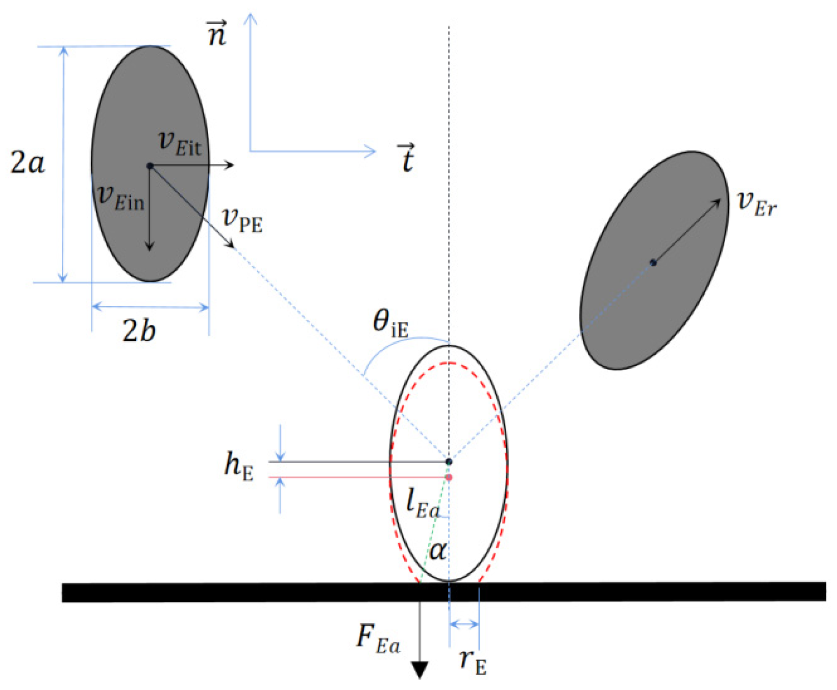
In the simulation process of thin-phase pneumatic conveying, the material particles are assumed to be ellipsoidal particles relative to spherical particles. Because of the specificity of their geometry, the movement process will be more complicated [14], and there may be a variety of movement methods, such as constant movement, periodic movement, tumbling, and mixing [15]. However, before entering the near-wall area of the fluid, the fluid area is wide enough, relative to the ellipsoidal particles. If the particles can rotate freely, the final stable orientation will be the direction with the greatest resistance [16,17]. According to Table 2, it can be seen that, at this time, for < 1 the flat particles are stable to the angle of the flow with the greatest resistance being = 0°, and the slender particles of > 1 are stable to the angle of the flow with the greatest resistance being = 90°. At this time, the process of collision between the ellipsoidal particles and the particle deposition wall is shown in Figure 3, where represents the adhesion angle.
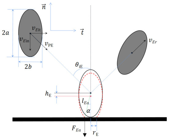
Figure 3.
Symmetric spherical-particle–wall collision escape process.
The determination of the deposition and desorbed state of ellipsoidal particles depends on the direction and size of the torque of the force acting on the surface of the particles. Among these, the direction of adhesion moment and gravity moment is counterclockwise, acting to maintain the adhesion of the particles to the wall of particle deposition; and the drag moment and collision moment are clockwise, acting to detach the particles from the wall.
In the formula, is the acceleration due to gravity, and is the surface energy between particles; is the linear distance between the symmetric spherical center point and the adhesion point, shown as Figure 3; and , , and are the equivalent Young’s modulus, the effective contact radius of curvature, and the equivalent mass, which can be expressed by the following formula.
where is fluid density, is particle density, is Poisson’s ratio of particulate matter, is Poisson’s ratio of the dust accumulation, is the elastic modulus of the dust accumulation, and , , and are the elastic modulus, the radius of curvature, and the mass of the deposited wall. So, when , the particles will show desorbed motion after the collision; otherwise, the particles will be deposited on the wall.
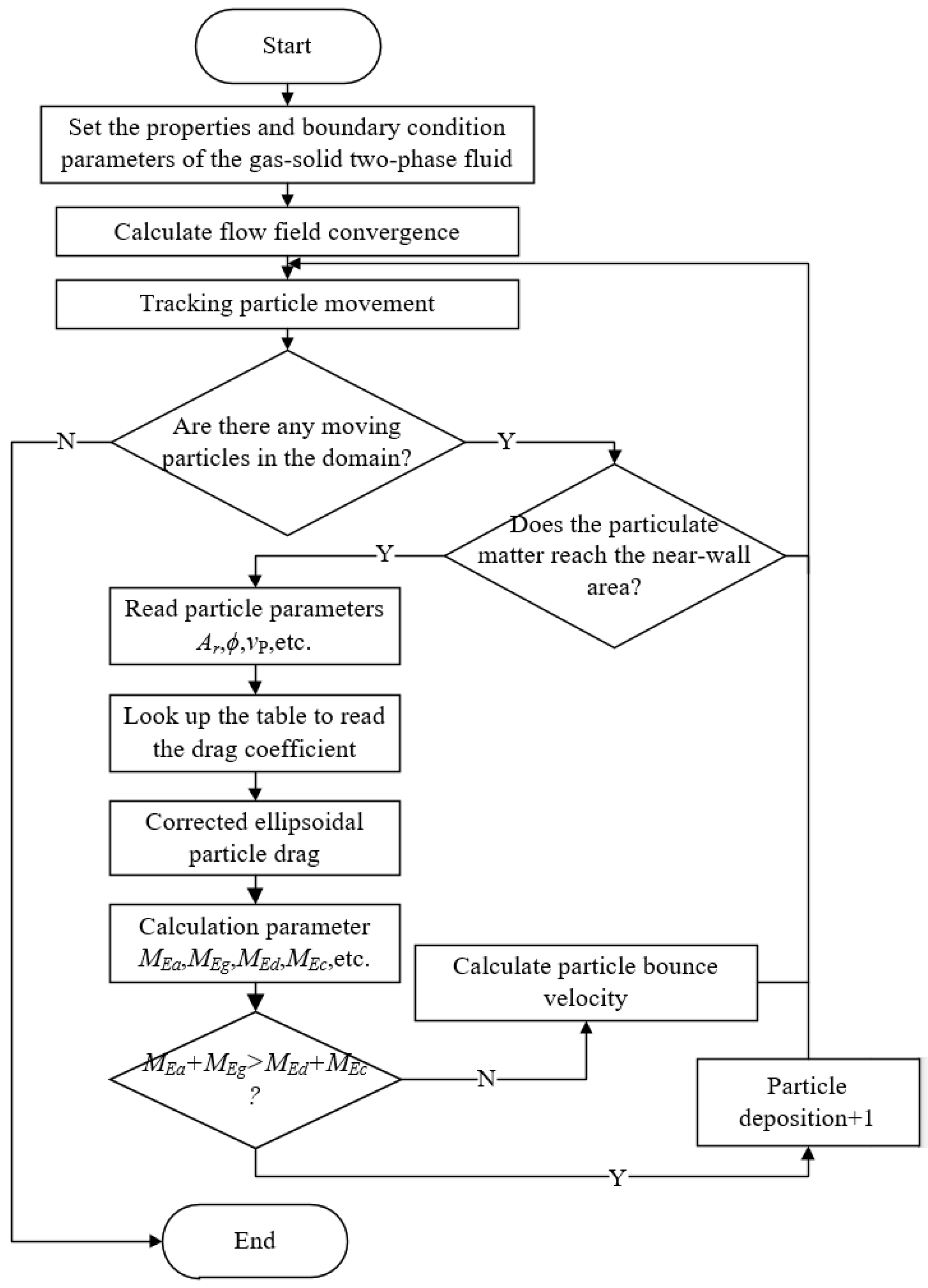
The specific calculation-process steps are shown in Figure 4.
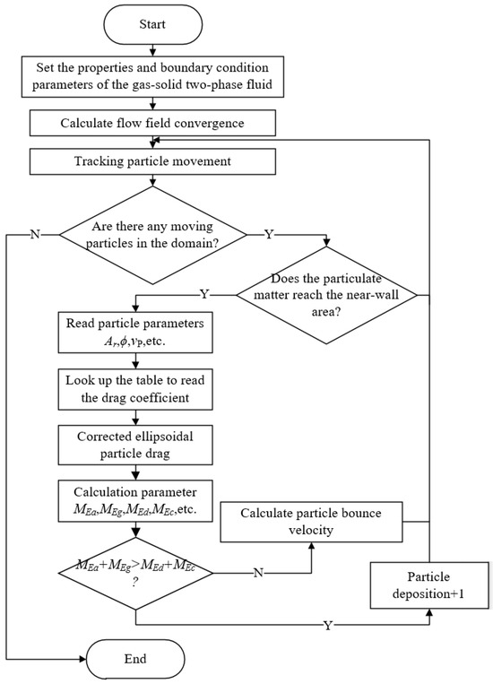
Figure 4.
Calculation flow chart of spherical particle-migration model in flow field.
The ellipsoidal particle-migration model in the flow field established in this chapter employs Fluent to analyze the gas–solid two-phase flow field based on the Euler–Lagrange method through setting parameters such as the properties of the gas–solid two-phase fluid, boundary conditions, and other condition functions like the criteria for particle deposition and desorption in UDF transmission. Subsequently, the drag force and other force-condition functions are corrected in accordance with the input ellipsoidal particles. The motion trajectory of the particles within the calculation domain is captured, and the motion or deposition state of the particles is analyzed in accordance with the sedimentation criteria proposed in this paper.
3. Results
3.1. Particle Migration and Deposition Simulation
Coupling the two-parameter particle-probability-deposition model with the solver of commercial fluid calculation software ANSYS FLUENT 2021 R2, a long straight pneumatic-conveying pipeline of 0.6 m × 0.6 m × 30 m (L = 50 D) was selected as the background space, and, based on the discrete-phase model (DPM), the working wind speed and air were regarded as the continuous phase, and the transported silica-particle material is regarded as a discrete phase. In order to obtain a faster convergence velocity, the coupling of pressure and velocity is calculated by using the SIMPLE algorithm, and the discrete form adopts the standard method, except for the pressure term, and the rest of the convection term and viscous term are discretized by the second-order welcome style.
Among these, the wind speed of the working conditions is based on the thin-phase pneumatic-conveying velocity, and the parameters of the air velocity in the simulated working conditions are set for 12 m/s. Material particles selected are common industrial raw-material silica, with a particle size of 40 µm.
3.2. Particle Migration and Deposition Experiment
3.2.1. Experimental Platform for Particle Migration and Deposition Simulation
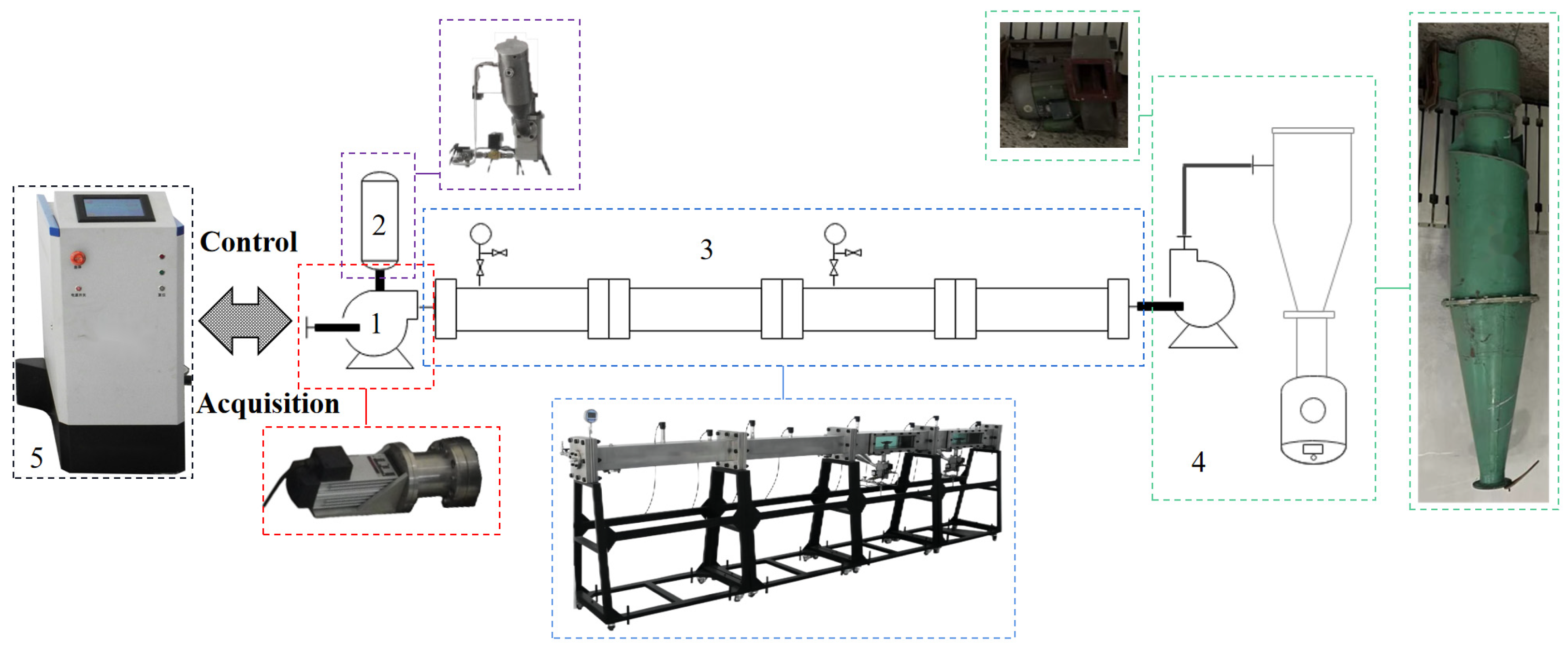
Based on the experimental platform for particle migration and deposition simulation, the micron-scale pollution-particle migration and deposition test was carried out under working conditions, and the experimental platform is shown in Figure 5.
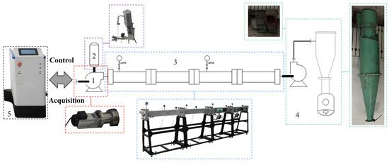
Figure 5.
Experimental platform for particle migration and deposition simulation. 1—Flow field generator; 2—particle disperser; 3—particle-sedimentation migration pipeline; 4—particle collection system; 5—multi-channel data-acquisition controller.
In order to achieve the simulation of the whole process of particle migration, it is equipped with a flow-field generator equipped with an explosion-proof fan. The fan speed is adjustable from 0 to 6000 rpm and the blades can be replaced. Through a suitable ratio, it can provide a uniform working condition of 0~15 m/s in the inlet section. Environmental wind-speed experimental conditions can be set for particles with the deflector. The experimental simulation of migration and deposition provides a stable flow-field environment [18].
The particle disperser is equipped with a gas-phase agitation device composed of four magnetic fans at different angles to each other, and is used to fully and evenly disperse a large volume of gas–solid two-phase flow. During the test, the particles are injected into the cavity through a V-shaped particle deflector under micro-pressure to achieve the uniform dispersion of the particle input.
The particle transport and deposition pipeline adopt a segmented design, and the main body of the pipeline is a double-layer stainless steel structure with a square section, which can be freely connected through flanges and angle adapters. The inner diameter of the nozzle D = 150 mm; showing a square section, the length of each section L = 10 D= 1500 mm, and the maximum working pressure is 4 MPa. The pipeline can be divided into two types: an optical-observation pipeline and an optical-measurement pipeline. Among these, the optical-observation pipeline has two pairs of circular optical-glass observation windows with an opening diameter of 90 mm, two groups of temperature- and pressure-acquisition sensors and one group of hot-wire wind-speed-acquisition sensors. Meanwhile, it is equipped with a precision proportional gas-distribution device, pressure-relief bursting disc, and multiple groups of detachable installation flanges for detecting the expansion of sensors. The optical-measurement pipeline is provided with four-way omni-directional optical-glass visible windows, which are respectively arranged at the upper- and lower-wall surfaces and the left- and right-wall surfaces of the pipeline in the middle position; each group of optical windows is strictly parallel; the window size is 1200 mm × 135 mm; high-purity fused-silica glass is adopted; the transmittance is greater than 90 percent; the transmission wavelength range is 200–1000 nm; the surface accuracy is 1/4 wavelength (328 nm); and the optical detection conditions such as particle velocity measurement and the like can be met [19]. In addition, each pipeline is equipped with a particle-deposition collection plate and an installation groove, which can be used to change the roughness of the pipe wall, the material of the pipe wall and the morphology of the collected particle deposition [20,21].
The particle collection system consists of a centrifugal fan, a cyclone dust collector, a gas–liquid separation device, and an exhaust-gas filtration device, which can realize the pollution-free collection and discharge of experimental particles, waste liquid, and exhaust gas.
A multi-channel data-acquisition controller, with 12-channel synchronous data acquisition function, a maximum sampling time of 6 s, and a sampling time interval of 0.2 ms, can realize the electrical access of sensing signals, such as pressure, temperature, wind speed, vibration, flame light, etc. and the accurate control of external-trigger acquisition systems such as electromagnetic-flow valves and high-speed cameras. Equipped with a remote start controller and wireless data-transmission module, it can realize the remote start and stop of particle migration and deposition experiments.
3.2.2. Test Samples
The sample parameters of the silica (SiO2) particles used in the experiment are shown in Table 3.
Table 3.
Sample parameters.
Sample pretreatment is as follows:
(1) Cleaning and pretreatment: the experimental samples of silica (SiO2) particles are first dissolved with acetone on the surface of the experimental samples, then washed with deionized water many times to remove the surface stains of the experimental samples, and finally dehydrated with absolute ethanol [22].
(2) Drying pretreatment: the silica (SiO2)-particle experimental sample is stored in a dark and dry area. Before the experiment, according to experimental needs, take an appropriate amount of sample and put it into the drying oven to heat it to 110 °C and dry it for 12 h, and then put it into the dryer for later use, so as to reduce the humidity of the experimental sample and reduce the influence of the capillary force between the particles of the experimental sample on the experimental results during the experiment.
(3) Electrostatic pretreatment: in the storage area where the silica (SiO2)-particle experimental sample is located, the suspended ionizing fan is used to remove the electrostatic neutralization in the environmental space. Reduce the electrostatic carryover of experimental samples and reduce the influence of Coulomb force between experimental sample particles on the experimental results, during the experiment.
Since the sample is not a standard spherical particle, the LS-909 laser particle size analyzer of Omec Company (Zhuhai, China) was used to test the particle size of silica (SiO2) particles of the experimental sample by dry circulation injection. The test results are shown in Table 4.
Table 4.
SiO2 experimental sample-size test results.
The experimental sample of silica (SiO2) particles had a nominal particle size of 40 μm; the median diameter D(50) = 41.464 μm, the average volume diameter of the particle system D(4,3) = 46.372 μm, and the average surface-area diameter of the particle system D(3,2) = 24.013 μm.
3.2.3. Experimental Process
The test environment is room temperature, the ambient humidity is not higher than 30%RH, the time interval between taking out the sample from the dryer and using it in the experiment shall not exceed 30 min, and the particle transport experiment shall be carried out on silica (SiO2) ellipsoidal particles with an aerodynamic-diameter average value of D(50) = 41.464 μm under the wind speed of 12 m/s working condition. The specific experimental procedures are as follows:
(1) Ensure that the components of the particle-migration-deposition simulation experimental platform are reliably connected and effectively bonded to the ground.
(2) When the machine is turned on, the particle-migration and deposition simulation experimental platform self-checks the working state, and the ventilation is self-cleaned.
(3) Open the flow-field generator and particle collection system through the software operation of the host computer; the system automatically configures the fan speed according to the set conditions, and after the flow field is stable for 3 min, it is determined whether the wind speed in the particle-migration and deposition pipeline is collected through the hot-wire anemometer to meet the experimental setting. If it has been reached, the next experimental process can be carried out. If it is not reached, continue to wait for 5 min, re-measure, and if the measured wind speed is still not reached, the experimental conditions need to be re-compared; the power supply should be turned off and the wind power device and the pipeline interface of the experimental platform should be carefully checked, and step 2 should be repeated to re-start the self-test.
(4) Open the lid of the particle disperser, put in the pretreated particle samples that meet the quality of the experimental calculation, tighten the lid of the chamber, turn on the gas-phase disturbance through the host computer software, and close the disturbance device after sufficient disturbance. After a delay of 10 s, the gas–solid two-phase flow mixture is evenly put into the flow field through the deflector, the sensor group collects experimental data, and the velocity-measurement device is triggered synchronously to measure the velocity of particles and flow field. The single experiment is completed after the experimental termination condition is reached.
(5) Carefully take out the sampling plate, clean the pipe, and prepare for the next experiment.
3.3. Simulation Results and Test Results
3.3.1. Particle-Concentration Distribution of Simulation Results
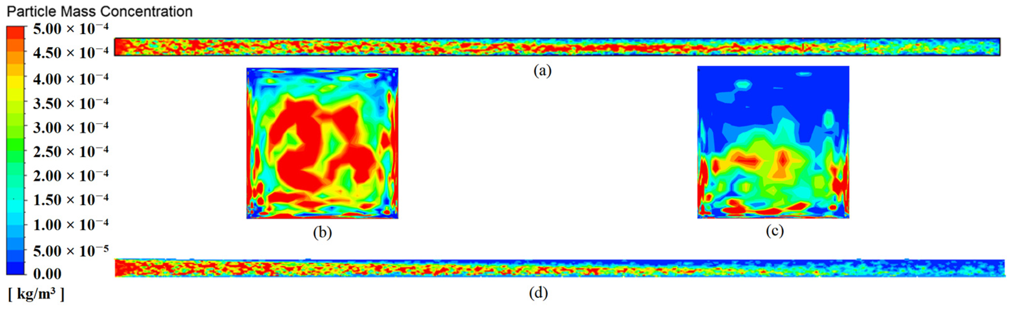
Figure 6 shows the particle-concentration-distribution cloud map obtained by simulating the particle deposition of 40 μm silica material in a pneumatic-conveying pipeline with a wind speed of 12 m/s by using the ellipsoid hypothesis and the sphere hypothesis, respectively. When the spherical hypothesis is adopted, the particles almost fill the pipe under the action of air flow, and there is a high concentration area near the pipe axis, as shown in Figure 6a. When the ellipsoid hypothesis is adopted, the particles show an increasingly obvious trend of gravitational and inertial settlement, and the area with high concentration of particles gradually deviates from the pipe axis along the pipe length direction and slopes down the pipe wall area, as shown in Figure 6d.
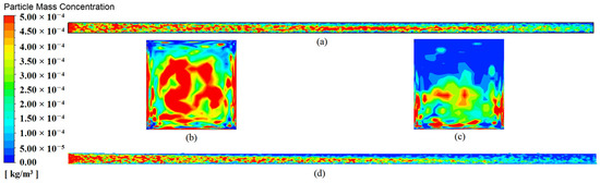
Figure 6.
Cloud map of particle-concentration distribution of gas pipeline at 12 m/s wind speed. (a) Sphericity hypothesis; (b) particle-concentration distribution at Y = 25 D cross-section of (a); (c) particle-concentration distribution at Y = 25 D cross-section of (d); (d) ellipsoid hypothesis.
In order to better observe the variation of the region with high particle concentration along the direction of the pipe diameter, vertical cross-section extraction was carried out at 15 m (Y = 25 D) along the direction of the pipe length in Figure 6a and Figure 6d, respectively. Among them, when the spherical hypothesis is adopted, the concentration distribution in the pipeline is mainly concentrated near the center of the section, and the high-concentration area is approximately rectangular. In the complex flow pattern near the wall, the particles are deviated by turbulence and the inertia of irregular fluid movement, showing a local high-concentration distribution, as shown in Figure 6b. When the ellipsoid hypothesis is adopted, the simulation results can better reflect the influence of gravity on the particles, and the particle concentration on the upper wall is significantly reduced. With the increase in particle size, the concentration-distribution area on both sides of the wall also tends to gradually decrease on the downward wall, and the high-concentration area moves downward from the center of the section, as shown in Figure 6c.
3.3.2. Particle Deposition of Simulation Results
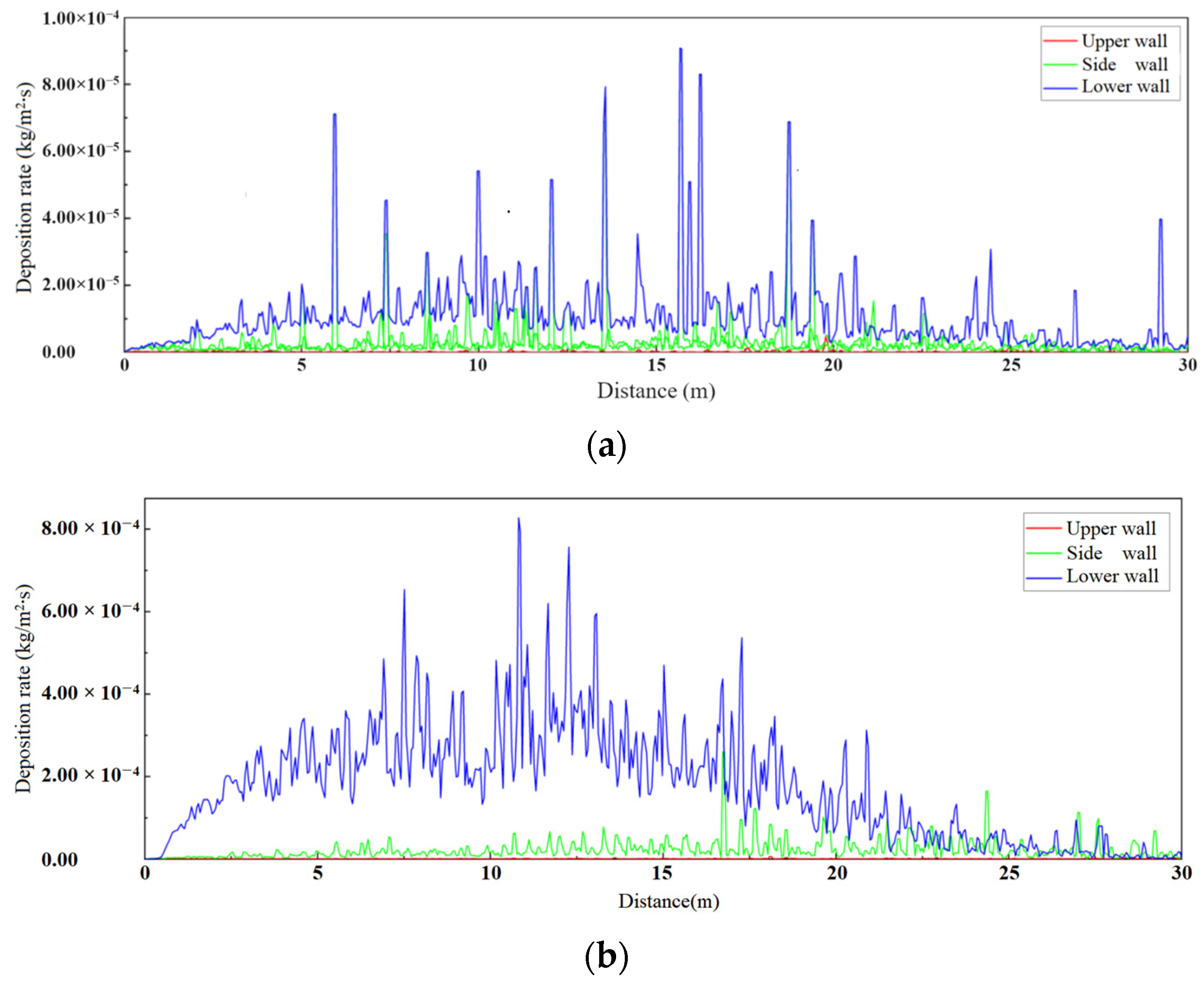
In order to directly characterize the influence of particle size on deposition location, the sediment mass per unit area recorded in UDM was extracted to quantify the deposition-location distribution of material particles under the two assumptions of spherical and ellipsoid; the results of particle-deposition efficiency on each wall of the gas pipeline were expanded along the length of the pipeline and are represented by a line graph, as shown in Figure 7.
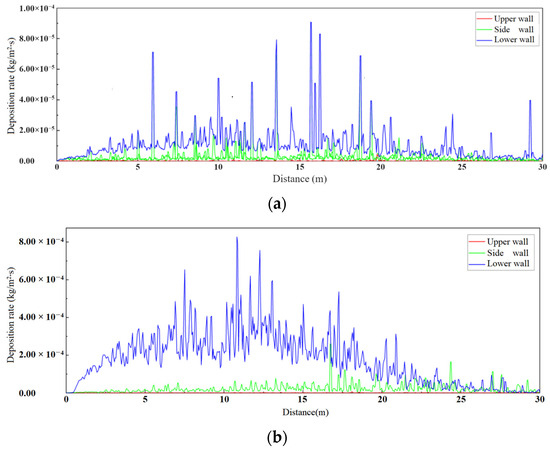
Figure 7.
Simulation results of particle deposition in gas pipelines at 12 m/s wind speed. (a) Sphericity hypothesis; (b) ellipsoid hypothesis.
Figure 7a shows the deposition efficiency of material particles on each wall of the pneumatic-conveying pipeline under the spherical assumption. The deposition distribution is mainly in the lower wall, reaching 1.57 × 10⁻³ kg/s. The average total deposition efficiency of the right wall and the left wall is 3.63 × 10⁻⁴ kg/s. They are much higher than 1.59 × 10⁻⁴ kg/s on the upper wall; the maximum-deposition interval is obvious, and the peak-deposition-efficiency interval is 13 D~28 D (the deposition efficiency in this area exceeds 52.04% of the total deposition efficiency). Under the ellipsoid assumption, the deposition efficiency of material particles on each wall of the pneumatic-conveying pipeline is shown in Figure 7b. The deposition distribution is also dominated by the lower wall, but the deposition efficiency reaches 2.01 × 10⁻³ kg/s. The average value of the total deposition efficiency of the right wall and the left wall decreased slightly, to 2.92 × 10⁻⁴ kg/s, while the upper wall remained basically the same, at 1.68 × 10⁻⁴ kg/s. The maximum deposition interval was also obvious, but the deposition efficiency was more concentrated and the peak interval changed. The area closer to the entrance is 5 D~18 D (the deposition efficiency of this area exceeds 73.79% of the total deposition efficiency). This is mainly because the deposition forms of 40 μm particles are mainly gravitational and inertial sedimentation, and the deposition distribution is significantly dominated by the lower-wall region, but the ellipsoid hypothesis is more sensitive to the impact of gravity and collision on material particles, which is consistent with the particle-concentration law described in Figure 6.
3.3.3. Particle-Deposition Morphology of Test Results
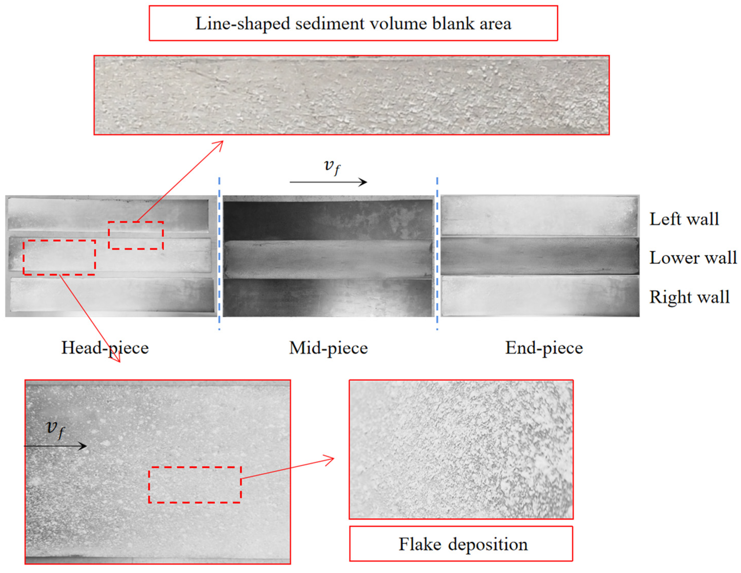
Through the particle-migration and deposition test under 12 m/s wind speed condition, the deposition conditions of a group of 30 D particle-sampling plates on the lower, left and right walls were obtained (because the hot-wire wind-speed sensor probe was installed on the upper wall of the particle transport pipeline, the sampling plate could not be arranged).
The overall deposition status of silicon dioxide (SiO2) samples was examined. As depicted in Figure 8, the overall particle-deposition morphology was streamlined in the same direction as the flow field. The deposition morphologies of the three wall surfaces were streamlined, and the particle-deposition amount was higher in the head-piece than in the end-piece. This is consistent with Figure 6d, for the numerical simulation. There is an obvious low-density area of particle deposition at the angle between the left wall and the lower wall of the head-piece. Figure 6c in the simulation also provides the corresponding simulation. Moreover, the deposition phenomenon of Flak-deposition is presented, and this phenomenon is in accordance with the numerical-simulation results using the ellipsoid hypothesis in Section 3.3.2.
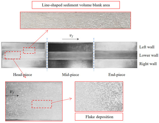
Figure 8.
Experimental collection of particle transport at 12 m/s wind speed.
3.3.4. Comparison of Simulation Results and Test Results
In order to measure the difference between the simulation results of particle migration and deposition and the experimental-simulation results, the sediment particles on the lower wall of the sample simulated by the experiment were collected and weighed, and the simulation results under the spherical hypothesis and the ellipsoid hypothesis were compared (comparison range: 0 D ≤ L ≤ 30 D), as shown in Figure 9. MR is defined as the ratio of the mass of the bottom deposited particles per-unit-length D to the total mass of all the bottom deposited particles, MRs-S is the simulation result of the spherical hypothesis, MRs-E is the simulation result of the spherical hypothesis, and MRt is the experimental-simulation result.
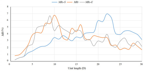
Figure 9.
Scatter plot comparing simulation results and experimental results of lower-wall particle deposition for sample.
It can be seen that the particle-deposition efficiency curve under both assumptions can reflect certain deposition laws. Among these, the spherical hypothesis assumes that the peak range of deposition efficiency is (13 D~28 D), the ellipsoidal hypothesis assumes that the peak range of deposition efficiency is (5 D~18 D), and the peak range of particle deposition efficiency in the experimental simulation is (6 D~16 D); it can be seen that the simulation results under the ellipsoid hypothesis are closer to the experimental-simulation results. The accuracy of the pipeline particle-deposit model is based on the ellipsoid hypothesis, and its superiority in engineering applications are verified.
4. Conclusions
- (1)
- The established hypothetical ellipsoidal particle-deposition model provides a fast algorithm for the deposition efficiency and distribution of material transportation under working conditions, which can be brought into the drag-force correction coefficient K. This can show the deposition characteristics of material particles during pneumatic transportation in detail, and verify the effectiveness and effectiveness of the model based on particle-migration- and deposition-simulation experiments, to determine the accuracy of the algorithm.
- (2)
- Based on the proposed ellipsoid hypothesis, the numerical simulation of the pneumatic transportation pipeline of SiO2 particles is carried out, and the peak value of the material particle-deposition efficiency is obtained from (5 D~18 D). The experimental simulation of SiO2 on the particle-transport- and deposition-simulation platform is carried out, and the peak value range of the sample particle-deposition efficiency is obtained from (6 D~16 D).
- (3)
- The proposed algorithm for rapid deposition of material particles under the ellipsoid hypothesis is based on the drag-force correction-coefficient table given by the typical ellipsoid parameters. It still has a lot of room for improvement in the research of expanding the range of ellipsoid parameters and refining the parameter categories.
- (4)
- In the future, based on this model, the deposition laws of mixed materials and particle-size composite materials can be explored in the context of different pneumatic conveying, and the recommended indicators of pneumatic-conveying technology for mixed materials can be given. At the same time, the effects of pneumatic-conveying pipe length, pipe type, and pipe-body material on material particle-deposition characteristics can be further studied through simulation and experiments, and suggestions for the optimization of standard pneumatic-conveying pipelines in different environments can be given.
Author Contributions
Conceptualization, C.N. and Z.Z.; methodology, C.N.; software, C.N. and J.Q.; validation, C.N., X.Y. and Z.Z.; formal analysis, C.N.; investigation, J.Q.; resources, Z.Z.; data curation, C.N.; writing—original draft preparation, C.N.; writing—review and editing, C.N. and J.Q.; visualization, X.Y.; supervision, J.Q.; project administration, J.Q.; funding acquisition, Z.Z. All authors have read and agreed to the published version of the manuscript.
Funding
This research received no external funding.
Data Availability Statement
Laboratory data will not be uploaded to the database for the time being. If necessary, please email the corresponding author for consultation.
Conflicts of Interest
The authors declare no conflicts of interest.
References
- Du, J.; Hu, G.M.; Fang, Z.Q.; Wang, J. Simulation of dilute pneumatic conveying with different types of bends by CFD-DEM. In Proceedings of the 27th Symposium on Hydraulic Machinery and Systems, Montreal, QC, Canada, 22–26 September 2014; IAHR: The Hague, The Netherlands, 2014. [Google Scholar]
- Klinzing, G.E. A review of pneumatic conveying status, advances and projections. Powder Technol. 2018, 333, 78–90. [Google Scholar] [CrossRef]
- Ebrahimi, M.; Crapper, M.; Ooi, J.Y. Experimental and simulation studies of dilute horizontal pneumatic conveying. Particul. Sci. Technol. 2014, 32, 206–213. [Google Scholar] [CrossRef]
- Ebrahimi, M.; Crapper, M. CFD-DEM simulation of turbulence modulation in horizontal pneumatic conveying. Particuology 2016, 31, 15–24. [Google Scholar] [CrossRef]
- Bhattarai, S.; Oh, J.H.; Euh, S.H.; Kim, D.H.; Yu, L. Simulation study for pneumatic conveying drying of sawdust for pellet production. Dry Technol. 2014, 32, 1142–1156. [Google Scholar] [CrossRef]
- Zhou, J.; Shangguan, L.; Gao, K.; Wang, Y.; Hao, Y. Numerical study of slug characteristics for coarse particle dense phase pneumatic conveying. Powder Technol. 2021, 392, 438–447. [Google Scholar] [CrossRef]
- de Almeida, E.; Spogis, N.; Taranto, O.P.; Silva, M.A. Theoretical study of pneumatic separation of sugarcane bagasse particle. Biomass Bioenerg. 2019, 127, 105256. [Google Scholar] [CrossRef]
- Xu, D.; Li, Y.; Xu, X.; Zhang, Y.; Yang, L. Numerical study of wheat particle flow characteristics in a horizontal curved pipe. Processes 2024, 12, 900. [Google Scholar] [CrossRef]
- Guzman, L.; Chen, Y.; Landry, H. Coupled CFD-DEM simulation of seed flow in an air seeder distributor tube. Processes 2020, 8, 1597. [Google Scholar] [CrossRef]
- Guzman, L.; Chen, Y.; Landry, H. Coupled CFD-DEM Simulation of seed flow in horizontal-vertical tube transition. Processes 2023, 11, 909. [Google Scholar] [CrossRef]
- Zhou, J.W.; Yan, X.Y.; Zheng, Z.B.; Wang, Q.H.; Shangguan, L.J. Research status and prospect of key installations and flow characteristics of pneumatic conveying. Chin. J. Process Eng. 2023, 23, 649–661. [Google Scholar]
- Cui, Z.W.; Wang, Z.; Jiang, X.Y.; Zhao, L.H. Numerical study of non-spherical particle-laden flows. Adv. Mech. 2022, 52, 623–672. [Google Scholar]
- Lee, L.Y.; Quek, T.Y.; Deng, R.; Ray, M.B.; Wang, C.H. Pneumatic transport of granular materials through a bend. Chem. Eng. Sci. 2004, 59, 4637–4651. [Google Scholar] [CrossRef]
- Brooke, J.W.; Hanratty, T.J.; McLaughlin, J.B. Free-flight mixing and deposition of aerosols. Phys. Fluids 1994, 6, 3404–3415. [Google Scholar] [CrossRef]
- Chen, M.; McLaughlin, J.B. A New Correlation for the Aerosol Deposition Rate in Vertical Ducts. J. Colloid Interface Sci. 1995, 1692, 437–455. [Google Scholar] [CrossRef]
- Wang, Q.; Squires, K.D. Large Eddy Simulation of Particle2laden Turbulent Channel Flow. Phys. Fluids 1996, 8, 1207–1223. [Google Scholar] [CrossRef]
- Sun, Z.; Wang, Y.; Yuan, C. Influence of Oil Deposition on the Measurement Accuracy of a Calorimetric Flow Sensor. Measurement 2021, 185, 110052. [Google Scholar] [CrossRef]
- Liu, H.; Zhang, L.; Chen, T.; Wang, S.; Han, Z.; Wu, S. Experimental Study on the Fluidization Behaviors of the Superfine Particles. Chem. Eng. J. 2015, 262, 579–587. [Google Scholar] [CrossRef]
- Shi, H.X. Experimental Research of Flow Structure in a Gas-solid Circulating Fluidized Bed Riser by PIV. J. Hydrodyn. Ser. B 2007, 19, 712–719. [Google Scholar] [CrossRef]
- Yan, F.; Rinoshika, A.; Zhu, R.; Tang, W.X. The effect of oscillating flow on a horizontal dilute-phase pneumatic conveying. Particul. Sci. Technol. 2016, 35, 699–706. [Google Scholar] [CrossRef]
- Kotzur, B.A.; Berrr, R.; Zigan, S.; García-Triñanes, P.; Bradley, M.S.A. Particle attrition mechanisms, their characterisation, and application to horizontal lean phase pneumatic conveying systems: A review. Powder Technol. 2018, 334, 76–105. [Google Scholar] [CrossRef]
- Olaleye, A.K.; Shardt, O.; Walker, G.M.; Van den Akker, H.E.A. Pneumatic Conveying of Cohesive Dairy Powder: Experiments and CFD-DEM Simulations. Powder Technol. 2019, 357, 193–213. [Google Scholar] [CrossRef]

Disclaimer/Publisher’s Note: The statements, opinions and data contained in all publications are solely those of the individual author(s) and contributor(s) and not of MDPI and/or the editor(s). MDPI and/or the editor(s) disclaim responsibility for any injury to people or property resulting from any ideas, methods, instructions or products referred to in the content. |
© 2024 by the authors. Licensee MDPI, Basel, Switzerland. This article is an open access article distributed under the terms and conditions of the Creative Commons Attribution (CC BY) license (https://creativecommons.org/licenses/by/4.0/).