Numerical Simulation of Internal Flow Field in Optimization Model of Gas–Liquid Mixing Device

Abstract

This article studies the influence of structural parameters of the optimization model for the gas–liquid mixing device of a fire truck (compressed air foam lift fire truck, model JP21/G2, made in China) on the liquid phase volume fraction, static pressure, velocity streamline, and the influence of smaller flow rates on the mixing effect. By using the computational fluid dynamics (CFD) software FLUENT 2021 R2, numerical simulations were conducted on the fluid domain model of the gas–liquid mixing device of the JP21/G2 fire truck. The changes in the mixing effect time dimension, liquid phase volume fraction, static pressure, and velocity streamline inside the gas–liquid mixing device were obtained. The optimal mixer structure combination in practical applications was inferred through orthogonal experiments, and the influence of flow rate on the optimal pipe diameter and shortest mixing distance was obtained through variable flow rate simulation experiments. The numerical simulation results show that the presence of bent pipes in the JP21/G2 real vehicle model hinders the gas–liquid mixing process. A straight pipe section of at least 8 m was added after the bent pipe to ensure the mixing effect. The optimal parameter combination for orthogonal experiments had an accurate value of 50°-50°-220 mm. Under the same pipe diameter, using a larger flow rate can achieve better mixing effects.

1. Introduction

Fire is an essential part of daily life, but due to people’s incorrect use of fire, it can lead to fires, causing losses to our life and property safety, especially residential fires, which account for 25.6% of total fire accidents and cause a large number of casualties [1,2,3,4,5]. Moreover, with the rapid development of China’s economy and the acceleration of urbanization, a large number of people are migrating to cities, resulting in an increasing urbanization rate and increasing fire hazards in cities [6,7,8,9,10]. There are also forest fires that are difficult to control. There are many forested areas in China, and there are also serious fire hazards [11,12,13,14,15,16]. How to effectively extinguish various types of fires when they occur is a problem that we need to study.

People have also studied fire extinguishing methods corresponding to different types and ignition methods of fires. Chen et al. [17] used a self-built pneumatic sandblasting fire extinguishing experimental platform to study the distribution of sand particles, fire extinguishing efficiency, and fire extinguishing mechanism. They found that sand can effectively accumulate at a distance of 1.5–2.34 m from the water outlet. The use of pneumatic sandblasting fire extinguishers can greatly shorten the fire extinguishing time. Therefore, it is recommended to use sand in pneumatic fire extinguishers to improve the early fire extinguishing performance of forest fires. Wang et al. [18] designed a novel composite additive and water mist-compatible fire extinguishing method and studied the fire extinguishing ability and influence of composite additives containing water mist on lithium-ion battery fires. The study found that physical and chemical additives have important physical and chemical effects on fire extinguishing, which are more effective than pure water mist. Sheng et al. [19], based on long-chain fluorinated surfactant and short-chain fluorinated surfactant, and based on the mixture of silicone surfactant and foam stabilizer, prepared a fluorine-free foam. This research can guide the development of environmentally friendly fire foam. The study by Aydin et al. [20] demonstrates the collaborative use of drones and remote sensing technology as supplements to traditional firefighting methods, showcasing the construction of heavy payload drones and introducing the development progress of fire suppression ball devices that can be hung on drones. Deng et al. [21] conducted a compressed nitrogen spray test and a compressed air spray test, respectively, and discussed the feasibility of using compressed air to replace compressed nitrogen in composite jets. The results showed that there was little difference between the two gases in extinguishing pool fire, indicating that it was feasible to use compressed air as the driving gas of composite jet in the process of extinguishing fire. In addition, effective fire extinguishing methods for specific environments still need to be studied.

Researchers have conducted several studies on bubbling in mixers. Yuan et al. [22] conducted experimental and numerical studies on the flow resistance and bubble transport in a spiral static mixer and found that the variation of bubble size decreases with the change of Reynolds number. Jia et al. [23] demonstrated a unique method of using bubbles to promote the mixing of large amounts of solutions, which has potential applications in microfluidics, rapid medical analysis, and biochemical synthesis. Hashemi et al. [24] studied the effect of flow hydrodynamics generated by impellers on bubble size, demonstrating the effect of velocity ratio on bubble rupture through anchor blades. Dietrich et al. [25] studied the shape, size, and formation mechanism of bubbles, and the results showed that the formation of bubbles, especially their size, depends on the geometric shape of the mixing part between the two phases. The application of research on bubbling in mixers to firefighting equipment can improve firefighting efficiency and reduce the damage caused by fires to personnel and property. However, it is worth further studying which liquid and gas phases should be mixed and under what conditions to achieve better fire extinguishing effects.

The gas–liquid mixing device, as the core component of fire trucks, has been studied by some people. Zhou et al. [26] designed and established a mixing device that combines the advantages of jet and mixing dispersion. The suction performance of the device is significantly improved, which is conducive to the mixing of gas and liquid phases. Liu et al. [27] investigated the effects of working conditions and structural configuration of a cyclone head on gas–liquid characteristics (volume mass transfer coefficient, gas resistance, and bubble dispersion). The research results showed that gas–liquid mass transfer performance is influenced by structural parameters such as blade angle, blade curvature, and stator bottom opening. Amiri et al. [28] proposed the application of jet fluid as a mixer in gas–liquid systems. By installing experimental devices, the mixing behavior of the liquid phase was further studied. Gas flow and jet countercurrent were injected into the mixing container to investigate the effects of jet injection, conductivity probe position, aeration rate, and jet Reynolds number on mixing time. Hou et al. [29] studied a novel high-throughput gas–liquid mixer with a tree-like structure using the method of absorbing pure carbon dioxide. The volume mass transfer coefficient, interface area, liquid surface mass transfer coefficient, and pressure drop of the micromixer were determined under different configurations and operating conditions. Khopkar et al. [30] studied the gas–liquid flow generated by a turbine with three lower pump inclined blades, and their computational model and results help explain the influence of local flow patterns on the mixing process. The impact of mixers with different structures on gas–liquid mixing varies. Based on a comprehensive understanding of the structural design and working principle of the gas–liquid mixing device, we optimized it and conducted simulations under certain parameter conditions to achieve better mixing effects.

In summary, this article uses the CFD simulation method to numerically simulate the fluid domain model of the JP21/G2 fire truck gas–liquid mixing device and studies the influence of structural parameters of the optimized model of the JP21/G2 fire truck gas–liquid mixing device on the liquid phase volume fraction, static pressure, and velocity streamline. By conducting orthogonal experiments, the coefficient of variation (COV) value of the uniformity coefficient can be obtained, and comparing the COV value of the uniformity coefficient can lead to the optimal combination of mixer structures in practical applications. Based on the original simulation conditions, the flow rate of the foam liquid can be changed to obtain the change rule with the best pipe diameter and the shortest mixing distance.

2. Methodology

2.1. Numerical Methods

The CFD method has been widely recognized as an efficient method for studying the motion behavior of gas–liquid two-phase flow [31,32,33]. This study uses the Euler–Lagrange coupling method to calculate the mixing mechanism of the internal flow field in the optimization model of gas–liquid mixing devices.

The Euler–Lagrange model solves the mass and momentum conservation equations of the liquid phase (liquid) in the Euler coordinate system to obtain the liquid flow field. In the Lagrange coordinate system, by solving the force balance equation of dispersed phase particles or bubbles, the motion trajectory of the discrete phase is obtained [34,35,36,37]. The Navier–Stokes equations and the independent momentum equation control the motion of continuous and discrete phases, respectively. A turbulence model was established based on the renormalization group (RNG) $k-\epsilon$ model [38,39,40], which can effectively simulate strongly coupled isotropic fluids [41]. The continuity equation is represented as follows:

$${\displaystyle \frac{\partial }{\partial t}}({\rho }_m)+\nabla \cdot ({\rho }_m{\overline{\upsilon }}_m)=0$$

(1)

with

$${\overline{\upsilon }}_m={\displaystyle \frac{{\displaystyle \sum _{k=1}^n{\phi }_k{\rho }_k{\overline{\upsilon }}_k}}{{\rho }_m}}$$

(2)

$${\rho }_m={\displaystyle \sum _{k=1}^n{\phi }_k}{\rho }_k$$

(3)

where $k$ is the number of fluid phases in the model, ${\rho }_k$ is the density of $k$, ${\phi }_k$ is the volume fraction of $k$, ${\overline{\upsilon }}_k$ is the average velocity of $k$, and $\nabla \cdot ({\rho }_m{\overline{\upsilon }}_m)$ is the mass flux of the surface area of the control body.

The momentum equation is expressed as follows:

$${\displaystyle \frac{\partial }{\partial t}}({\rho }_m{\overline{\upsilon }}_m)+\nabla \cdot ({\rho }_m{\overline{\upsilon }}_m{ }^2)=-\nabla P+\nabla \cdot [{\mu }_m(\nabla {\overline{\upsilon }}_m+\nabla {\overline{\upsilon }}_m{ }^T)]+\rho mg+f$$

(4)

where ${\mu }_m$ is the viscosity coefficient of the mixture, $g$ is the gravitational acceleration, and $f$ is the volumetric force.

For gas–liquid two-phase flow, surface tension has a significant impact on fluid flow and cannot be ignored [42,43,44]. The calculation of surface tension can be written as follows:

$$F={\displaystyle \frac{2\rho \sigma {\kappa }_G\nabla \alpha }{{\rho }_L+{\rho }_G}}$$

(5)

where $\rho$ is the flow density, ${\kappa }_G$ is the curvature of the liquid–gas phase interface, and $\sigma$ is the surface tension. Among them, ${\kappa }_G$ can be calculated as follows:

$${\kappa }_G=\nabla \widehat{n}=\nabla {\displaystyle \frac{\overrightarrow{n}}{\left|\overrightarrow{n}\right|}}$$

(6)

$$\widehat{n}=\widehat{n}\cos \theta +\sqrt{1-\widehat{n}{ \sin }^2 \theta }$$

(7)

where $\widehat{n}$ is the size of the unit normal vector related to the contact angle $\theta$.

The parameters widely used to evaluate the mixing effect currently include relative standard deviation, coefficient of variation, residence time distribution, tensile value, shear rate, etc. In this study, the coefficient of uniformity COV value was used as one of the indicators to evaluate the mixing effect [45].

The definition of the coefficient of uniformity COV value is determined by adding a certain amount of dispersed phase at the inlet, dividing the entire region into N equally sized regions on the outlet cross-section (this study is divided into 7 regions, as shown in Figure 1), and using the volume fraction of dispersed phase in the i-th region, ${\phi }_i$ represents the following:

$$COV={\displaystyle \frac{\sigma }{\overline{\phi }}}={\displaystyle \frac{\sqrt{\frac{1}{N}{\displaystyle \sum _{i=1}^n({\phi }_i-\overline{\phi })}}}{\frac{1}{N}{\displaystyle \sum _{i=1}^n{\phi }_i}}}$$

(8)

where ${\phi }_i$ represents the volume fraction of the dispersed phase in the i-th region and $\overline{\phi }$ represents the average volume fraction of the dispersed phase across the entire cross-section.

According to the mathematical definition of the formula, the smaller the COV value, the more uniform the mixing. When the COV value in industry is less than 0.05, it is considered that the mixture is uniform.

Table 1. Operating condition parameters table.

	Foam Agent	Compressed Air
Flow Q (L/min)	10,000	50,000
Pressure P (MPa)	1	1.1
Hydraulic diameter D (mm)	250	60
Density ρ (kg/m3)	1010	13.072
Dynamic viscosity μ (kg/(m·s))	0.0187	1.82 $\times$ 10−5
Speed v (m/s)	3.397	98.294

shows the setting of operating parameters. The turbulence model adopts the mixture two-phase flow model. The main phase is the liquid phase (foam agent), and the secondary phase is the gas phase (compressed air). The realizable $k-\epsilon$ discrete format is used. The velocity inlet is used as the boundary inlet, and the pressure outlet is used as the outlet boundary condition. The pressure, momentum, and turbulent kinetic energy are discretized using the quick method, and the simulation time step is 0.001 s.

Since the mass concentration of foam in Class A foam concentrate is small, the water phase is the main phase of the foam agent, and the secondary phase is air. Considering the influence of gravity on the mixing effect, set the gravity acceleration to 9.81 m/s and the direction to the negative z-axis. The liquid inlet of the model adopts the velocity inlet boundary, and its value changes with the change of foam liquid inlet pipe diameter; the gas phase inlet adopts a mass flow inlet; the outlet adopts a pressure outlet boundary; and the outlet pressure is set to atmospheric pressure.

To evaluate the mixing effect, four evaluation indicators were used: liquid phase volume fraction contour, pressure drop before and after the mixing chamber, COV value of liquid phase volume fraction uniformity coefficient, and liquid phase velocity streamline. The evaluation criteria are shown in

Table 2. Data post-processing evaluation indicators.

Evaluating Indicator	Evaluation Criterion
Liquid phase volume fraction contour	The more vortices there are, the more thorough the mixing of the two phases is; the more uniform the size of the vortex, the better
Pressure drop before and after mixing chamber	The smaller the pressure drop value, the less energy consumption it indicates
Uniformity coefficient COV value	The smaller the COV value, the better the fluid uniformity and the value drops to 0.05, reaching the industrial standard
Liquid phase velocity streamline	The sparser and more uniform the streamline distribution, the higher the mixing stability

.

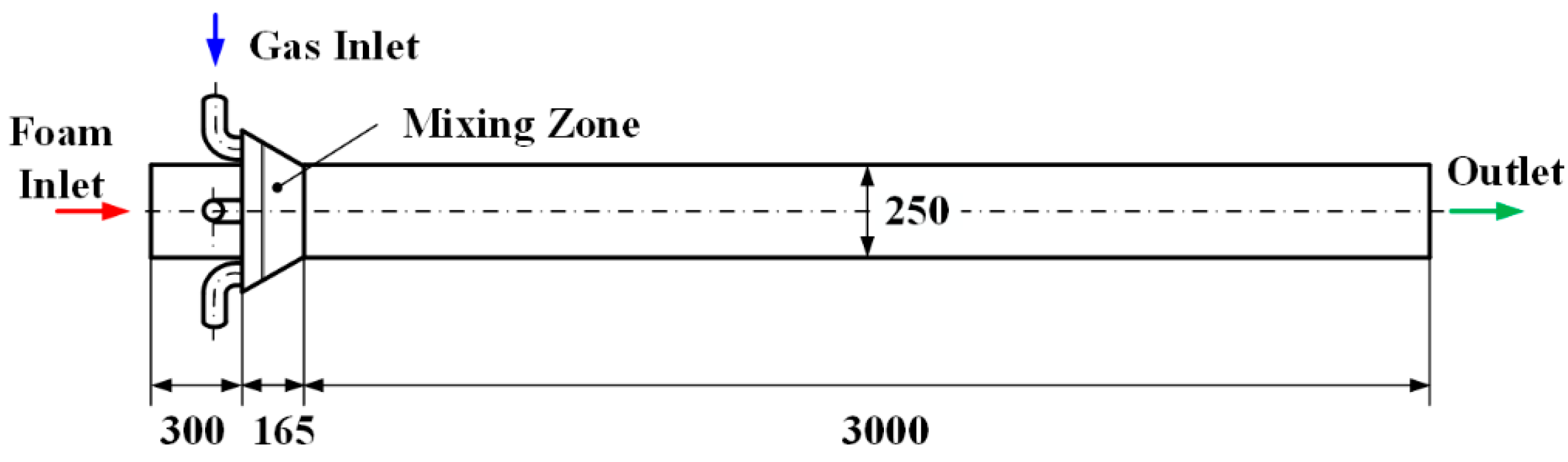
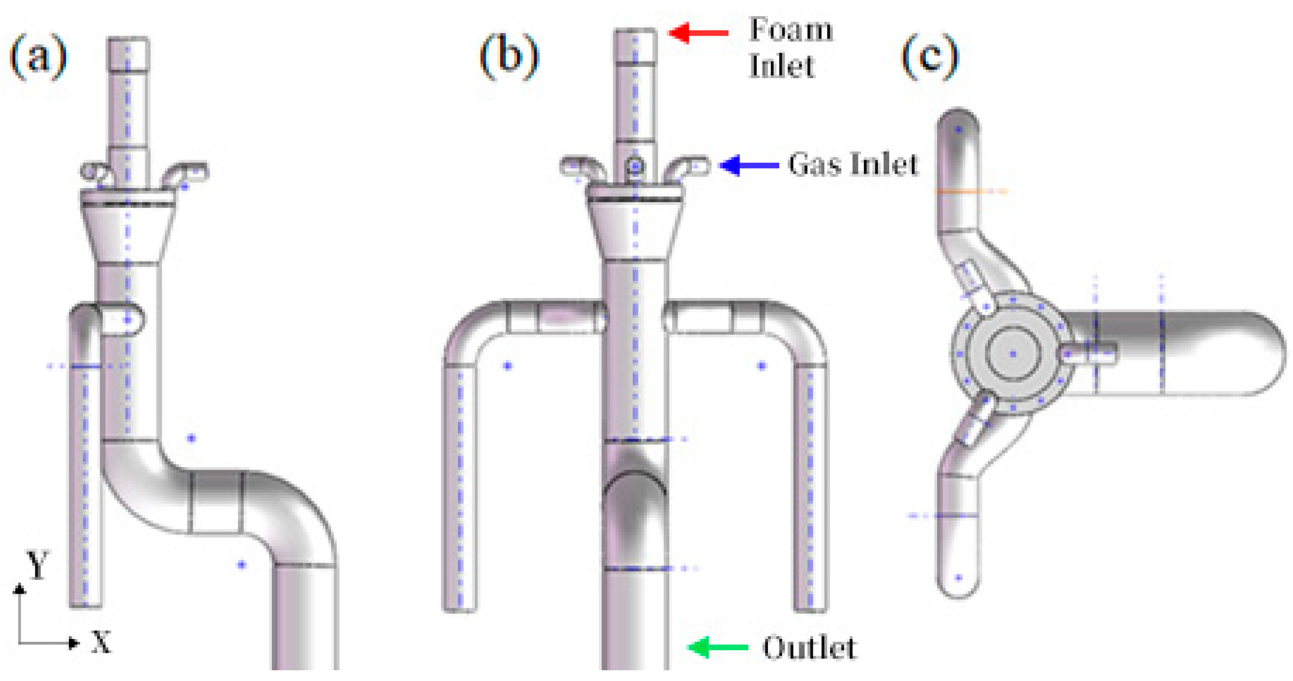
2.2. Experimental Setup

The geometric model of the mixer is shown in Figure 2, with geometric structural parameters of 60° cone angle, 60° inlet inclination angle, and 250 mm diameter pipeline. The mixer cone angle θ, inlet inclination angle β, and pipe diameter D are shown in Figure 3. The gas–liquid mixing device consists of four fluid domains: gas phase inlet (Gas Inlet), liquid phase inlet (Foam Inlet), mixing chamber, and mixing chamber outlet. The foam liquid and compressed air enter the conical mixing chamber through the inlet for mixing, and then the mixed liquid flows to the outlet along the outlet pipeline. The liquid phase inlet has a diameter of 250 mm; the gas phase inlet has a total of three, with a diameter of 60 mm; and the outlet pipeline has a diameter of 250 mm.

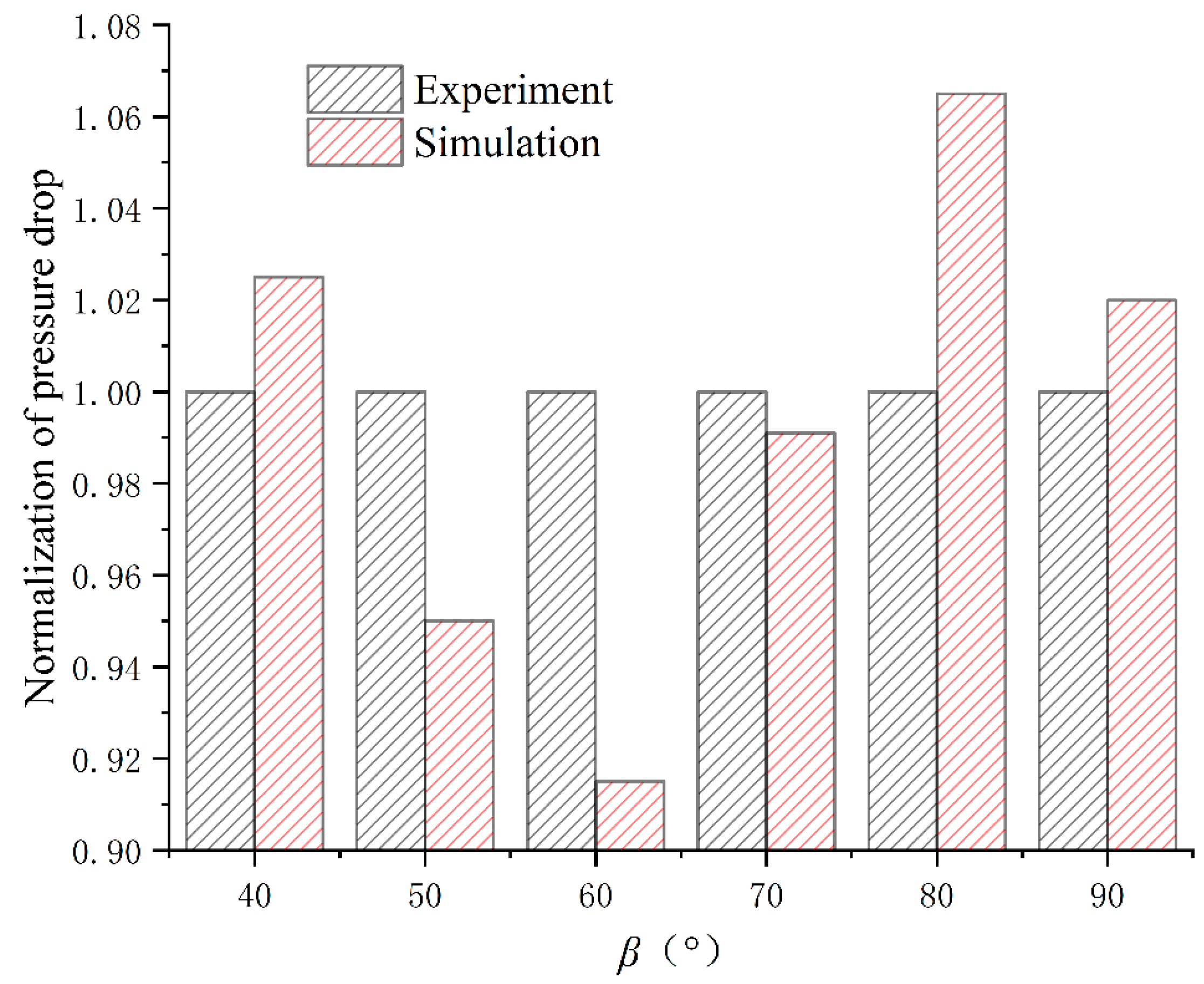
2.3. Simulation Model Verification

The reliability of numerical simulation needs to be verified through experiments or theoretical models. The mesh elements are set to twice the particle size to ensure the accuracy of the void ratio, which is 9 mm. The study on mesh independence is shown in Figure 4. The pressure drop in the flow field is one of the most important parameters in gas–liquid mixing systems. Based on on-site experiments, this article uses the normalized pressure drop between 50 mm before and after the mixing chamber of the gas–liquid mixing device as a comparative indicator to describe the impact of different tilt angle mixers on energy loss. The results are shown in Figure 5. The normalized pressure drop in the figure is defined as the ratio of each pressure drop value to the average pressure drop value.

From Figure 5, it can be seen that there is a slight difference between the numerical simulation results and the experimental results. This phenomenon is caused by the following reasons: on the one hand, there is a large eddy current in the gas–liquid phase inside the mixer, and there is a large random error in the interaction between the two phases, so there may be some differences; on the other hand, the length of the pipeline used in the experiment and simulation is inconsistent, and to prevent grid distortion, the simulation model is slightly simplified compared to the actual model, resulting in differences in results. However, overall, the numerical calculation results are consistent with the experimental results, especially when the inclination angle is 70°. The numerical calculation and experimental results are in good agreement, so the numerical model used has high reliability.

3. Results and Discussion

3.1. Numerical Simulation of the JP21/G2 Fire Truck

Based on the actual connection size of the gas–liquid mixing device of the JP21/G2 fire truck, a simulation model is established, and numerical simulation is carried out as follows:

The fluid domain model of the JP21/G2 fire truck is shown in Figure 6:

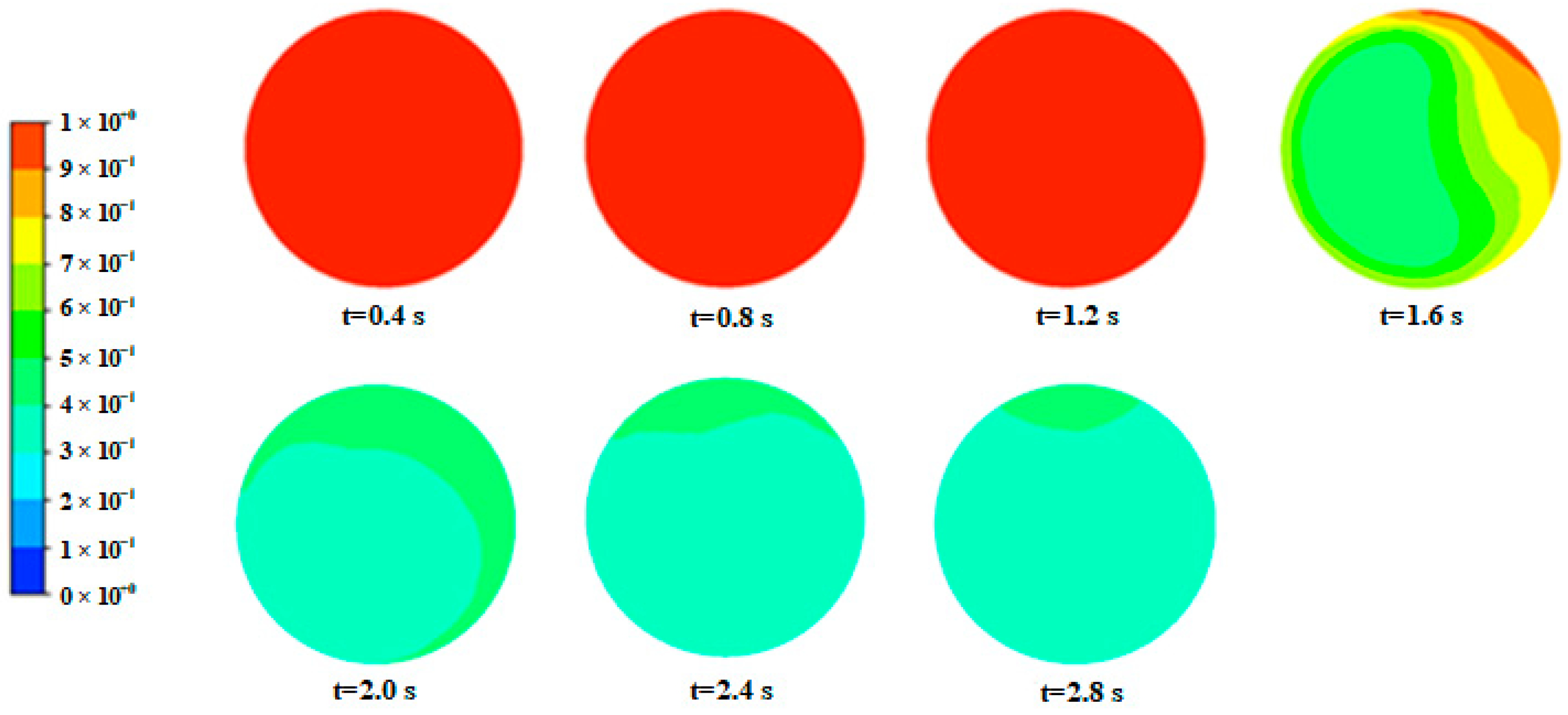
3.1.1. Changes in the Time Dimension of Mixing Effects

The simulation conditions set in this section are as follows: the liquid phase flow is 10,000 L/min, the gas phase flow is 50,000 L/min, the gas phase inlet pressure is 1.0 MPa, the liquid phase inlet pressure is 1.1 MPa, the cone angle is 60°, the foam liquid inlet pipe diameter is 250 mm, and the gas phase inlet is 60 mm. To explore when the JP21/G2 mixer with a length of 10 m at the rear end of the mixing chamber can reach a uniform mixing state, during simulation initialization, it is assumed that the foam solution fills the entire fluid domain, and then compressed air is injected into it. The volume fraction of the liquid phase at the outlet of the mixer is monitored every 0.4 s, and the comparison contour is shown in Figure 7. It can be seen from the figure that before the mixing time is 1.2 s, the compressed air does not flow to the outlet of the mixer, so the contour of the liquid phase volume fraction maintains the state that is full of foam during initialization; when mixing for up to 1.6 s, the gas phase has already occupied a certain volume fraction at the outlet, but the mixing state is poor, manifested by a large color gradient; when the mixing time reaches 2.0 s, the mixing state is already ideal, manifested as a small color difference in the cloud image; the difference in contours within the range of 2.0~2.8 s during mixing is small, indicating that the two-phase mixing approximately reaches a stable state at 2.0 s.

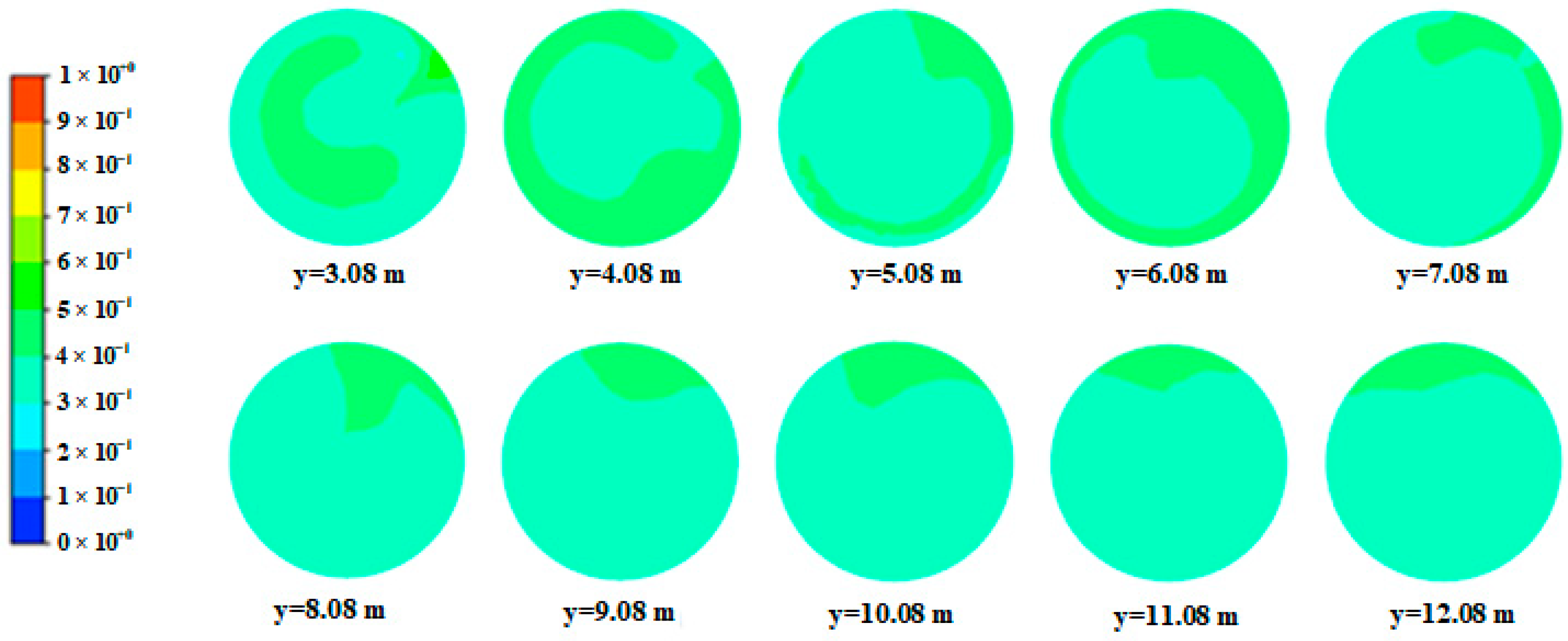
3.1.2. Variation Law of Liquid Phase Volume Fraction

The main pipeline at the rear end of the mixing chamber with a mixing time of 2.4 s is taken as the research object, and a cross-section is taken every 1 m forward of the outlet of the self-mixer as monitoring points. The contour of the change in liquid phase volume fraction is shown in Figure 8. From the graph, it can be observed that as the mixing distance increases, the uniformity of liquid phase distribution gradually increases; the position where the volume fraction gradient is generated gradually moves from the center to the pipe wall, and the gradient size and distribution range gradually decrease; the proportion of liquid phase at the center of the pipeline is smaller than that at the pipe wall.

Figure 9 shows the variation of the coefficient of uniformity COV value with mixing distance (from the moment liquid and gas come into contact in the mixing chamber until the mixture is discharged from the outlet). From the graph, it can be seen that the variation pattern of COV value is as follows: when the mixing distance is 1–5 m, the COV value gradually decreases, indicating that the degree of mixing gradually deepens; a turning point appears at 5 m, and the COV value increases at 5–7 m due to flow pulsation caused by high turbulence energy in this section of the pipeline; subsequently, as turbulent pulsation dissipates, the COV value gradually decreases. Due to the standard for uniform mixing in the industry being a COV value of 0.05, it can be considered that the gas–liquid mixture has reached a uniform state at a mixing distance of 8 m.

Figure 10 shows the contour of the change in liquid phase volume fraction before and after the mixing chamber. From the figure, it can be seen that the volume fraction of the liquid phase is relatively uniform at the bend, indicating that the presence of bending has a positive impact on mixing, and bending makes the mixing more uniform; the liquid phase is affected by gravity and exhibits uneven distribution in the pipeline, concentrated on one side along the direction of gravity; due to the high fluid velocity and turbulent kinetic energy, a certain amount of turbulence will be generated.

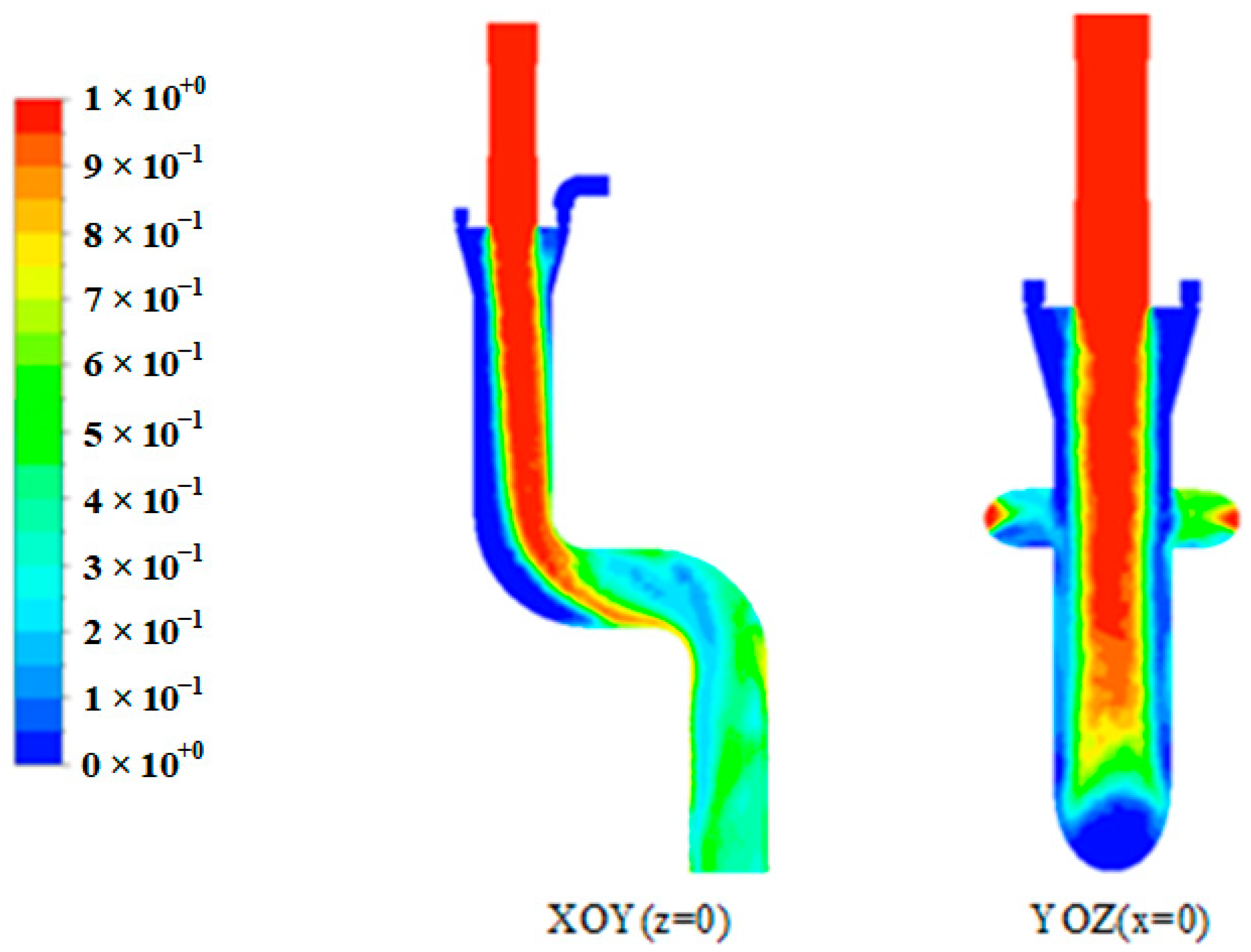
3.1.3. Static Pressure Variation Pattern

Figure 11 shows the contour of static pressure changes before and after the mixing chamber. It can be seen that there is a static pressure loss at the bend, which is caused by a sharp change in the flow velocity and direction of the fluid when passing through the bend. The fluid does not participate in active flow in this area, but continuously swirls, causing additional friction and collisions between particles, resulting in significant energy loss; when the diameter of the pipeline at the front end of the mixing chamber changes, energy loss can also be caused. The reason is that the energy of pressure and resistance always needs to be conserved. The change in pipeline diameter will lead to an increase in resistance, which can only be compensated for by reducing static pressure, thereby increasing energy loss; when passing through the mixing chamber, there will also be a certain amount of energy loss, mainly due to changes in pipe diameter, two-phase collisions, and increased flow velocity leading to energy loss along the way.

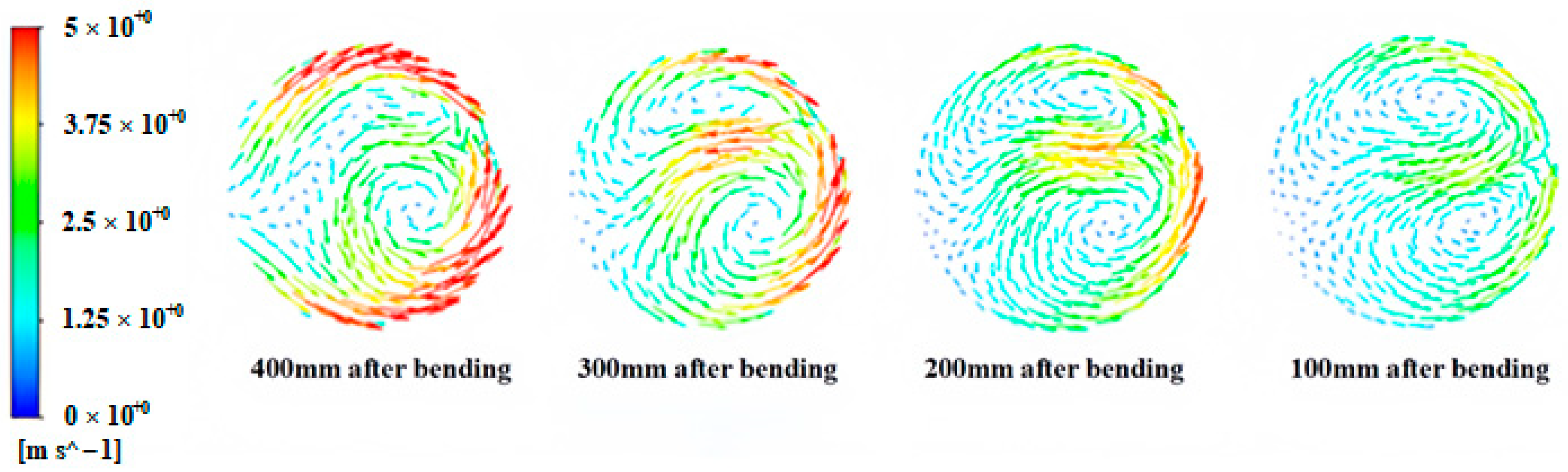
3.1.4. Speed Streamline

As shown in Figure 12 and Figure 13, the velocity streamline of the pipeline before and after the bend is compared. From the figure, it can be seen that at the front end of the bend, as the mixing distance increases, the velocity streamline gradually becomes uniform. The vortices in the streamline diagram gradually disappear, and the velocity gradually increases, indicating that the mixing uniformity is getting better and better; at the back end of the bend, new vortices are generated, turbulence intensifies, and the speed gradually decreases, indicating that the presence of the bend is not conducive to uniform mixing; the velocity at the pipe wall is greater than that in the central area, regardless of the location.

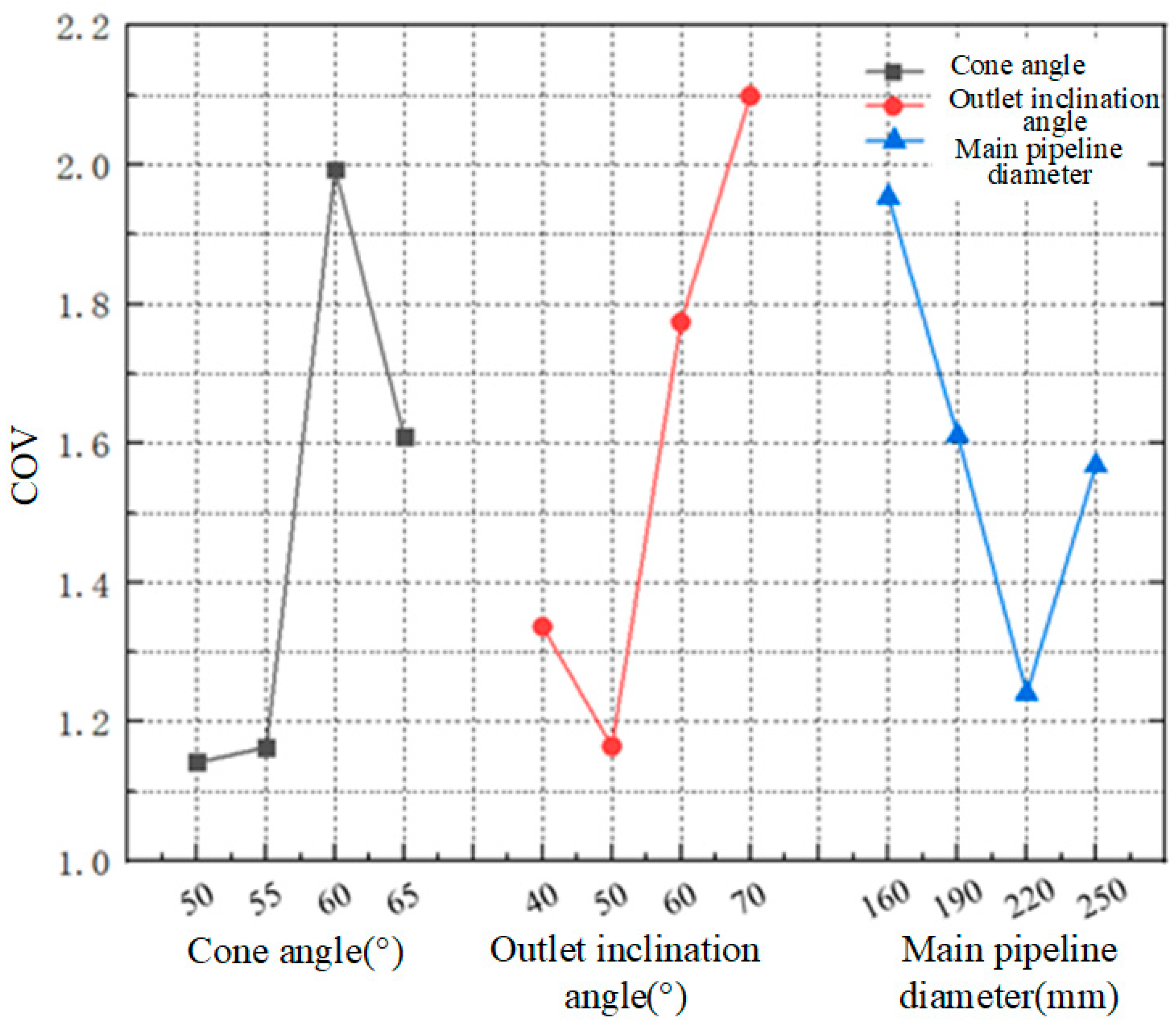
3.2. Orthogonal Experimental Design

In this project, three experimental factors need to be considered simultaneously. If a comprehensive experiment is conducted, the scale of the experiment will be large, and it will be difficult to implement due to time costs. Therefore, the orthogonal experiment method is used for analysis. The orthogonal experiment is an efficient experimental design method that arranges multiple factor experiments and seeks the optimal level combination. It selects some representative level combinations from all level combinations of multi-factor experiments for experimentation, analyzes the results of these experiments to understand the overall situation of the experiment, and finds the optimal level combination. This project adopts a three-factor, four-level experiment and uses orthogonal table L16 (43) to develop a simulation plan.

Table 3. Orthogonal design table.

Number	Mixer Cone Angle (°)/A	Air Inlet Angle (°)/B	Main Pipeline Diameter (mm)/C	Uniformity Index COV Coefficient
1	50	40	160	0.2745
2	50	50	190	0.18148
3	50	60	220	0.291
4	50	70	250	0.3946
5	55	40	190	0.3352
6	55	50	160	0.4409
7	55	60	250	0.394
8	55	70	220	0.4601
9	60	40	220	0.3614
10	60	50	250	0.4141
11	60	60	160	0.606
12	60	70	190	0.6116
13	65	40	250	0.36524
14	65	50	220	0.1282
15	65	60	190	0.4828
16	65	70	160	0.6325

shows the orthogonal design.

To distinguish the data fluctuations caused by changes in experimental conditions from those caused by experimental errors in the experiment, and to provide accurate quantitative estimates of the impact of each factor on the experimental results, an analysis of variance was conducted on the orthogonal experimental results as follows:

Let the experimental result be $CO{V}_i$(i = 1,2,... 16):

$$T={\displaystyle \sum _{i=1}^{16}CO{V}_i}$$

(9)

The sum of squared deviations caused by various factors is as follows:

$$s{s}_{\delta }={\displaystyle \frac{1}{r}}{\displaystyle \sum _{i=1}^4{K}_{ij}{ }^2}-{\displaystyle \frac{T^2}{n}},(j=1,2,3)$$

(10)

where the total number of experiments is n = 16, the level of each factor is m = 4, and each level is repeated r = 4 times; $K_{ij}$ is the sum of the i-th level data in column j; factor number $\delta$ = A, B, C.

The degrees of freedom corresponding to the sum of squared deviations of any factor:

$$df=r-1=3$$

(11)

The variance:

$$M{S}_{\delta }={\displaystyle \frac{s{s}_{\delta }}{df}}$$

(12)

The orthogonal experimental analysis of variance can be obtained as shown in

Table 4. Analysis of orthogonal experiment results.

Analyze Parameters	A	B	C
$K_{1j}$	1.14158	1.33634	1.9539
$K_{2j}$	1.6302	1.16468	1.61108
$K_{3j}$	1.9931	1.7738	1.2407
$K_{4j}$	1.60874	2.0988	1.56794
$K_{1j}^2$	1.3032	1.7858	3.81773
$K_{2j}^2$	2.65755	1.35648	2.59558
$K_{3j}^2$	3.97245	3.15908	1.53934
$K_{4j}^2$	2.58804	4.405	2.45843
${SS}_{\delta }$	0.09141	0.13769	0.06387
${MS}_{\delta }$	0.03047	0.046	0.02129
Proportion of ${MS}_{\delta }$ (%)	31.168	47.054	21.778

.

As shown in the table above, the primary and secondary order of the influencing factors on the COV value of the uniformity coefficient is the inclination angle of the air outlet, the cone angle, and the diameter of the main pipeline. The proportion of these influencing factors is 0.4705:0.3117:0.2177, respectively. From the above analysis, it can be concluded that the inclination angle of the air outlet should be determined based on the size of the cone angle. Therefore, when designing the mixer, the optimal cone angle should be selected first, followed by the inclination angle of the air outlet that is close to the cone angle, and finally, the appropriate diameter of the main pipeline should be considered.

Figure 14 shows the influence of a single factor on the mixing effect. From the graph, it can be seen that the overall mixing effect is better when the cone angle is 55°, the outlet inclination angle is closest to 55°, and the main pipeline diameter is 190 mm, which is consistent with the analysis results of controlling single-factor variables.

The comparison of the uniformity coefficient COV values obtained from the above orthogonal experiments shows that the mixing uniformity is the best, that is, the combination of the two mixers with the lowest COV coefficient—namely, the cone angle, outlet inclination angle, and main pipeline diameter structure—is 65-50-220 and 50-50-190. Therefore, it can be inferred that the optimal mixer structure combination in practical applications is 50-50-220.

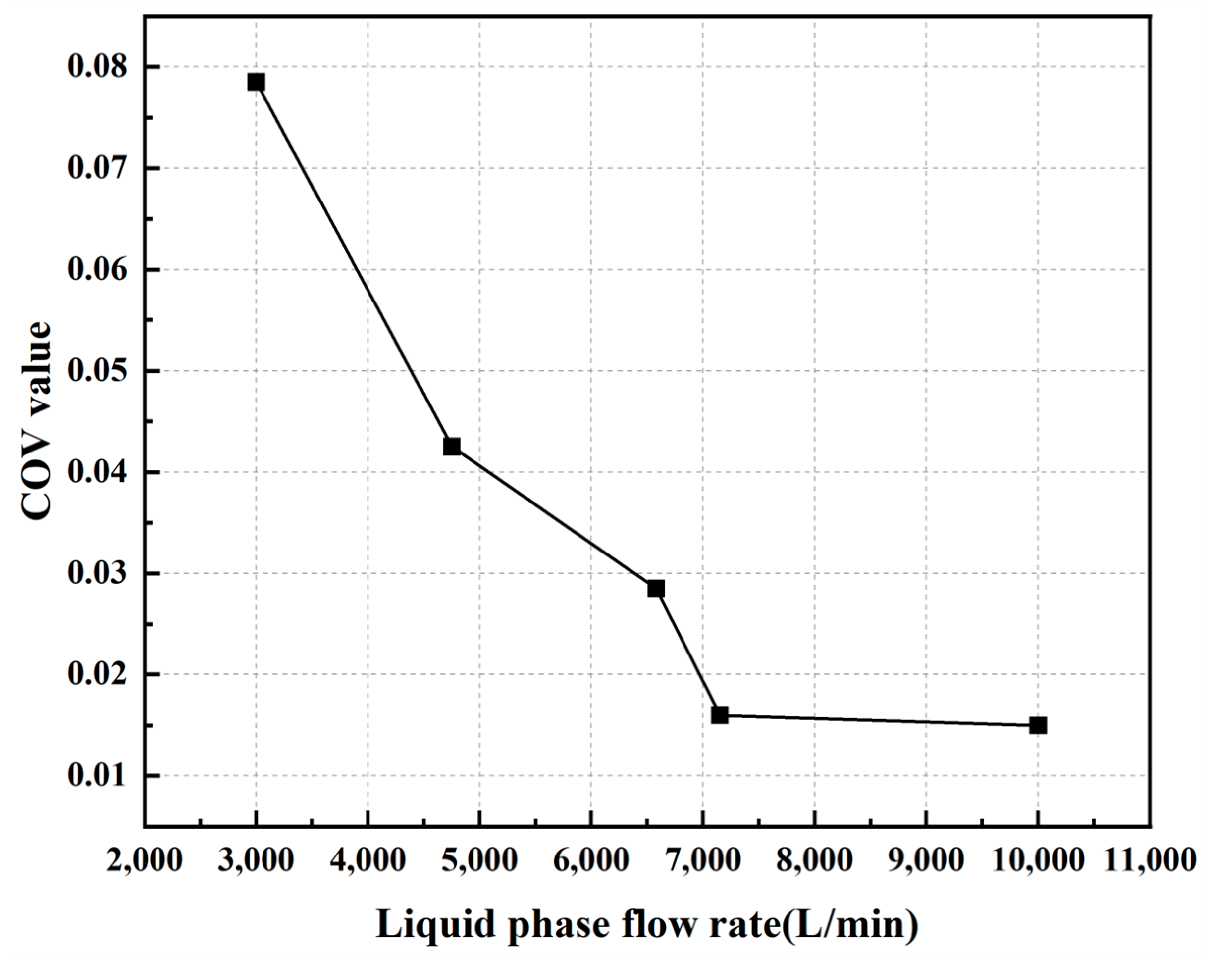
3.3. The Impact of Flow Rate on the Mixing Effect

Since the above research object is aimed at the working condition of a liquid phase flow rate of 10,000 L/min, to explore the change in gas–liquid mixing effect under the condition of small flow rate, and to clarify the influence of flow rate change on the optimal mixing pipe diameter and the shortest straight pipe length required for uniform mixing, a 10 m long gas–liquid mixer with a cone angle of 60°, an outlet inclination angle of 60°, and a main pipe diameter of 250 mm is selected as the simulation model. Based on this model, we, respectively, control the foam liquid flow rate to 10,000 L/min, 7200 L/min, 6600 L/min, 4800 L/min, and 3000 L/min for numerical simulation, and monitor and calculate the COV value of the uniformity coefficient of liquid volume fraction of each section. The obtained simulation results are fitted with curves to obtain the variation law of the best pipe diameter and the shortest mixing distance with the flow rate.

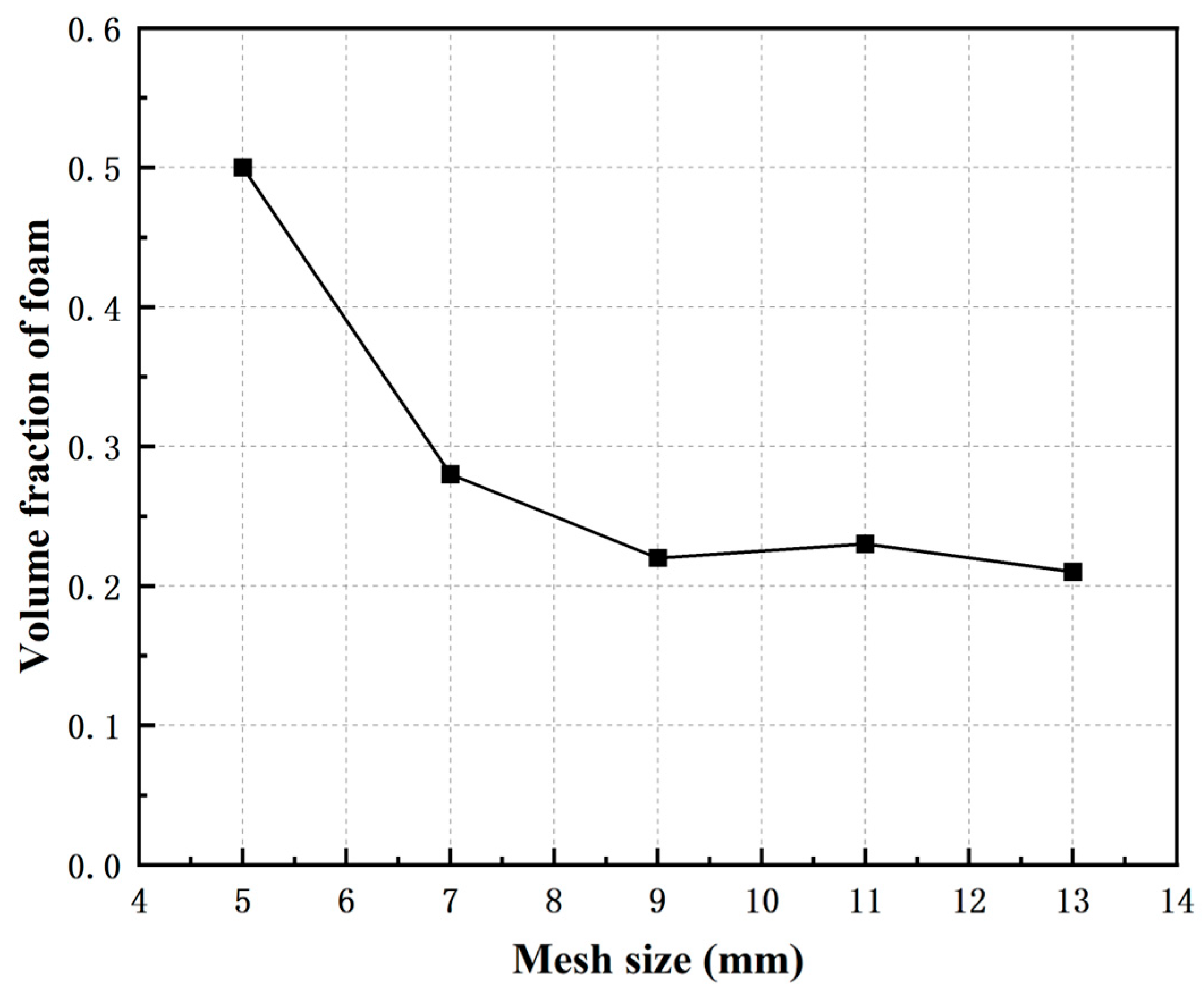
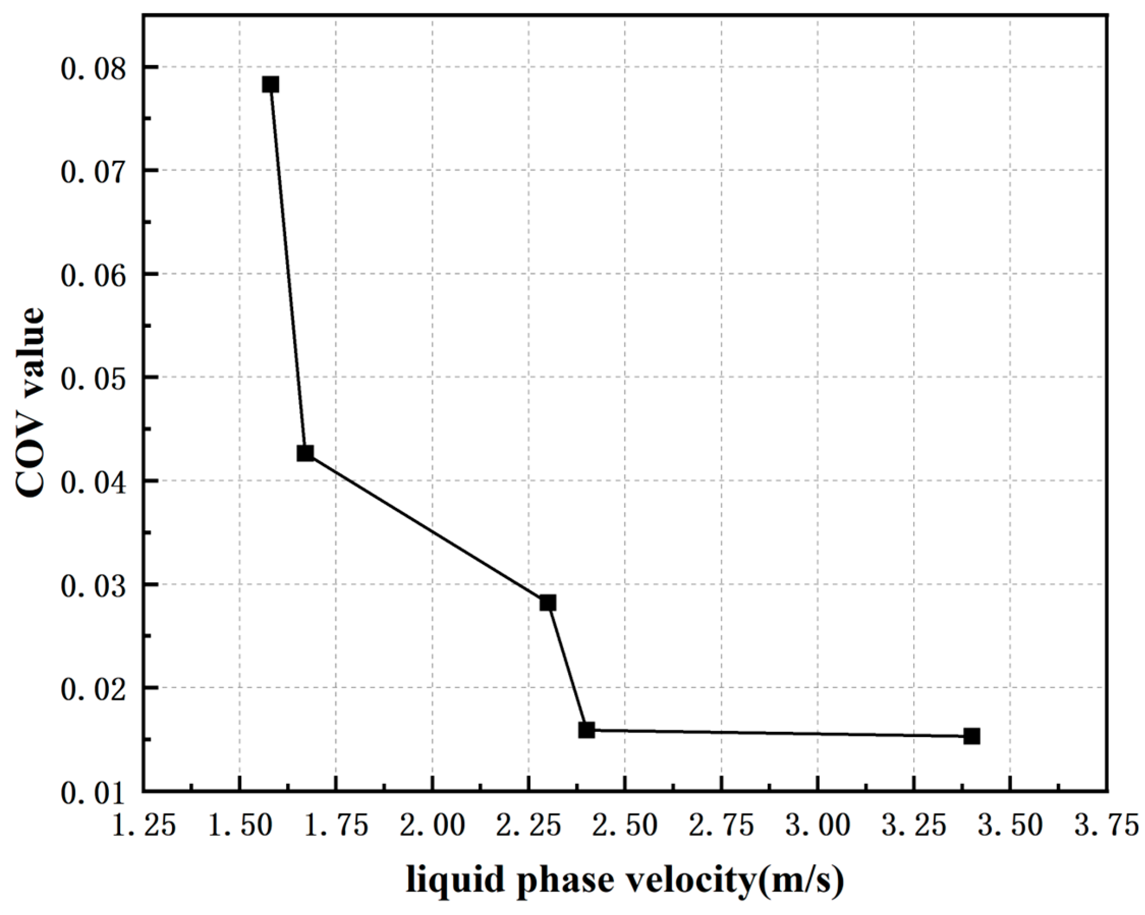
3.3.1. Impact of Flow Rate on Optimal Pipe Diameter

Figure 15 shows the distribution of the COV coefficient for liquid phase volume fraction at outlet cross-sections under different flow rates. It can be seen from the figure that under the same and larger pipe diameter, the higher the fluid flow rate and the higher the foam liquid speed, the better the mixing uniformity. However, this phenomenon becomes less obvious after the liquid flow rate reaches 7200 L/min. Therefore, it can be concluded that using a larger flow rate can achieve better mixing effects under the same pipe diameter, but the promoting effect on the mixing effect becomes less significant when the flow rate is too high.

Due to the direct correlation between pipe diameter and liquid phase velocity, the appropriate velocity can be selected when determining the flow rate, and the corresponding optimal pipe diameter can be selected through calculation.

Convert Figure 15 into a COV value velocity line, as shown in Figure 16.

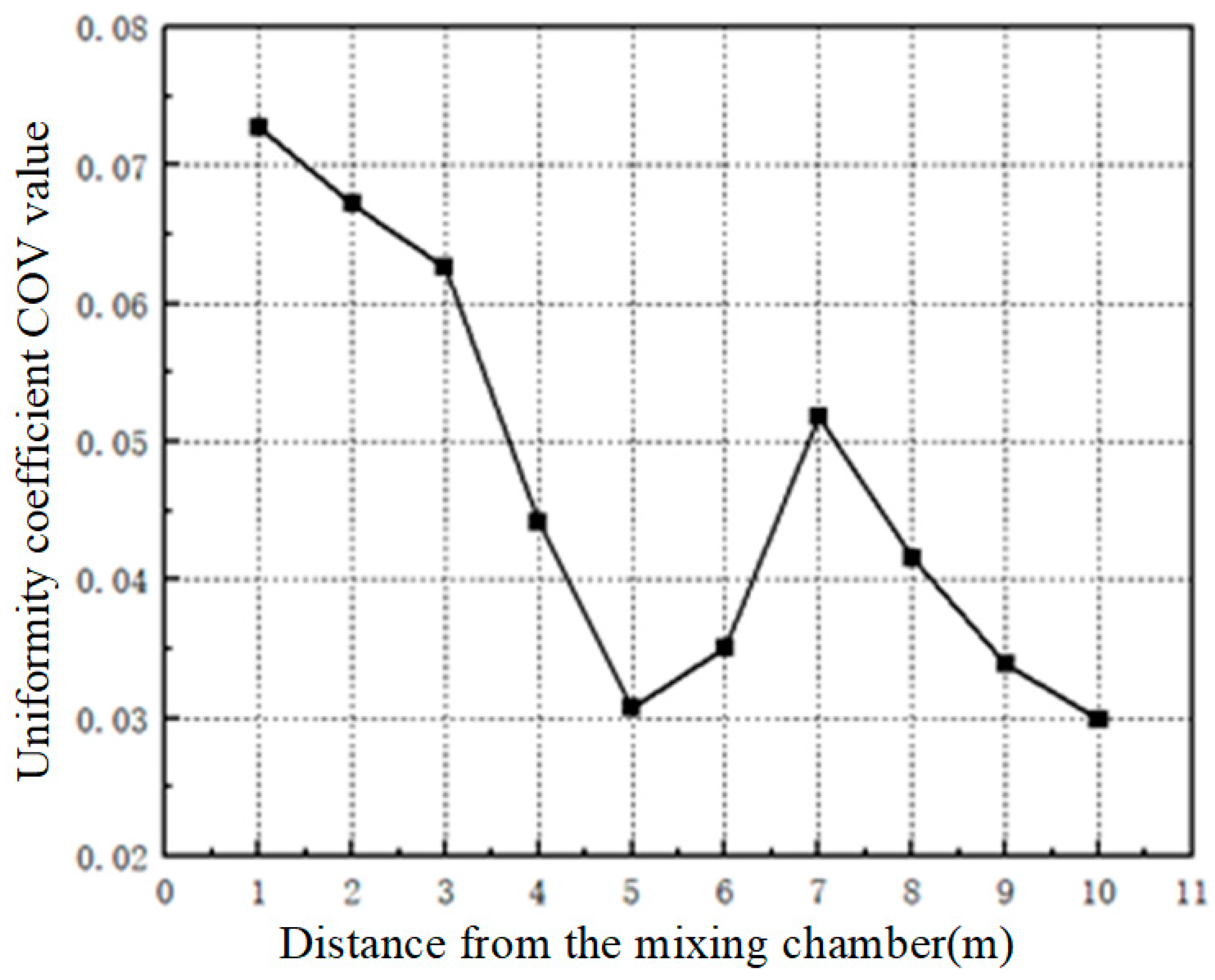
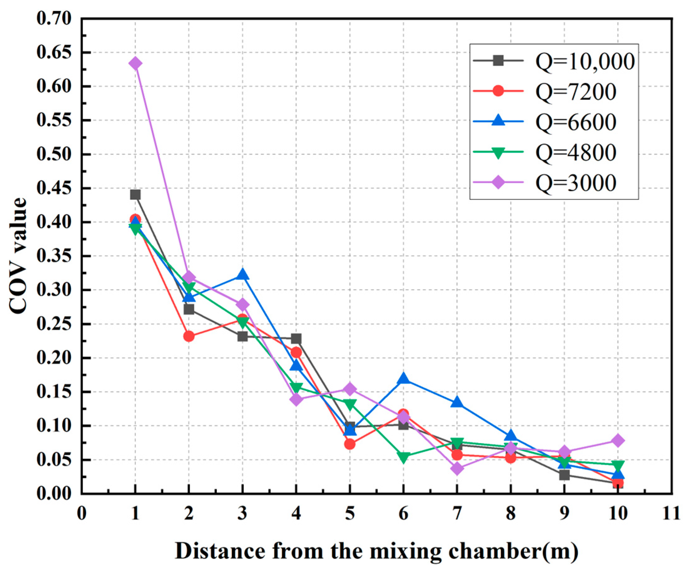
3.3.2. Impact of Flow Rate on the Shortest Mixing Distance

We set monitoring points every 1 m on the backend pipeline of the gas–liquid mixing device model, measured the COV coefficient of the liquid phase to observe the degree of mixing uniformity, and obtained the simulation results shown in Figure 17.

From Figure 17, it can be seen that as the mixing distance increases, the COV value decreases, indicating that the mixing is becoming more uniform. The effect of flow rate on mixing uniformity is indeed not significant.

4. Conclusions

Through simulation research on the actual vehicle model of the JP21/G2 fire truck, the results show that the presence of bent pipes hinders the gas–liquid mixing process and reduces the mixing effect. It is recommended to arrange pipelines reasonably and avoid the appearance of bent pipes as much as possible. Through orthogonal experiments, the optimal parameter combination with an accurate value of 50°-50°-220 mm was obtained.

Through variable flow simulation experiments, it can be concluded that under the same pipe diameter, using a larger flow rate can achieve better mixing effects, but the promoting effect on the mixing effect becomes less significant when the flow rate is too high. The impact of flow on the shortest mixing distance is that the smaller the flow, the smaller the required shortest mixing pipe length, but this effect is less significant.

This paper mainly studies the influence of structural parameters of the optimized model of the gas–liquid mixing device of the JP21/G2 fire truck on the gas–liquid mixing effect. The research results have important economic and social benefits, but the manuscript does not consider the influence of simulation boundary conditions, gas–liquid ratio, foam liquid viscosity on energy loss, and mixing effect, which is a problem to be solved.

References

1. Georgiadis-Filikas, K.; Bakas, I.; Kontoleon, K. Statistical Analysis and Review of Fire Incidents Data of Greece, with Special Focus on Residential Cases 2000–2019. Fire Technol. 2022, 58, 3191–3233. [Google Scholar] [CrossRef]
2. Luo, Y.; Li, Q.; Jiang, L.; Zhou, Y. Analysis of Chinese fire statistics during the period 1997–2017. Fire Safety J. 2021, 125, 103400. [Google Scholar] [CrossRef]
3. Jin, G.; Wang, Q.; Zhu, C.; Feng, Y.; Huang, J.; Hu, X. Urban Fire Situation Forecasting: Deep sequence learning with spatio-temporal dynamics. Appl. Soft Comput. 2020, 97, 106730. [Google Scholar] [CrossRef]
4. Luo, R.; Hui, D.; Miao, N.; Liang, C.; Wells, N. Global relationship of fire occurrence and fire intensity: A test of intermediate fire occurrence-intensity hypothesis. J. Geophys. Res. Biogeosci. 2017, 122, 1123–1136. [Google Scholar] [CrossRef]
5. Guo, T.; Fu, Z. The fire situation and progress in fire safety science and technology in China. Fire Safety J. 2007, 42, 171–182. [Google Scholar] [CrossRef]
6. Cheung, W.K.; Zeng, Y.; Lin, S.; Huang, X. Modelling carbon monoxide transport and hazard from smouldering for building fire safety design analysis. Fire Safety J. 2023, 140, 103895. [Google Scholar] [CrossRef]
7. Bai, M.; Liu, Q. Evaluating Urban Fire Risk Based on Entropy-Cloud Model Method Considering Urban Safety Resilience. Fire 2023, 6, 62. [Google Scholar] [CrossRef]
8. Hulse, L.M.; Galea, E.R.; Thompson, O.F.; Wales, D. Perception and recollection of fire hazards in dwelling fires. Safety Sci. 2020, 122, 104518. [Google Scholar] [CrossRef]
9. Chaos, M. Determination of Separation Distances Inside Large Buildings. Fire Technol. 2017, 53, 249–281. [Google Scholar] [CrossRef]
10. Cheng, L.; Li, S.; Ma, L.; Li, M.; Ma, X. Fire spread simulation using GIS: Aiming at urban natural gas pipeline. Safety Sci. 2015, 75, 23–35. [Google Scholar] [CrossRef]
11. Wang, B.; Li, W.; Lai, G.; Chang, N.; Chen, F.; Bai, Y.; Liu, X. Forest Fire Spread Hazard and Landscape Pattern Characteristics in the Mountainous District, Beijing. Forests 2023, 14, 2139. [Google Scholar] [CrossRef]
12. Jiao, Q.; Fan, M.; Tao, J.; Wang, W.; Liu, D.; Wang, P. Forest Fire Patterns and Lightning-Caused Forest Fire Detection in Heilongjiang Province of China Using Satellite Data. Fire 2023, 6, 166. [Google Scholar] [CrossRef]
13. Ma, W.; Feng, Z.; Cheng, Z.; Chen, S.; Wang, F. Identifying Forest Fire Driving Factors and Related Impacts in China Using Random Forest Algorithm. Forests 2020, 11, 507. [Google Scholar] [CrossRef]
14. Li, X.; Liu, L.; Qi, S. Forest fire hazard during 2000–2016 in Zhejiang province of the typical subtropical region, China. Nat. Hazards 2018, 94, 975–977. [Google Scholar] [CrossRef]
15. Grishin, A.M.; Filkov, A.I. A deterministic-probabilistic system for predicting forest fire hazard. Fire Safety J. 2011, 46, 56–62. [Google Scholar] [CrossRef]
16. Yin, H.; Kong, F.; Li, X. RS and GIS-based forest fire risk zone mapping in da hinggan mountains. Chinese Geogr. Sci. 2004, 14, 251–257. [Google Scholar] [CrossRef]
17. Chen, F.; Xu, T.; Hou, G.; Huang, J.; Zhu, G.; Deng, T.; Jiang, Z.; Wang, Z. Efficiency and mechanism of fire suppression through pneumatic sandblasting firefighting. Case Stud. Therm. Eng. 2023, 49, 103361. [Google Scholar] [CrossRef]
18. Wang, W.; He, S.; He, T.; You, T.; Parker, T.; Wang, Q. Suppression behavior of water mist containing compound additives on lithium-ion batteries fire. Process Saf. Environ. 2022, 161, 476–487. [Google Scholar] [CrossRef]
19. Sheng, Y.; Xue, M.; Ma, L.; Zhao, Y.; Wang, Q.; Liu, X. Environmentally Friendly Firefighting Foams Used to Fight Flammable Liquid Fire. Fire Technol. 2021, 57, 2079–2096. [Google Scholar] [CrossRef]
20. Aydin, B.; Selvi, E.; Tao, J.; Starek, M. Use of Fire-Extinguishing Balls for a Conceptual System of Drone-Assisted Wildfire Fighting. Drones 2019, 3, 17. [Google Scholar] [CrossRef]
21. Deng, B.; Lu, L.; Qian, X.; Kang, Q.; Fu, L. Research on the influence of driving gas types in compound jet on extinguishing the pool fire. J. Hazard. Mater. 2019, 363, 152–160. [Google Scholar] [CrossRef] [PubMed]
22. Yuan, F.; Cui, Z.; Lin, J. Experimental and Numerical Study on Flow Resistance and Bubble Transport in a Helical Static Mixer. Energies 2020, 13, 1228. [Google Scholar] [CrossRef]
23. Jia, X.; Che, B.; Jing, G.; Zhang, C. Air-Bubble Induced Mixing: A Fluidic Mixer Chip. Micromachines 2020, 11, 195. [Google Scholar] [CrossRef] [PubMed]
24. Hashemi, N.; Ein-Mozaffari, F.; Upreti, S.R.; Hwang, D.K. Experimental investigation of the bubble behavior in an aerated coaxial mixing vessel through electrical resistance tomography (ERT). Chem. Eng. J. 2016, 289, 402–412. [Google Scholar] [CrossRef]
25. Dietrich, N.; Poncin, S.; Midoux, N.; Li, H.Z. Bubble formation dynamics in various flow-focusing microdevices. Langmuir 2008, 24, 13904–13911. [Google Scholar] [CrossRef] [PubMed]
26. Zhou, W.; Wang, H.; Wang, L.; Li, L.; Cai, C.; Zhu, J. The Law of Gas–Liquid Shear Mixing under the Synergistic Effect of Jet Stirring. Processes 2023, 11, 2531. [Google Scholar] [CrossRef]
27. Liu, Y.; Guo, J.; Li, W.; Li, W.; Zhang, J. Investigation of gas-liquid mass transfer and power consumption characteristics in jet-flow high shear mixers. Chem. Eng. J. 2021, 411, 128580. [Google Scholar] [CrossRef]
28. Amiri, T.Y.; Moghaddas, J.S.; Moghaddas, Y. A jet mixing study in two phase gas–liquid systems. Chem. Eng. Res. Des. 2011, 89, 352–366. [Google Scholar] [CrossRef]
29. Hou, J.; Qian, G.; Zhou, X. Gas–liquid mixing in a multi-scale micromixer with arborescence structure. Chem. Eng. J. 2011, 167, 475–482. [Google Scholar] [CrossRef]
30. Khopkar, A.R.; Kasat, G.R.; Pandit, A.B.; Ranade, V.V. CFD simulation of mixing in tall gas–liquid stirred vessel: Role of local flow patterns. Chem. Eng. Sci. 2006, 61, 2921–2929. [Google Scholar] [CrossRef]
31. Meroney, R.N.; Colorado, P.E. CFD simulation of mechanical draft tube mixing in anaerobic digester tanks. Water Res. 2009, 43, 1040–1050. [Google Scholar] [CrossRef]
32. Liu, Y.; Mitchell, T.; Upchurch, E.R.; Ozbayoglu, E.M.; Baldino, S. Investigation of Taylor bubble dynamics in annular conduits with counter-current flow. Int. J. Multiphas Flow 2024, 170, 104626. [Google Scholar] [CrossRef]
33. Liu, Y.; Ozbayoglu, E.M.; Upchurch, E.R.; Baldino, S. Computational fluid dynamics simulations of Taylor bubbles rising in vertical and inclined concentric annuli. Int. J. Multiph. Flow 2023, 159, 104333. [Google Scholar] [CrossRef]
34. Xu, L.; Yu, B.; Wang, C.; Jiang, H.; Liu, Y.; Chen, R. Particle-resolved CFD simulations of local bubble behaviors in a mini-packed bed with gas–liquid concurrent flow. Chem. Eng. Sci. 2022, 254, 117631. [Google Scholar] [CrossRef]
35. Ning, J.; Jin, Z.; Xu, X. A partition-coupled Eulerian–Lagrangian method for large-deformation simulation of compressible fluid. Phys. Fluids 2022, 34, 116102. [Google Scholar] [CrossRef]
36. Gómez-Pastora, J.; González-Fernández, C.; Fallanza, M.; Bringas, E.; Ortiz, I. Flow patterns and mass transfer performance of miscible liquid-liquid flows in various microchannels: Numerical and experimental studies. Chem. Eng. J. 2018, 344, 487–497. [Google Scholar] [CrossRef]
37. Shao, N.; Gavriilidis, A.; Angeli, P. Flow regimes for adiabatic gas–liquid flow in microchannels. Chem. Eng. Sci. 2009, 64, 2749–2761. [Google Scholar] [CrossRef]
38. Hu, J.; Li, W.; Chi, X.; Wang, N. Study on the Effect of Structural Parameters of Volume Control Tank on Gas–Liquid Mass Transfer. Energies 2023, 16, 4991. [Google Scholar] [CrossRef]
39. Van Reeuwijk, M.; Sookhak Lari, K. Asymptotic solutions for turbulent mass transfer at high Schmidt number. Proc. R. Soc. A Math. Phys. Eng. Sci. 2012, 468, 1676–1695. [Google Scholar] [CrossRef]
40. Vijiapurapu, S.; Cui, J. Performance of turbulence models for flows through rough pipes. Appl. Math. Model. 2010, 34, 1458–1466. [Google Scholar] [CrossRef]
41. Mohammed, H.I.; Giddings, D.; Walker, G.S. CFD simulation of a concentrated salt nanofluid flow boiling in a rectangular tube. Int. J. Heat. Mass. Tran. 2018, 125, 218–228. [Google Scholar] [CrossRef]
42. Fan, Z.; Liu, D.; Pan, S.; Ma, J.; Chen, X. Spreading dynamics of the viscous droplet impacting on a spherical particle. Phys. Fluids 2023, 35, 023311. [Google Scholar] [CrossRef]
43. Wang, W.; Lin, F.; Wei, X.; Zou, J. Antibubble formation by a single drop impact on a free surface. Phys. Fluids 2021, 33, 042107. [Google Scholar] [CrossRef]
44. Zhou, Y.; Chang, H.; Qi, T. Gas–liquid two-phase flow in serpentine microchannel with different wall wettability. Chinese J. Chem. Eng. 2017, 25, 874–881. [Google Scholar] [CrossRef]
45. Sun, B.; Lu, Y.; Liu, Q.; Fang, H.; Zhang, C.; Zhang, J. Experimental and Numerical Analyses on Mixing Uniformity of Water and Saline in Pipe Flow. Water 2020, 12, 2281. [Google Scholar] [CrossRef]
Figure 1. Division of outlet cross-section.
Processes 12 01707 g001
Figure 2. Fluid domain model of gas–liquid mixing device.
Processes 12 01707 g002
Figure 3. Structural diagram of the gas–liquid mixing device.
Processes 12 01707 g003
Figure 4. Study on mesh independence.
Processes 12 01707 g004
Figure 5. Comparison of normalized pressure drop at the front and rear ends of the mixing chamber.
Processes 12 01707 g005
Figure 6. Three views of the JP21/G2 numerical simulation model: (a) front view; (b) left view; (c) top view.
Processes 12 01707 g006
Figure 7. Contour of liquid phase volume fraction at outlet end face under different mixing durations.
Processes 12 01707 g007
Figure 8. Variation in liquid phase volume fraction with mixing distance at 2.4 s.
Processes 12 01707 g008
Figure 9. Variation in COV value with mixing distance at 2.4 s.
Processes 12 01707 g009
Figure 10. Liquid phase volume fraction contours with different cross-sections.
Processes 12 01707 g010
Figure 11. Static pressure contours of different cross-sections.
Processes 12 01707 g011
Figure 12. Velocity streamlines at the front end of a bent pipe.
Processes 12 01707 g012
Figure 13. Velocity streamlines at the rear end of a bent pipe.
Processes 12 01707 g013
Figure 14. Single-factor influence diagram of orthogonal experiment.
Processes 12 01707 g014
Figure 15. Variation in COV value with liquid phase flow rate.
Processes 12 01707 g015
Figure 16. Variation in COV value with liquid phase velocity.
Processes 12 01707 g016
Figure 17. Variation in COV value with mixing distance under different flow rates.
Processes 12 01707 g017