Study on Short-Term Electricity Load Forecasting Based on the Modified Simplex Approach Sparrow Search Algorithm Mixed with a Bidirectional Long- and Short-Term Memory Network

Abstract

In order to balance power supply and demand, which is crucial for the safe and effective functioning of power systems, short-term power load forecasting is a crucial component of power system planning and operation. This paper aims to address the issue of low prediction accuracy resulting from power load volatility and nonlinearity. It suggests optimizing the number of hidden layer nodes, number of iterations, and learning rate of bi-directional long- and short-term memory networks using the improved sparrow search algorithm, and predicting the actual load data using the load prediction model. Using actual power load data from Wuxi, Jiangsu Province, China, as a dataset, the model makes predictions. The results indicate that the model is effective because the enhanced sparrow algorithm optimizes the bi-directional long- and short-term memory network model for predicting the power load data with a relative error of only 2%, which is higher than the prediction accuracy of the other models proposed in the paper.

1. Introduction

Electricity is a special kind of secondary energy that is produced, transmitted, distributed and consumed simultaneously. This means that power generation on the supply side and power consumption on the user side are in a dynamic equilibrium relationship. When power generation and consumption are not balanced, it can cause safety accidents and lead to large economic losses for the power system and users. Given the characteristics of electric energy and the randomness of load changes, the accurate forecasting of power loads and predicting trends in advance can help the power sector make timely and scientific decisions, guaranteeing the electrical grid’s continuous, secure, and reliable functioning.

Power load and past climatic data are the foundations of power load forecasting. This explores the change rule of power load history and predicts future load based on this analysis. Based on the time horizon, power load forecasting is separated into four categories: ultra-short-term, short-term, medium-term, and long-term. Long-term power load forecasting covers the next three to five years and provides a basis for grid planning departments in their vision planning [1,2]. Medium-term power load forecasting covers the next one month to one year and provides a reference for equipment maintenance plans. Short-term power load forecasting covers the next few hours to a few days and can be used for grid arrangement and scheduling plans [3,4]. Ultra-short-term power load forecasting covers a time range of one hour in the future and can be used for preventive emergency control and handling of emergencies.

The goal of current research on short-term power load prediction has been to increase prediction accuracy. Numerous conventional techniques, including regression analysis, time series, and comparable day approaches, have been employed in earlier research. But these methods usually have some limitations, such as low accuracy, weak ability to integrate influencing factors and low sensitivity to input data. With the fast growth of computer science and artificial intelligence, machine learning approaches have been brought into the field of short-term power demand forecasting. These methods comprise random forests (RF), support vector machines (SVM), artificial neural networks (ANN), and long- and short-term memory networks (LSTM). These approaches make up for the drawbacks of standard load forecasting methods, increase the accuracy of short-term power load prediction, and present fresh concepts for short-term power load forecasting.

A long- and short-term memory network is a form of recurrent neural network (RNN) architecture utilized in the field of machine learning, which is ideal for the classification, manufacturing, and prediction of time series data. Research academics at home and abroad have applied LSTM to the field of load forecasting in recent years by analyzing the influence of important factors such as meteorology and regional economy and constructing and improving forecasting models [5,6,7]. Reference [8] proposed a short-term power load forecasting method based on a convolutional neural network (CNN) and a long- and short-term memory network (LSTM), which employs CNN to extract the feature vectors of the input data, and the feature vectors are utilized as inputs to the LSTM forecasting model. Better forecasting results are achieved by analyzing the example of the power load in Bangladesh, but both CNN and LSTM require a large amount of computation, which requires strong hardware support, and the setting of too many parameters is also a major problem. In reference [9], to increase the accuracy of short-term power load forecast, the article adopts the variational modal decomposition (VMD) method to decompose the original power load data signals, and then the deconstructed sub-signals and the original signals are formed into a new dataset fed into the neural network for training so that the artificial neural network can learn more information, and its ability to predict is more outstanding, but the sub-signals after the decomposition of VMD usually lack intuitive interpretation, which can make the prediction results difficult to understand. Reference [10] proposed a discrete particle swarm (DPSO)-optimized short-term power load prediction model for a long- and short-term memory network (LSTM), which employs the DPSO technique to improve the parameters of the LSTM model, and in the case study, real data from four provinces in central China are used to test the efficiency of the suggested model, but DPSO may encounter the dimension disaster problem.

LSTM can learn historical knowledge and has a memory function for historical information. However, it only has the ability to acquire forward knowledge and cannot acquire backward information well. To make each moment contain contextual information, some scholars have proposed a bi-directional long- and short-term memory network (BiLSTM) by combining the bi-directional recurrent neural network (BIRNN) model with the LSTM unit. The BiLSTM is an upgrade of the LSTM, which not only absorbs forward information but also employs backward information efficiently [11]. Reference [12] proposed an improved prediction model for BiLSTM: the authors used improved particle swarm optimization (IPSO) to improve the settings of BiLSTM, and the experimental findings demonstrate that the IPSO-BiLSTM model has superior prediction outcomes to the LSTM model and BiLSTM model. Reference [13] developed a short-term power load forecasting approach based on an attention system and simultaneous long- and short-term memory network. It leverages the attention mechanism to emphasize the input elements that play a crucial role in load forecasting and then combines with the BiLSTM model for forecasting, which achieved better forecasting results in the example simulation, but its complexity is too high.

In this study, we propose the creation of a novel short-term power load forecasting approach utilizing the modified simplex approach sparrow search algorithm (SMSSA) mixed with a bidirectional long- and short-term memory network (BiLSTM). The approach leverages the SMSSA algorithm to maximize the number of hidden layer nodes, the number of iterations, and the learning rate of BiLSTM, and to decrease the uncertainty of manual trial settings. Finally, simulation analysis is carried out utilizing data from the Wuxi region in Jiangsu Province, China, and the analysis findings suggest that the approach described in this research has a strong prediction performance.

2. Long- and Short-Term Memory Networks

Long- and short-term memory (LSTM) is an upgraded recurring neural network proposed by Hochreiter and Schmid Huber in 1997 [14]. LSTM avoids the problem of gradient vanishing of ordinary RNNs when confronting long-term dependencies, and it is an efficient RNN design. Figure 1 demonstrates the basic framework of LSTM.

LSTM introduces the concepts of gates and memory cells in each hidden layer. The forgetting gate deletes old input data and resets the memory unit; the input gate adds fresh valid information to the memory unit; and the output gate activates the valid information for filtering and output to the succeeding network. This approach of managing the memory units by three gating units overcomes the problem that RNNs cannot acquire long-distance temporal relationships and successfully mitigates the gradient vanishing problem [15,16,17]. This makes LSTM an appropriate neural network topology for tackling the long-term dependence problem. The state update equations for the basic units of LSTM are shown in Equations (1)–(6):

$$f_t=\sigma \left(W_f\right[h_{t-1}, x_t\left]\right)+b_f$$

(1)

$$i_t=\sigma (W_i\cdot [h_{t-1}, x_t\left]\right)+b_i$$

(2)

$${\widehat{C}}_t=\mathit{tan}h(W_c\cdot [h_{t-1}, x_t])+b_c$$

(3)

$$C_t=f_t\circ C_{t-1}+i_t\circ {\widehat{C}}_t$$

(4)

$$o_t=\sigma (W_o\cdot [h_{t-1}, x_t\left]\right)+b_o$$

(5)

$$h_t=o_t\circ \mathit{tan}h{C}_t$$

(6)

where $x_t$ is the input at time t; $f_t$, $i_t$ and $o_t$ denote the forgetting gate, the input gate, and the output gate, respectively; $a_t$ is the input node state at time t; $C_{t-1}$ and $C_t$ are the cell states at time t − 1 and time t, respectively; $h_{t-1}$ and $h_t$ are the outputs at time t − 1 and time t, respectively; $\sigma$ is the sigmoid activation function; tanh is the hyperbolic tangent function;$W_f$, $W_i$, $W_c$ and $b_f$, $b_i$, $b_c$, $b_o$ are the corresponding weight matrices and bias vectors; and $\circ$ denotes the Hadamard product.

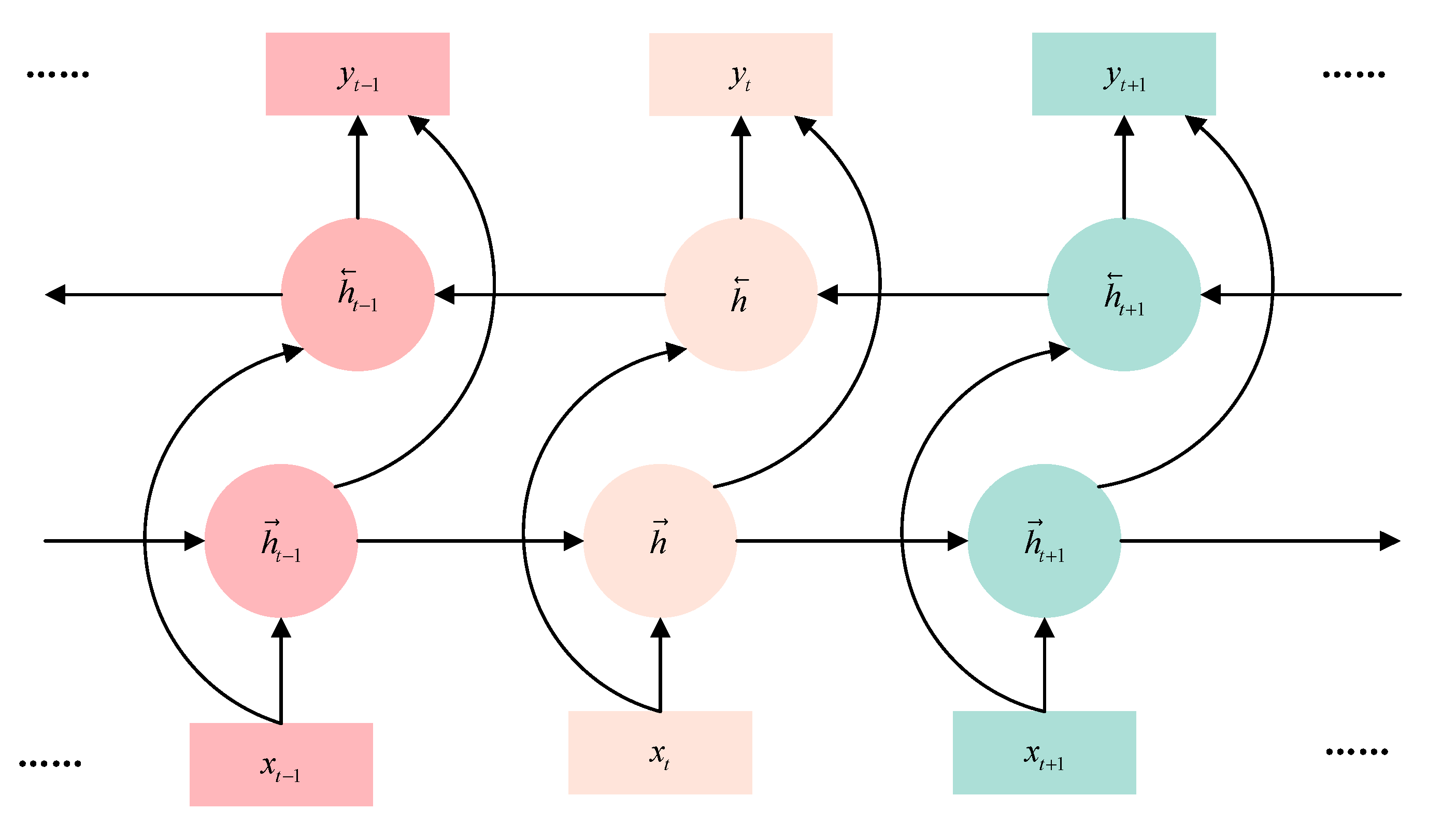
3. Bidirectional Long- and Short-Term Memory Networks

LSTM can learn historical knowledge and has a memory function for historical information. However, it only has the ability to acquire the forward knowledge and cannot acquire the backward information well. To learn contextual information at each moment, several academics have merged the bidirectional recurrent neural network (BiRNN) model with LSTM units for gathering contextual information and have suggested the bidirectional long- and short-term memory network model.

The bidirectional long- and short-term memory (BiLSTM) network model is an improvement of the LSTM network, which not only learns the forward information but also utilizes the backward information effectively [18]. The framework of BiLSTM is given in Figure 2.

As shown in Figure 2, the BiLSTM neural network has two directions of hidden layers, a pre-hidden layer forward training time series and a post-hidden layer backward training time series, and both the pre-transmission and post-transmission layers are connected to the output layer. x is the model input, h is the hidden layer state, and y is the output. The BiLSTM operation is as follows:

$${\stackrel{r}{h}}_t=f(\stackrel{r}{w}·x_t+\stackrel{r}{v}·{\stackrel{r}{h}}_{t-1}+\stackrel{r}{b})$$

(7)

$${\stackrel{s}{h}}_t=f(\stackrel{s}{w}·x_t+\stackrel{s}{v}·{\stackrel{s}{h}}_{t-1}+\stackrel{s}{b})$$

(8)

$$y_t=g(U[\stackrel{r}{h_{\mathrm{t}}},\stackrel{s}{h_{\mathrm{t}}}]+c)$$

(9)

where ${\stackrel{r}{h}}_t$ and ${\stackrel{ r}{h}}_{t-1}$ denote the forward LSTM hidden layer states at moments t and t − 1, respectively; ${\stackrel{s}{h}}_t$ and ${\stackrel{s}{h}}_{t-1}$ denote the reverse LSTM hidden layer states at moments t and t − 1, respectively; $\stackrel{r}{w}$, $\stackrel{r}{v}$, $\stackrel{s}{w}$ and $\stackrel{s}{v}$ are the corresponding weights; $\stackrel{r}{ b}$, $\stackrel{s}{ b}$ are the corresponding biases; $x_t$ is the input at moment t; and $y_t$ is the output at moment t.

4. Improving Sparrow Search Algorithm to Optimize Bidirectional Long- and Short-Term Memory Networks

The power load sequence is fundamentally time-series data containing interconnected earlier and post-input power load data, which is useful for creating a suitable short-term power load forecasting model employing bidirectional long- and short-term memory networks. When employing the BiLSTM model for short-term power load prediction, the learning rate and the number of training times have a very big influence on the model prediction performance. The learning rate influences whether the model can successfully converge to the ideal value, and choosing too big a learning rate will make the model oscillate and not converge at the optimal value, while choosing too small a learning rate will make the model training very slow and reduce the efficiency of the model operation [19]. The selection of the number of training times has a major impact on the model fitting: setting the number of training times too high eventually produces model overfitting, whereas if the number of training times is too little, the curve-fitting effect may not be good. Furthermore, the performance of the model is also influenced by the neural network structure. The BiLSTM model’s structure can be optimized by choosing the right number of hidden layer layers and nodes. Through this process, the model can reach its optimal performance [20]. Therefore, in this study, an enhanced sparrow search algorithm (SMSSA) is utilized to automate the parameter selection of the BiLSTM model to increase the prediction accuracy and model generalization of the BiLSTM model.

4.1. Principles of Sparrow Search Algorithm

The sparrow search method (SSA) is a unique optimization method introduced by Jiankai Xue in 2020, which gives a new way to handle complicated global optimization issues [21]. Sparrows are flocking birds and have strong memory compared to other birds. There is a definite division of work within the sparrow’s population: one portion is termed the discoverer, and the other part is called the follower. The finders are responsible for locating food and providing the populace with foraging places and guidance, while the followers receive food through the finders. The behavior of sparrows can be described as follows:

Step 1: Finders often have large amounts of energy reserves and supply forage locations and search routes for anyone searchers.

Step 2: When a sparrow discovers a predator, it emits a warning signal. When the warning signal is bigger than a safety threshold, the finder moves all followers into a safe region.

Step 3: Every sparrow has the potential to be a finder, provided a good food source can be provided. The ratio of discoverers to followers remains constant throughout the population.

Step 4: Sparrows with greater access to food will act as producers. To obtain more food, hungry followers will likely fly elsewhere to forage for more food.

Step 5: Followers follow the best finder in search of food. Additionally, there will be predators that may continually observe the finders and compete for food.

Step 6: Sparrows in the middle of the group move swiftly to a safe region to acquire a better position when they confront danger, whereas those in the middle of the group approach other sparrows randomly.

A sparrow search algorithm may be created using a mathematical model thanks to the behavioral description of sparrows. Assuming that there is a population of N sparrows, the locations of the sparrows may be represented by the following matrix:

$$X=\left[\begin{array}{ccc}{x}_{1.1}& \cdots & x_{1.d}\\ ⋮& \ddots & ⋮\\ x_{n.1}& \cdots & x_{n.d}\end{array}\right]$$

(10)

where n denotes the number of populations and d denotes the dimension of the optimization variable.

The fitness values in the population may be represented by the following matrix:

$$F_X=\left[\begin{array}{c}f\left(\left[\begin{array}{ccc}{x}_{1.1}& \cdots & x_{1.d}\end{array}\right]\right)\\ \cdots \\ f\left(\left[\begin{array}{ccc}{x}_{n.1}& \cdots & x_{n.d}\end{array}\right]\right)\end{array}\right]$$

(11)

where n denotes the number of populations, and the value in each row of $F_X$ denotes the fitness value of an individual.

In a colony, the discoverer has a high degree of energy reserves and may supply foraging locations and search routes for other followers. During each cycle, the positioning of the discoverer is revised by the following formula:

$$X_{i,j}^{t+1}=\left(\begin{array}{c}{X}_{i,j}^t·\mathit{exp}\left(\left.{\displaystyle \frac{-i}{\alpha ·ite{r}_{max}}}\right) if R_2＜ ST\right.\hfill \\ X_{i.j}^t+Q·L if R_2＞ ST\hfill \end{array}\right.$$

(12)

where t indicates how many iterations are performed in the moment.; $X_{i,j}^t$ indicates what the jth dimension of the ith sparrow is worth when there are t iterations; $ite{r}_{max}$ indicates the most iterations that can be made; $\alpha$ is an arbitrary number; $R_2$ indicates the value of the alarm; $ST$ is the safety threshold, whereby $R_2＜ ST$ denotes that there are no predators around, and foraging can be carried out extensively, and $R_2＞ ST$ indicates that some sparrows in the population have discovered a predator, and they have moved to other secure locations to feed; and L is a full 1 matrix of 1*d.

Followers forage under the leadership of the finder; if they see the finder finding good food, they go to the finder to compete for food, thus changing their status to become a finder, and the ones that do not get food fly elsewhere. The formula for updating followers is shown below:

$$X_{i,j}^{t+1}=\left(\begin{array}{c}Q·\mathit{exp}\left(\left.{\displaystyle \frac{X_{worst}^t-X_{i.j}^t}{i^2}}\right)\right. if i ＞ n/2\\ X_P^{t+1}+\left|X_{i.j}^t-X_P^{t+1}\right|·A^{+}·L if otherwise\end{array}\right.$$

(13)

where $X_p$ indicates the ideal position right now; $X_{worst}^t$ is the poorest position available right now; A represents a 1*d matrix where a random value of 1 or −1 is assigned to each entry and $A^{+}=A^T{\left(A{A}^T\right)}^{-1}$; $i ＞ n/2$ denotes that followers who have not been fed are most likely to starve and must search elsewhere for food.

Scouts make up 10–20% of the entire population, and their locations are determined at random when locating that population. The modified mathematical model is displayed below:

$$X_{i,j}^{t+1}=\left(\begin{array}{c}{X}_{best}^t+\beta ·\left|X_{i.j}^t-X_{\mathrm{best}}^t\right| if f_i＞{ f}_g\\ X_{i.j}^t+K·\left({\displaystyle \frac{\left|X_{i.j}^t-X_{\mathrm{wor}st}^t\right|}{\left(f_i-f_w+\epsilon \right)}}\right) if f_i=f_g\end{array}\right.$$

(14)

In the formula, ${ X}_{best}^t$ implies that it is the current global optimum position; $\beta$ shows the step control parameter, which follows the distribution of normal values.; K is a random value; $f_i$ shows the worth of individual adaptability as of right now; $f_g$ shows the value of the global optimum adaption; $f_w$ is the least favorable adaption value; and $\epsilon$ shows the lowest constant, to prevent the circumstance of the denominator being 0.$f_i＞f_g$ implies that the sparrow is near the edge of the population; $X_{best}^t$ denotes the current center of the population, around which is the safest; $f_i=f_g$ signifies that the sparrow placed in the center of the population is aware of the danger and needs to move to another spot.

4.2. Improved Sparrow Search Algorithm

The traditional sparrow search algorithm produces disadvantages such as delayed convergence and easy fall into local optimization; for this reason, some academics have suggested a simple guided sparrow search algorithm (SMSSA) method to enhance the search mechanism, respectively, for the finder search mechanism and scout’s scouting mechanism of the sparrow population, and at the same time, introduce the simplex method of poorly adapted sparrows for each iteration for the position update to improve the algorithm performance [22]. The specific improvements are as follows:

(1)

Improving the search mechanism

As the core of the whole population operation, the discoverer provides a rich food area and search direction for the population, and it may be claimed that the behavior of the discoverer has a big effect on the convergence of the complete algorithm. From Equation (3), it is known that when $R_2<ST$, that is, when no predator is found in the population, the discoverer can carry out extensive foraging; however, some scholars have found that there is a certain degree of randomness in this foraging phenomenon, which will somewhat slow down the rate of convergence. To solve this problem, some scholars have proposed improving the mechanism of discoverer search. The improved mathematical model is given in the following equation:

$$X_{i,j}^{t+1}=\left(\begin{array}{c}{X}_{i,j}^t·{\left(\mathrm{e}\mathrm{x}\mathrm{p}\left({\displaystyle \frac{{iter}_{max}-t}{{iter}_{max}}}-1\right)·{\displaystyle \frac{1}{e-1}}\right)}^k if R_2\ge ST\hfill \\ X_{i.j}^t+Q·L if R_2\ge ST\hfill \end{array}\right.$$

(15)

where t indicates how many iterations are performed in the moment.; k denotes the regulation factor.

Equation (15) is mainly improved based on Equation (12), which can adaptively regulate the descending rate of the discoverer’s position update operator by adjusting the value of k. The operator’s rate falls off further as k grows in value. From Equation (15), it can be shown that the position update formula of the discoverer increases the number of iterations, t, which makes the position update formula display nonlinear variations and enhances the variety of the method. In addition, the absence of the random factor in Equation (15) increases the stability of the algorithm.

(2)

Improving the detection mechanism

There are limitations in the standard sparrow search algorithm with its scouting mechanism. It is mainly manifested in the fact that when the population discovers danger, the scouts in the middle of the colony approach their neighbors to decrease predation, which leads the algorithm to fall into a local optimum, and the scouts outside the population approach the safety domain with a random step, which leads to a slower convergence of the algorithm.

Therefore, the scouting factor $\phi \left(t\right)$ is introduced to improve the scouting mechanism, using ${\phi }_1\left(t\right)$ as an alternative to the population center scout’s step factor, where ${\phi }_1\left(t\right)$ represents K in Equation (14), and ${\phi }_2\left(t\right)$ as an alternative to the population edge scout’s step factor, where ${\phi }_2\left(t\right)$ represents $\beta$ in Equation (14). The specific formulas of ${\phi }_1\left(t\right)$ and ${\phi }_2\left(t\right)$ are as follows:

$$\left\{\begin{array}{c}{\phi }_1(t)={\phi }_i+({\phi }_f-{\phi }_i)·{(1-{\displaystyle \frac{t}{{iter}_{max}}})}^n\\ {\phi }_2(t)={\phi }_i-({\phi }_f-{\phi }_i)·{(1-{\displaystyle \frac{t}{{iter}_{max}}})}^n\end{array}\right.$$

(16)

where ${\phi }_i$ denotes the initial value of $\phi$; ${\phi }_f$ denotes the final value of $\phi$; t indicates how many iterations are done at the moment; ${iter}_{max}$ indicates the most iterations that can be made; and n denotes the nonlinear adjustment factor.

(3)

Introduction of simplex mechanism

For each iteration of the poorly adapted part of the individual using the simplex method of the relevant operations, the simplex method is mainly divided into reflective, expansion, and contraction operations. The reflective operation enables the individual to reverse the direction of the search, increasing the individual search space. The expansion operation makes the individual far away from the optimal solution and stops the program from slipping into the local minima. The compression operation brings the individual closer to the optimal position. Using the simplex operation greatly increases the search capability of the sparrow search algorithm.

The particular implementation phases of the simplex mechanism are as follows:

Step 1: Establish the population, compute and rank the fitness of individuals, record the globally optimal individual $X_b$ and its fitness value $f_b$, and the suboptimal individual and its fitness value $f_t$. Define $X_c=(X_b+X_t)/2$.

Step 2: Perform reflection operation on the m poorly positioned points $w$, and define $X_r=X_c+\alpha (X_c-X_w)$, where $\alpha$ is the reflection coefficient.

Step 3: Judge whether $f_r<f_b$, and then perform the expansion operation, $X_y=X_c+\beta \left(X_r-X_c\right)$, where $\beta$ is the expansion coefficient; if $f_y<f_b$, then $w=X_y$, and vice versa $w=X_r$.

Step 4: Judge whether $f_r<f_w$, and then perform the compression operation, $X_z=X_c-\gamma \left(X_r-X_c\right)$, where $\gamma$ is the compression coefficient; if $f_z<f_w$, then $w=X_z$, and vice versa $w=X_r$.

Step 5: Judge whether ${ f}_w{>f}_r{>f}_t$, and then perform the contraction operation, $X_s=X_c-\sigma \left(X_w-X_c\right)$, where $\sigma$ is the contraction coefficient, and $\sigma =\gamma$; if $f_s<f_w$, then $w=X_r$.

(4)

Improving Sparrow Search Algorithm Flow

Step 1: Establish the population and SMSSA parameters: the highest quantity of iterations $T_{max}$, the population size N, the search upper bounds ub and lb, the dimension d, and the proportion of discoverers P.

Step 2: Calculate and rank individual fitness, and record the optimal, sub-optimal and worst fitness individual positions, $X_b$, $X_t$ and $X_w$, and their fitness values, $f_b$, $f_t$ and $f_w$.

Step 3: Update the discoverer position according to Equation (15).

Step 4: Update the follower position according to Equation (13).

Step 5: Update the detection of this location according to Equation (16).

Step 6: Define ${ X}_c=(X_b+X_t)/2$, reflective operation for m poorly positioned individuals w, $X_r=X_c+\alpha (X_c-X_w)$, reflective individuals with adaptation degree $f_r$.

Step 7: Judge the size relationship between $f_r$, $f_b$, $f_w$ and $f_t$ according to the simplex method, and then decide whether to perform the expansion, compression or telescoping operation on the m individuals with the worst fitness.

Step 8: Loop Step 2–Step 7, ascertain whether the iteration condition is met, and if so, call the loop out.

Step 9: End of step, return the optimal position and fitness.

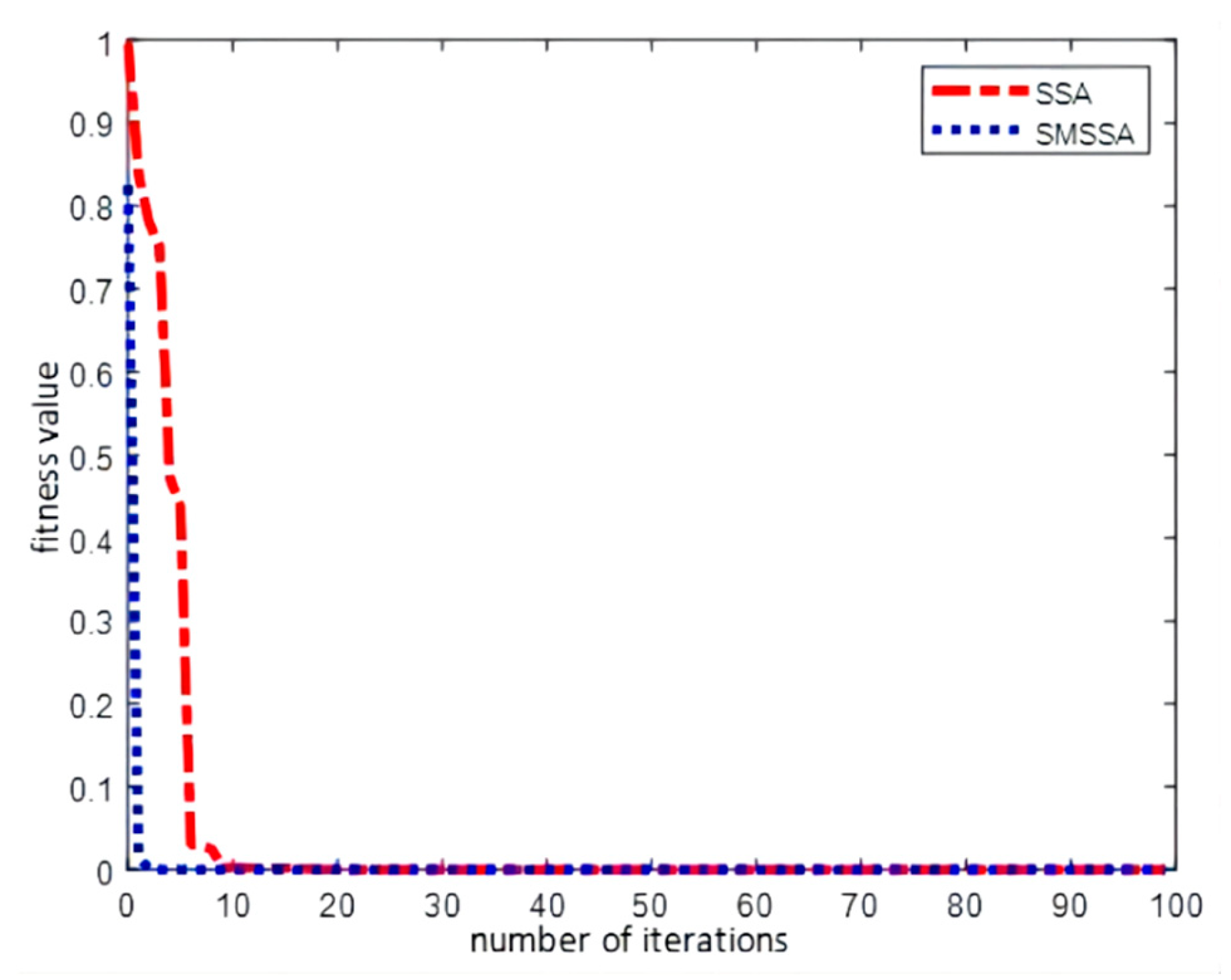
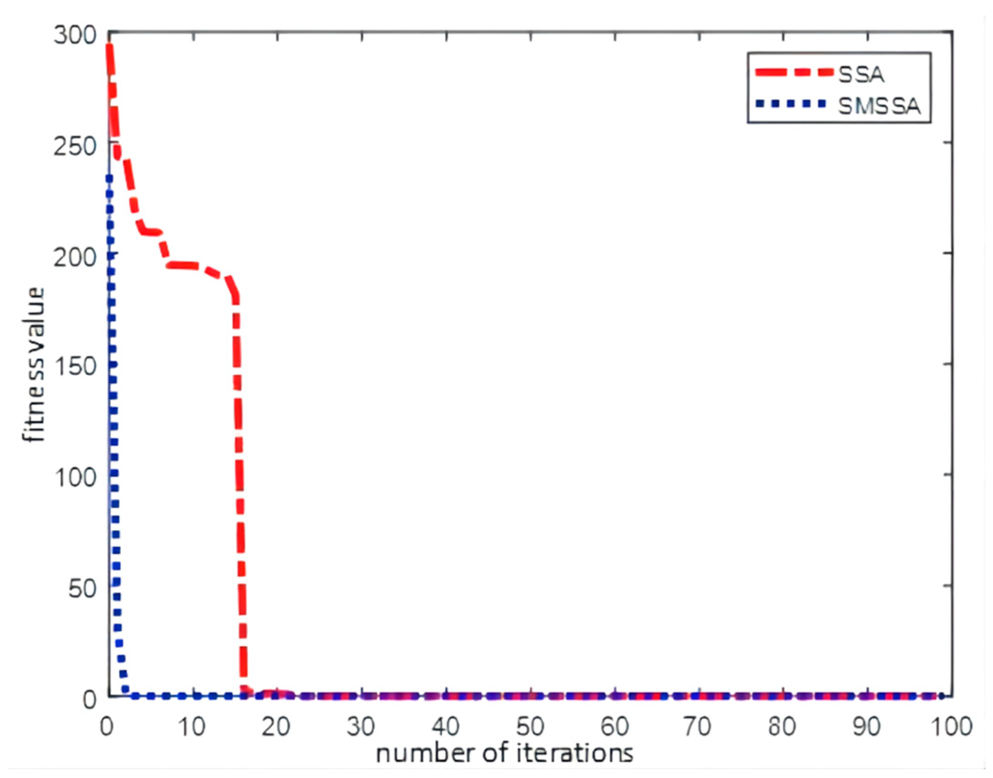
4.3. Improved Sparrow Search Algorithm Performance Test Simulation

The sparrow search algorithm and the modified sparrow search algorithm were described in the previous part, and in order to evaluate their optimization searching abilities, three typical benchmark test functions are selected in this section to test the performance of these two methods.

(1)

Test Functions

1.   Sphere function

$$f_1(x)=\sum _i^N{x}_i^2, x_i\in [-\mathrm{100,100}]$$

(17)

This function is a nonlinear symmetric single-peaked function with only one global extreme point, and the function achieves a global minimum $f_1\left(x\right)=0$ when x = $(\mathrm{0,0},\cdots ,0)$ This function allows for a test of the algorithm’s optimization-seeking accuracy.

2.   Griewank function

$$f_2\left(x\right)={\displaystyle \frac{1}{4000}}\sum _i^N{x}_i^2-\prod _i^{N}cos\left({\displaystyle \frac{x_i}{\sqrt{i}}}\right)+1, x_i\in [-\mathrm{600,600}]$$

(18)

This function contains a large number of local extremes over the entire range, and there exists a global minimum extreme value $f_2\left(0\right)=0$. The use of this function enables a test of the algorithm’s capacity to move beyond the local and continue the search.

3.   Rastrigin function

$$f_3(x)=\sum _i^N\left[x_i^2-10\mathit{cos}\left(2\pi x_i\right)+10\right], x_i\in [-\mathrm{5.12,5},12]$$

(19)

This function is a multi-peaked function with a large number of local extreme points, and at $x=(\mathrm{0,0},...,0)$, there is a global minimum point, and there is some difficulty in finding the global minimum point, so this function can be a test of the algorithm’s global optimization-seeking ability.

(2)

Comparison of algorithms

In order to assure the fairness of the algorithms and the control variables in this study, the size of the population is set at 30, and the highest possible number of iterations is set at $ite{r}_{max}$ for 100. Three test function parameter configurations are provided in

Table 1. Test function parameter settings.

Test Function	Dimension	Space Search	Target Value
Sphere	20	(−100, 100)	0.0
Griewank	20	(−600, 600)	0.0
Rastrigin	20	(−5.12, 5.12)	0.0

:

The results of testing SSA and SMSSA with the three test functions are shown in Figure 3, Figure 4 and Figure 5:

Figure 3, Figure 4 and Figure 5 show the performance curves of the two optimization techniques under the three test functions, from which it can be shown that the convergence speed of SMSSA is substantially quicker than that of SSA. To better assess the convergence outcomes of the two algorithms, the average and standard deviation of the two methods were calculated after each function is carried out 30 times, and the experimental findings are provided in

Table 2. Comparison of performance between SSA algorithm and SMSSA algorithm.

Test Function	Arithmetic	Theoretical Optimum	Average Value	Standard Deviation
Sphere	SSA	0	1.18 × 10−25	3.76 × 10−25
	SMSSA	0	6.23 × 10−34	3.19 × 10−34
Griewank	SSA	0	3.76 × 10−12	3.72 × 10−12
	SMSSA	0	7.22 × 10−15	6.38 × 10−15
Ristrigin	SSA	0	1.58 × 10−11	5.00 × 10−11
	SMSSA	0	3.29 × 10−13	1.28 × 10−13

.

Table 2 shows that the average SSA value in the sphere test function is 1.18 × 10⁻²⁵ while the average value of SMSSA is 6.23 × 10⁻³⁴, and compared to SSA, the accuracy of SMSSA is nine orders of magnitude greater. In the Griewank function, the average value of SSA is 3.76 × 10⁻¹², while the average value of SMSSA is 7.22 × 10⁻¹⁵, and at this time, SMSSA is three orders of magnitude more accurate than SSA; in the test of the Ristrigin function, SMSSA accuracy is two orders of magnitude better than SSA. From the above, it can be learned that SMSSA is better than SSA in searching ability. It shows that SMSSA is able to find function values that are closer to the optimal value during the optimization search, indicating that it has better optimization results

4.4. Construction of SMSSA-BiLSTM Models

According to the deep learning theory and the characteristics of the prediction model [23,24], the BiLSTM network model is optimized using the SMSSA method, which is largely separated into the following three phases:

(1)

Establish the BiLSTM network model’s structure, including how many nodes are in each input layer, how many layers are in the hidden layer, and how many nodes are in the output layer. The number of nodes in the hidden layer is obtained by utilizing an optimization algorithm to determine which is the best.

(2)

The SMSSA method is used to maximize the learning rate, number of trainings, and number of nodes in the BiLSTM network’s hidden layer.

(3)

The optimized model is used to estimate the real load and assess the performance of the model.

To analyze the advantages and drawbacks of the individual locations of SMSSA populations, this study employs the error between the output value of the BiLSTM model and the real value as the fitness function of the SMSSA algorithm. In this study, the MAE function is chosen as the fitness function of the algorithm, and the function formulation is given in the following Equation (20).

$$MAE={\displaystyle \frac{1}{n}}\sum _1^n\left|{\widehat{X}}_i-X_i\right|$$

(20)

where ${\widehat{X}}_i$ denotes the predicted value; $X_i$ denotes the true value; and n denotes the size of the population.

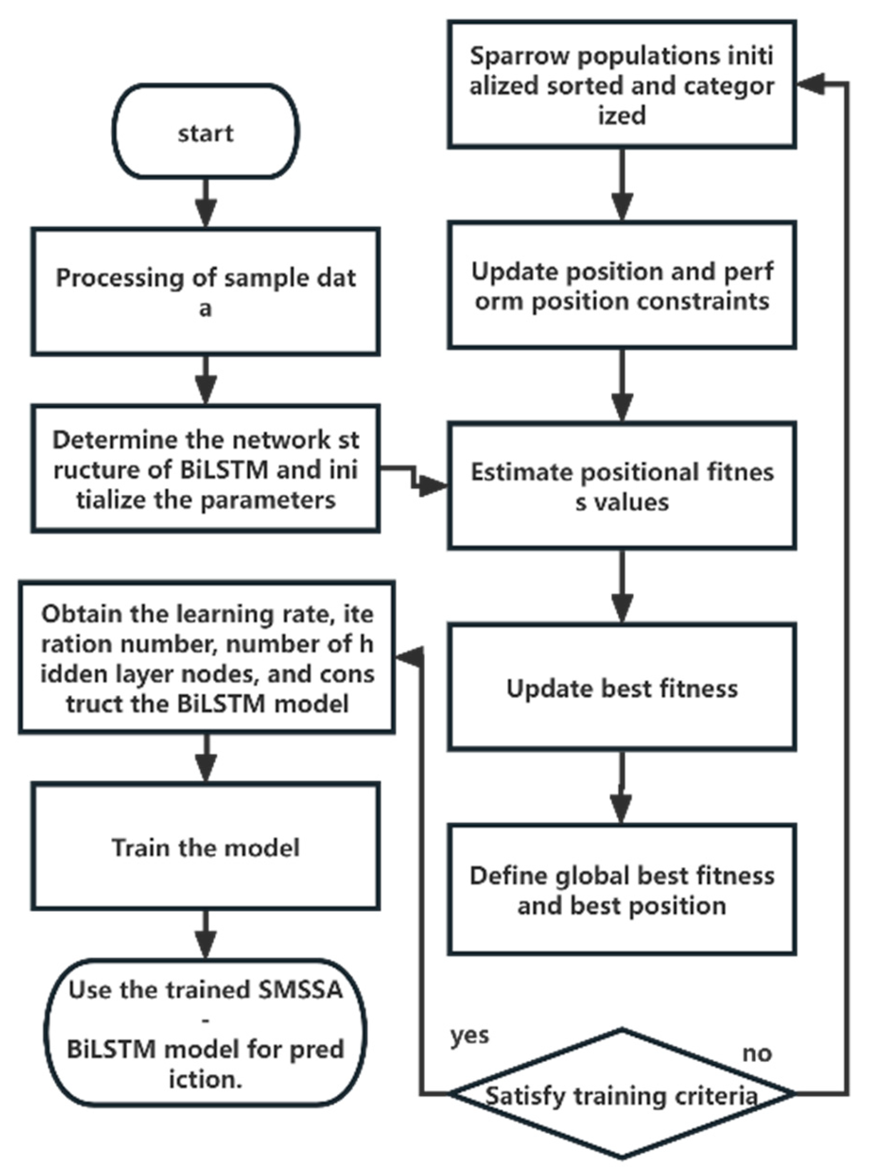
4.5. Prediction Process of SMSSA-BiLSTM Model

The specific steps and flowchart of the optimized BiLSTM network prediction model based on SMSSA algorithm are shown in Figure 6:

(1)

Determine the initial parameters of the model. Determine the sparrow population size N, the maximum number of iterations $T_{max}$, the upper bound ub and lower bound lb of the population search, the dimension d, and the proportion of discoverers P. Use a random function to determine the sparrow’s starting location. Count the number of nodes in the BiLSTM network’s input and output layers as well as the number of hidden layers.

(2)

Determine each sparrow’s specific adaptations and note where the best, worst, and suboptimal adaptations are found, $X_b$, $X_t$ and ${ X}_w$, as well as their adaptation values, $f_b$, $f_t$ and ${ f}_w$.

(3)

The sparrow’s position is updated by the finder, follower, and warning formulas, and the hyperparameters constrained by the boundary function are passed into the BiLSTM prediction model to return the adaptation values. Replaces are made if the current sparrow position’s ideal adaptation value is greater than the optimal position’s adaptation value; otherwise, nothing changes.

(4)

Determine if the algorithm has finished. If the number of iterations reaches the maximum number of iterations $T_{max}$ and model accuracy, output the location of the ideal population, feed the acquired parameters back to the BiLSTM prediction model, and predict the trained optimization model on the original data to obtain the result.

Figure 6. SMSSA-BiLSTM model prediction flow chart.

Figure 6. SMSSA-BiLSTM model prediction flow chart.

5. Simulation Analysis

In this study, the proposed SMSSA-BiLSTM short-term load forecasting model is verified using the real load data of the Wuxi region in Jiangsu Province, China in 2018. In this section, simulation analysis is carried out in three steps: firstly, the data and simulation environment required in the experiments in this section are determined; then, the example simulation of the established model is carried out; and finally, the performance effect of the model is compared and analyzed through the load curves, relative error plots, and the indicators such as RMSE, MAE, and MAPE.

5.1. Data Selection and Simulation Environment

(1)

Selection of data

In this article, the genuine electric load data of an area in 2018 is picked. The load data have a sample interval of fifteen minutes; that is, there are 4 sampling points in each hour, and a day comprises 96 sample points. Since the electric load has different change characteristics in different seasons, and the change characteristics of spring, fall, and winter are similar, they are taken as the first type of date; summer is the most special, and summer is taken as the second type of date. Therefore, in this section, the power load data from 1 March 2018, 0:00 to 31 March 2018, 24:00 in the region will be used as the first type of research object, which is used to describe the model’s prediction in the spring, fall, and winter, whereby the data collected before to 31 March serve as the training set, and the data collected on 31 March serve as the test set; the power load data from 1 July, 0:00 to 31 July are adopted as the second type of research object to describe the model’s prediction in summer, where the training set is the data collected before 31 July, and the test set is the data collected on 31 July.

(2)

Simulation environment

In this paper, MATLAB is chosen as the simulation environment, and the programming environment used is MATLAB version 2021a; the computer processor was Intel core i7 10875H, using a Windows 11 system.

(3)

Error evaluation metrics

To assess the superiority of this paper’s suggested SMSSA-BiLSTM model, the following three error evaluation metrics will be used to evaluate the model in this paper.

$$RMSE=\sqrt{{\displaystyle \frac{1}{n}}\sum _{i=1}^n{\left(y_i-{\widehat{y}}_i\right)}^2}$$

(21)

$$MAE={\displaystyle \frac{1}{n}}\sum _{i=1}^n\left|y_i-{\widehat{y}}_i\right|$$

(22)

$$MAPE={\displaystyle \frac{1}{n}}\sum _{i=1}^n{\displaystyle \frac{\left|y_i-{\widehat{y}}_i\right|}{y_i}}\times 100\%$$

(23)

where n is the sample capacity, $y_i$ is the value of the predicted output, and ${\widehat{y}}_i$ is the actual value.

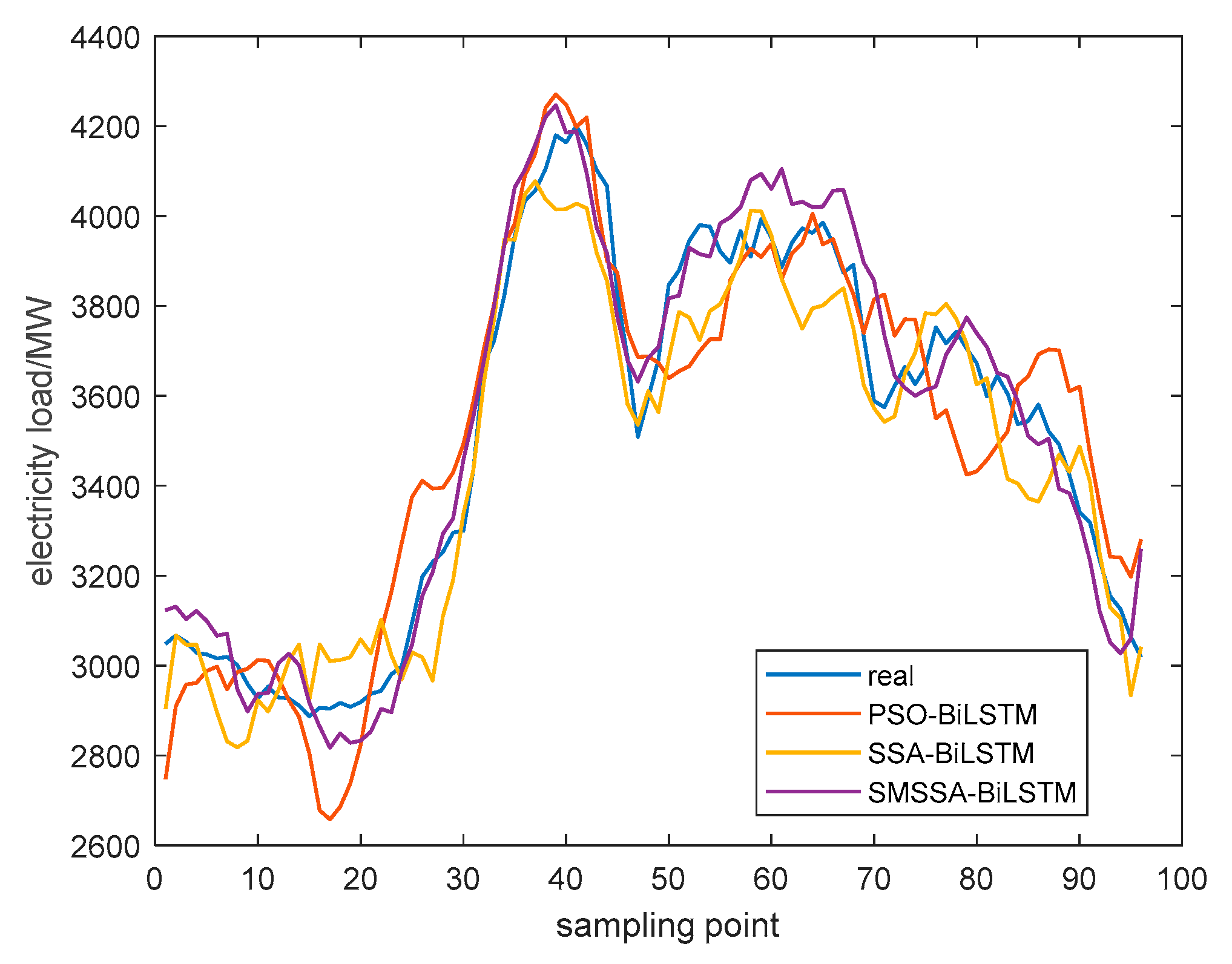
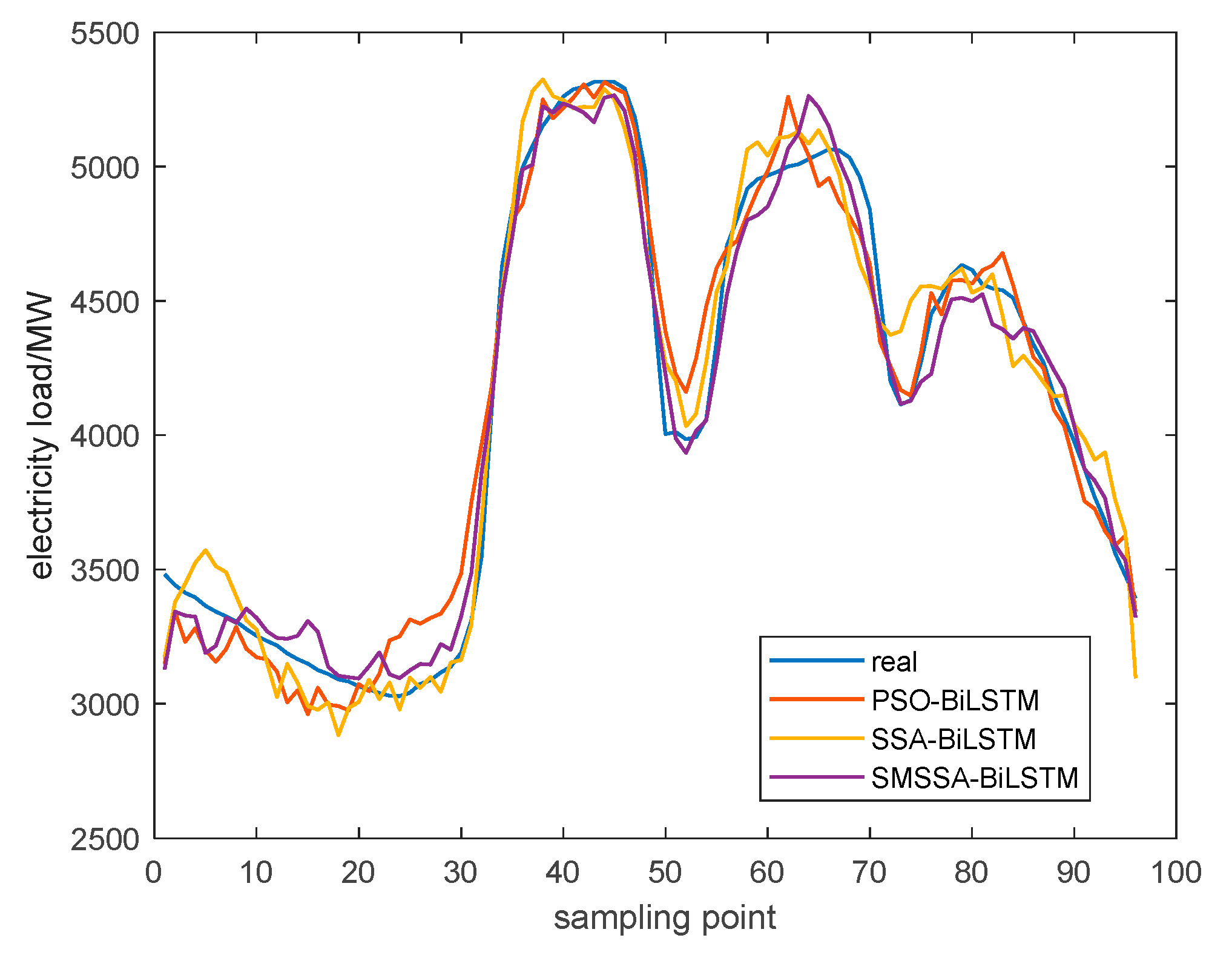
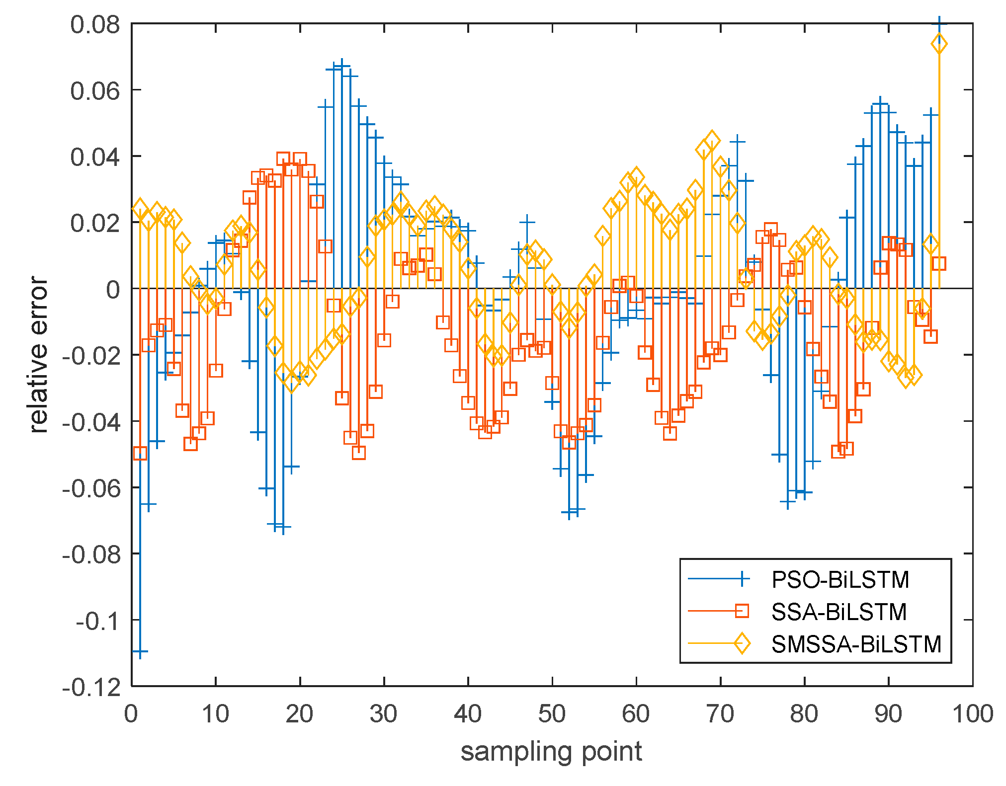
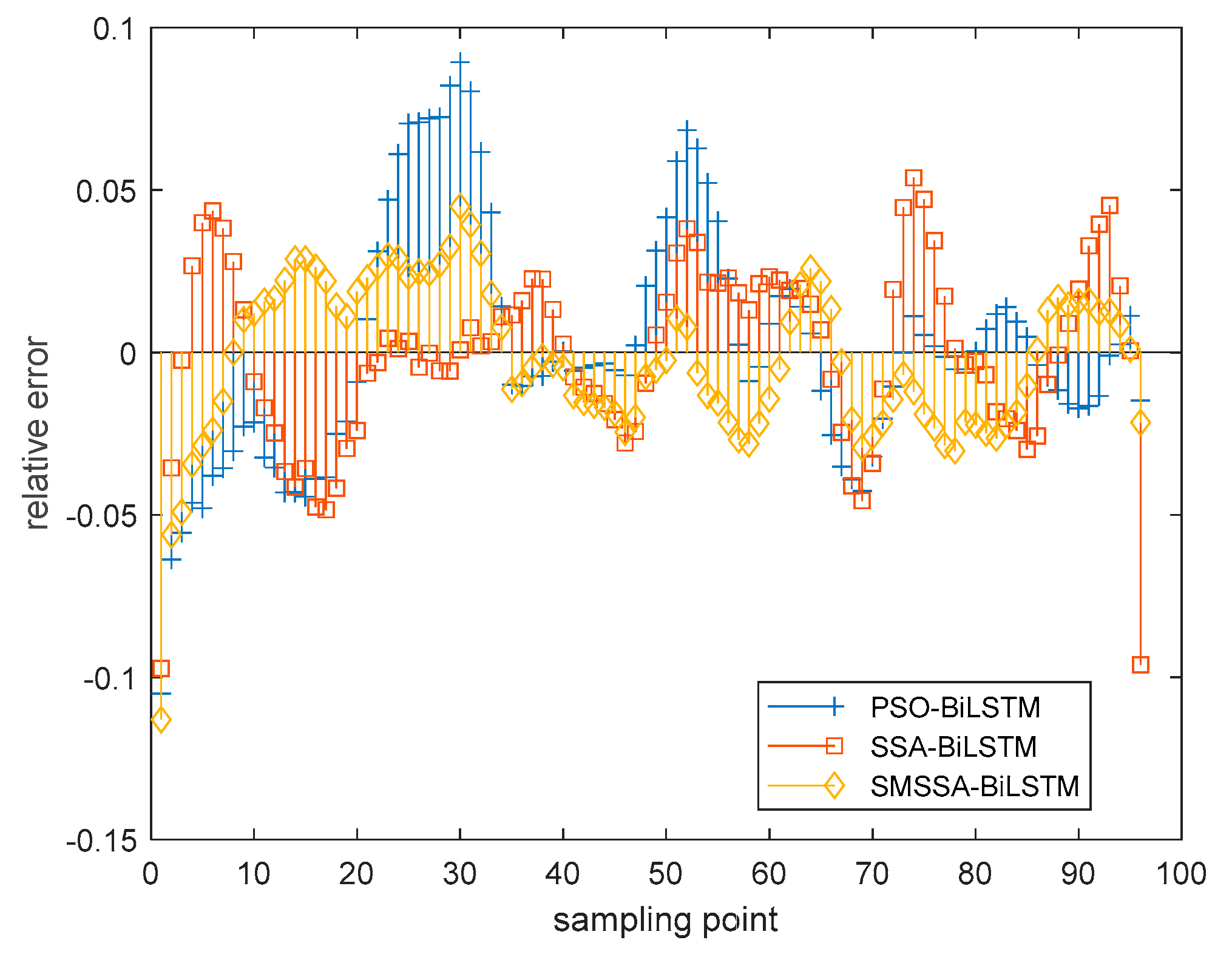
5.2. Simulation Process and Analysis

In this part, a multiple-input, multiple-output model is used to forecast the 96-load data of the following day using the 96-load data of the previous day and the highest and lowest temperature of the following day. The present study employs a BiLSTM model with two hidden layers. The number of nodes in hidden layer 1 is set to 200, and the number of nodes in hidden layer 2 is set to 20. The learning rate is set at 0.005. The model has 98 input nodes and 96 output nodes. The number of nodes of both hidden layers is set to [1, 300] for the search of optimization, the range of training times is set to [10, 300], the number of sparrow population is set to 5, the maximum number of iterations is set to 10, and the search of optimization for the learning rate is set to [0.01, 0.001]. In the SSA and SMSSA optimization algorithms, the warning value is set to 0.6, the proportion of discoverers is set to 0.7, the proportion of aware of dangerous sparrows is set to 0.2, and the worst number of sparrows for the simplex search in SMSSA is set to 5. The inertia weight in PSO is set to 0.8, and the learning factors are all set to 1.5. The following are the simulation results of each combined model.

The overlap between the real and projected values of many models, including SMSSA-BiLSTM, SSA-BiLSTM, and PSO-BiLSTM, is rated from high to low in Figure 7 and Figure 8. Due to the sparrow search algorithm’s advantage for the optimization time, the SSA-BiLSTM and SMSSA-BiLSTM load profiles fluctuate more than the PSO-BiLSTM load profiles and are smaller and more stable. In SMSSA-BiLSTM, the best-fitting results are obtained due to the stronger optimization seeking ability of the improved sparrow optimization algorithm. Further, their relative error curves are plotted as shown in Figure 9.

The relative errors of the three models for the first and second types of dates are displayed in Figure 9 and Figure 10, from which it is evident that the SMSSA-BiLSTM model has the highest forecast stability and the least amount of variation in relative errors, and most of its relative errors are concentrated near 2%, followed by the SSA-BiLSTM model, which performs a little bit poorer; the largest fluctuation of relative errors is that of the PSO-BiLSTM model, whose relative errors are more concentrated near 5%, which indicates that the prediction results of the SMSSA-BiLSTM model are more accurate.

Table 3. Predicted values of different load forecasting models.

Sampling Point	Actual Value (MW)	PSO-BiLSTM (MW)	SSA-BiLSTM (MW)	SMSSA-BiLSTM (MW)
1	3048	2747.11	2903.35	3123.14
2	3067	2909.45	3066.95	3131.26
3	3052	2958.33	3046.46	3103.63
4	3029	2961.12	3046.35	3121.46
5	3025	2988.31	2972.88	3099.32
6	3016	2997.53	2895.25	3066.20
7	3019	2947.23	2831.53	3070.89
8	3001	2985.50	2817.96	2947.12
9	2959	2992.92	2832.80	2897.79
10	2927	3012.80	2922.70	2936.87
11	2953	3010.87	2898.15	2939.44
12	2929	2972.52	2945.42	3005.58
13	2927	2922.96	3011.40	3026.32
14	2911	2886.00	3046.37	3001.41
15	2887	2804.23	2924.19	2917.03
16	2906	2678.05	3046.82	2864.42
17	2904	2657.74	3010.11	2817.48
18	2917	2686.11	3012.36	2849.18
19	2908	2737.43	3018.44	2828.40
20	2918	2821.99	3058.16	2832.48
21	2937	2954.65	3027.39	2852.91
22	2944	3076.14	3102.34	2903.58
23	2981	3164.35	3022.83	2896.01
24	2998	3272.54	2969.08	2988.25
25	3095	3374.65	3029.18	3046.53
26	3198	3411.10	3018.59	3155.55
27	3230	3393.57	2966.55	3207.54
28	3252	3395.72	3109.89	3293.16
29	3296	3430.21	3191.35	3327.88
30	3300	3493.47	3338.41	3458.48
31	3437	3588.89	3435.89	3555.30
32	3669	3704.28	3627.80	3677.18
33	3723	3803.90	3771.55	3800.62
34	3824	3935.53	3948.94	3936.64
35	3956	3982.81	3947.52	4063.60
36	4035	4090.46	4048.83	4103.73
37	4057	4139.46	4077.96	4159.73
38	4105	4241.07	4037.80	4220.50
39	4180	4271.11	4014.56	4246.69
40	4164	4248.36	4015.98	4186.14
41	4201	4198.59	4028.03	4188.56
42	4160	4220.04	4017.73	4096.38
43	4103	4035.01	3918.28	3974.41
44	4067	3901.14	3855.39	3917.36
45	3827	3874.28	3721.49	3776.09
46	3685	3744.66	3581.93	3679.55
47	3509	3686.84	3535.65	3632.12
48	3595	3688.05	3610.30	3684.94
49	3681	3673.98	3564.26	3709.10
50	3847	3639.41	3682.40	3817.39
51	3879	3655.12	3787.28	3823.51
52	3946	3666.19	3774.13	3929.55
53	3980	3699.21	3724.60	3915.93
54	3977	3726.61	3789.13	3910.37
55	3922	3726.48	3804.39	3984.26
56	3896	3857.93	3850.61	3997.45
57	3967	3897.54	3906.38	4019.75
58	3910	3927.59	4012.46	4080.65
59	3993	3909.16	4010.41	4093.94
60	3953	3938.80	3957.31	4060.62
61	3886	3860.73	3859.73	4104.93
62	3941	3917.16	3803.81	4027.03
63	3973	3940.04	3749.71	4032.20
64	3963	4004.98	3794.97	4019.75
65	3986	3937.14	3801.11	4021.05
66	3939	3949.48	3821.72	4057.08
67	3874	3880.77	3839.87	4058.12
68	3892	3825.82	3749.89	3982.33
69	3732	3740.79	3623.82	3896.62
70	3589	3814.75	3573.08	3857.26
71	3575	3826.02	3542.31	3734.95
72	3623	3734.69	3554.83	3645.18
73	3665	3770.85	3650.56	3618.00
74	3626	3769.68	3695.80	3600.15
75	3664	3665.84	3784.51	3613.52
76	3753	3550.13	3781.90	3620.93
77	3717	3568.19	3805.00	3692.27
78	3743	3495.66	3771.43	3729.30
79	3705	3424.45	3715.54	3775.04
80	3673	3432.33	3625.07	3739.84
81	3599	3457.64	3639.64	3709.07
82	3645	3490.29	3515.21	3651.94
83	3605	3521.31	3415.00	3642.90
84	3537	3623.05	3404.88	3587.46
85	3544	3643.25	3371.99	3510.71
86	3581	3692.53	3364.86	3492.24
87	3521	3703.73	3410.67	3504.95
88	3492	3701.34	3469.24	3393.38
89	3425	3610.68	3431.17	3383.56
90	3342	3620.40	3487.35	3323.01
91	3319	3472.42	3410.15	3233.84
92	3233	3354.25	3247.19	3119.12
93	3155	3242.35	3129.31	3051.70
94	3126	3240.47	3105.42	3027.70
95	3064	3198.01	2933.46	3059.66
96	3019	3280.52	3041.63	3259.66

shows the prediction values of the three models on 31 March in order to further quantify the prediction errors of each model.

Table 3 demonstrates the true and predicted values for 31 March at 15 min intervals. Various error evaluation metrics can be calculated from this table. To see the magnitude of every model inaccuracy, this paper uses the evaluation indexes RMSE, MAE, and MAPE to calculate the error, and various types of model errors are obtained, as shown in

Table 4. Comparison of prediction errors of different models.

	Errors	PSO-BiLSTM	SSA-BiLSTM	SMSSA-BiLSTM
first type	RMSE	147.7229	114.5868	90.1895
	MAE	121.1514	93.2343	74.3971
	MAPE	3.54%	2.72%	2.10%
second type	RMSE	156.6372	143.8687	115.0086
	MAE	119.8673	115.3176	92.1552
	MAPE	3.10%	2.85%	2.28%

.

As can be seen in Table 4, SMSSA-BiLSTM predicts the smallest MAPE values in both categories of dates. In the first category of dates, the MAPE of SMSSA-BiLSTM decreases by 1.44% and 0.62% compared to PSO-BiLSTM and SSA-BiLSTM, respectively; in the second category of dates, the MAPE of SMSSA-BiLSTM decreases by 0.82% and 0.57% compared to PSO-BiLSTM and SSA-BiLSTM, respectively. Comparing the results with the other two algorithms it can be demonstrated that SMSSA-BiLSTM can predict the ‘threshold’ more accurately.

6. Conclusions

This paper firstly introduces the bidirectional long- and short-term memory network (BiLSTM), which is an improvement of the long and short-term memory network (LSTM), which efficiently uses the backward information in addition to learning the ahead information, so it can fully learn the load data. Then, an enhanced sparrow search algorithm is presented, which primarily addresses algorithmic issues with the classical sparrow search algorithm’s population adaptation, search mechanism, and detection mechanism. It also addresses issues with the classical sparrow algorithm’s slow convergence speed and tendency to fall into local optimality. This serves as the foundation for the establishment of a short-term power load forecasting model that uses an improved sparrow search algorithm to optimize BiLSTM. The model compares its parameters, including the number of hidden layer nodes, learning rate, and training times, to those of SSA-BiLSTM and PSO-BiLSTM. Real load data from 2018 in Wuxi, Jiangsu Province, China, are chosen for example analysis in order to verify the prediction performance of the prediction model proposed in this paper. The results demonstrate the effectiveness of the SMSSA-BiLSTM model, with a small error and good fitting effect.

References

1. Wang, K.; Zhang, J.; Li, X.; Zhang, Y. Long-Term Power Load Forecasting Using LSTM-Informer with Ensemble Learning. Electronics 2023, 12, 2175. [Google Scholar] [CrossRef]
2. Li, J.; Lei, Y.; Yang, S. Mid-long term load forecasting model based on support vector machine optimized by improved sparrow search algorithm. Energy Rep. 2022, 8, 491–497. [Google Scholar] [CrossRef]
3. Ciechulski, T.; Osowski, S. High Precision LSTM Model for Short-Time Load Forecasting in Power Systems. Energies 2021, 11, 2983. [Google Scholar] [CrossRef]
4. Cui, C.; He, M.; Di, F.; Lu, Y.; Dai, Y.; Lv, F. Research on power load forecasting method based on LSTM model. In Proceedigns of the 2020 IEEE 5th Information Technology and Mechatronics Engineering Conference (ITOEC), Chongqing, China, 12–14 June 2020. [Google Scholar]
5. Butt, F.M.; Hussain, L.; Jafri, S.H.M.; Alshahrani, H.M.; Al-Wesabi, F.N.; Lone, K.J.; El Din, E.M.T.; Duhayyim, M.A. Intelligence based Accurate Medium and Long Term Load Forecasting System. Appl. Artif. Intell. 2022, 36, 2089. [Google Scholar] [CrossRef]
6. Jin, Y.; Guo, H.; Wang, J.; Song, A. A hybrid system based on LSTM for short-term power load forecasting. Energies 2020, 13, 6241. [Google Scholar] [CrossRef]
7. Kwon, B.; Park, R.; Song, K. Short-term load forecasting based on deep neural networks using LSTM layer. J. Electr. Eng. Technol. 2020, 15, 1501–1509. [Google Scholar] [CrossRef]
8. Rafi, S.H.; Masood, N.A.; Deeba, S.R.; Hossain, E. A short-term load forecasting method using integrated CNN and LSTM network. IEEE Access 2020, 9, 32436–32448. [Google Scholar] [CrossRef]
9. Chao, H.; Lin, F.; Pan, J.; Chien, W.; Lai, C. Power Load Forecasting Based on VMD and Attention-LSTM. In Proceedings of the 3rd International Conference on Data Science and Information Technology, Xiamen, China, 24–26 July 2020. [Google Scholar]
10. Yang, J.; Zhang, X.; Bao, Y. Short-term Load Forecasting of Central China based on DPSO-LSTM. In Proceedings of the 2021 IEEE 4th International Electrical and Energy Conference (CIEEC), Wuhan, China, 28–30 May 2021. [Google Scholar]
11. Siami-Namini, S.; Tavakoli, N.; Namin, A.S. The performance of LSTM and BiLSTM in forecasting time series. In Proceedings of the 2019 IEEE International Conference on Big Data (Big Data), Los Angeles, CA, USA, 9–12 December 2019. [Google Scholar]
12. Yan, L.; Zhang, H. A Variant Model Based on BiLSTM for Electricity Load Prediction. In Proceedings of the 2021 IEEE International Conference on Power, Intelligent Computing and Systems (ICPICS), Shenyang, China, 29–31 July 2021. [Google Scholar]
13. Wang, Z.; Jia, L.; Ren, C. Attention-Bidirectional LSTM Based Short Term Power Load Forecasting. In Proceedings of the 2021 Power System and Green Energy Conference (PSGEC), Shanghai, China, 20–22 August 2021. [Google Scholar]
14. Hochreiter, S.; Schmidhuber, J. Long short-term memory. Neural Comput. 1997, 9, 1735–1780. [Google Scholar] [CrossRef] [PubMed]
15. Graves, A. Connectionist temporal classification. In Supervised Sequence Labelling with Recurrent Neural Networks; Springer: Berlin/Heidelberg, Germany, 2012; pp. 61–93. [Google Scholar]
16. Wang, Y.; Sun, S.; Cai, Z. Daily Peak-Valley Electric-Load Forecasting Based on an SSA-LSTM-RF Algorithm. Energies 2023, 16, 7964. [Google Scholar] [CrossRef]
17. Zhong, B. Deep learning integration optimization of electric energy load forecasting and market price based on the ANN–LSTM–transformer method. Front. Energy Res. 2023, 11, 1292204. [Google Scholar] [CrossRef]
18. Liu, G.; Guo, J. Bidirectional LSTM with attention mechanism and convolutional layer for text classification. Neurocomputing 2019, 337, 325–338. [Google Scholar] [CrossRef]
19. Li, Z.; Hu, R.; Liu, X.; Deng, Y.; Tang, P.; Wang, Y. Multi-factor short-term load forecasting model based on PCA-DBILSTM. Proc. CSU-EPSA 2020, 32, 32–39. [Google Scholar]
20. Gong, P.; Luo, Y.; Fang, Z.; Dou, F. Short-term power load forecasting method based on Attention-BiLSTM-LSTM neural network. J. Comput. Appl. 2021, 41, 81–86. [Google Scholar]
21. Xue, J.; Shen, B. A novel swarm intelligence optimization approach: Sparrow search algorithm. Syst. Sci. Control Eng. 2020, 8, 22–34. [Google Scholar] [CrossRef]
22. Liu, C.; He, Q. Simplex-guided sparrow search algorithm with improved search mechanism. Comput. Eng. Sci. 2021, 44, 2238–2245. [Google Scholar]
23. Yaprakdal, F.; Arısoy, M.V. A Multivariate Time Series Analysis of Electrical Load Forecasting Based on a Hybrid Feature Selection Approach and Explainable Deep Learning. Appl. Sci. 2023, 13, 12946. [Google Scholar] [CrossRef]
24. Alghamdi, H.; Hafeez, G.; Ali, S.; Ullah, S.; Khan, M.I.; Murawwat, S.; Hua, L. An Integrated Model of Deep Learning and Heuristic Algorithm for Load Forecasting in Smart Grid. Mathematics 2023, 11, 4561. [Google Scholar] [CrossRef]
Figure 1. Structural diagram of long and short-term memory network. × denotes the Hadamard product and + denotes addition and recognizes the existence of explanations below.
Processes 12 01796 g001
Figure 2. BiLSTM structure diagram.
Processes 12 01796 g002
Figure 3. Iterative change diagram of sphere function.
Processes 12 01796 g003
Figure 4. Iterative change diagram of Griewank function.
Processes 12 01796 g004
Figure 5. Iterative change diagram of Rastrigin function.
Processes 12 01796 g005
Figure 7. Forecast results for 31 March.
Processes 12 01796 g007
Figure 8. Forecast results for 31 July.
Processes 12 01796 g008
Figure 9. Prediction errors of different network models on March 31st.
Processes 12 01796 g009
Figure 10. Prediction errors of different network models on July 31st.
Processes 12 01796 g010