A Hybrid Data-Driven and Model-Based Approach for Leak Reduction in Water Distribution Systems Using LQR and Genetic Algorithms

Abstract

This paper presents a pressure management technique for the reduction of leaks considering as a case study a branched water distribution system. The proposed technique is based on the detection and location of the leak using a genetic algorithm (GA) and pressure control using a Linear Quadratic Regulator (LQR). The validation of the proposed method uses measured pressure and flow data from a laboratory-scale water distribution system and its dynamic model.

1. Introduction

Leaks in water distribution systems (WDSs) cause significant resource losses and adverse economic impacts. Therefore, effective methods must be implemented to mitigate these leaks and ensure an adequate supply of water that meets consumer demands. In this sense, when a leak occurs in a WDS, it can affect the main intakes, causing the loss of large amounts of water. If the leak is visible and can be perceived through puddles on the surfaces, then, drilling work is performed to access and fix or change the damaged pipelines. On the other hand, when the leak cannot be identified on the surface, it becomes a critical task to locate and fix the leak before the losses become too elevated.

Water distribution pipeline networks are exposed to different factors that provoke leaks, such as deficient installations, corrosion, or wear, given the aging of the pipeline material, among others. Some of these factors can be prevented through maintenance operations; however, others are impossible to prevent due to their unpredictable nature, including illegal tapping, earthquakes, or the water-hammer effect that damages the joints between pipelines, among others. The fact that most pipeline networks extend underground makes maintenance, monitoring operations, and the visual identification of leak events more difficult [1]. Therefore, it is important to develop techniques to detect and promptly identify possible leaks and reduce the leak flows by controlling some valves in the WDS and avoiding excessive pressures in the system. These methods must be composed of a diagnostic element whose objective is to detect and locate the leak and a controller used to improve the supply of the demands during the day and reduce the leaked outflow. The controller is designed to control some actuators, such as pressure-reducing valves (PRVs), located in strategic areas of the network [2].

The literature review demonstrates that research has been focused on the solving of the problem of leak diagnosis from model-based and data-driven perspectives. From the data-driven perspective, different methods have been implemented to predict and/or estimate different variables in the context of hydraulic networks, for example, those based on the use of neural networks [3]. However, in recent years, data-driven methods, especially those that rely on meta-heuristics, have gained special interest because they demonstrate greater flexibility and precision than their model-based counterparts, especially when applied to large-scale and more complex systems [4]. These methods are not restricted to the search for a unique solution. Instead, they are considered global search algorithms where a solution space is explored to find satisfactory solutions. The use of meta-heuristics has gained interest in the leak diagnosis field, given their capacity to find optimal solutions in complex and dynamic environments such as complex networks of pipelines [5,6]. Typically, meta-heuristics methods estimate parameters in the hydraulic model that change under the appearance of leak events. By estimating these parameters, it is possible to know the actual size of the leakage and their location [7]. Similar research has also focused on the optimal placement of sensors in water distribution networks [6,8] or multi-leak diagnosis [5,9,10].

In this sense, meta-heuristic techniques are widely used in locating leaks in hydraulic networks; for instance, Mashhadi et al. [11] designed an analysis of flow and pressure data obtained from the EPANET 2.2 hydraulic simulation software for the location of water leaks in a WDS using machine learning methods such as artificial neural networks and logistic regression. Ares et al. [12] developed a multi-class vector machine classifier algorithm to locate the leakage region in conjunction with a topological differential evolution algorithm. Romero et al. [13] proposed an algorithm based on pressure and flow data through graph interpolation to detect and locate the leak region in a hydraulic network. Hu et al. [14] designed a data-driven leak diagnosis model using density-based spatial clustering of applications with noise (DBSCAN). Romero et al. [15] proposed a leak diagnosis system using pressure sensors and a GA optimization technique that considers network nodes with/without sensors. Shahhosseini et al. [10] designed a leak detection and reduction system by determining the leak coefficients of each node by analyzing data using GA and Nonlinear Programming (NLP).

As can be inferred, leak diagnosis methods are of primary importance in detecting and locating leaks. However, even if the leak is diagnosed, immediate maintenance is not always possible due to several factors, such as the location of the leak, cost, and civil work, among others. In this scenario, it is also important to design methods to reduce the leaked outflow by manipulating pressure-reducing valves without affecting the water supply until the leak can be properly fixed. Research has been reported in the state of the art for this problem, e.g., Galuppini et al. [16] designed a Proportional-Integral (PI) controller to control pressure and reduce leaks in a WDS. Ayad et al. [17] designed a water loss detection and pressure management system in a WDS using mathematical models and the GA. Dai et al. [18] developed a pressure reduction system to decrease the magnitude of water losses in a WDS by controlling a PRV using a nonlinear programming approach. Jones et al. [19] developed a study in a hydraulic network by locating PRVs through a WDS, demonstrating that in certain regions, such as upstream of a branch, water leaks can be avoided. Tian et al. [20] designed a method to control the pressure applied in the PRVs distributed throughout the WDS, using a greedy algorithm that determines the optimal control sequence for the valves.

As discussed above, detecting leaks and reducing water losses due to leaks are of primary importance in achieving satisfactory management of water distribution networks. Nonetheless, most of the reported works are just dedicated to solving these problems independently. Furthermore, most controllers are based on a model-based approach using classical control techniques such as Proportional-Integrative-Derivative (PID) or Linear Quadratic Regulator (LQR) controllers. Therefore, it is important to develop research that can hybridize both methodologies. This could have advantages for detecting leaks and controlling the pressure levels in the WDS more efficiently than considering only a model-based or data-driving method.

This work proposes a hybrid method to detect and reduce leak-flows in a WDS. The diagnostic method is a genetic algorithm-based technique for a network with two branches. The controller manipulates a pressure-reducing valve using a LQR in a critical node. The reduction of the leaks consists in identifying when a leak occurs during a time of minimum demand and then reducing the pressure using the PRV. If the leak occurs during times of maximum demand, the controller is not activated so as not to affect the critical demand areas of the hydraulic network. The method is validated by considering a water system with two branches located at the Technological Institute of Tuxtla Gutiérrez. It is important to emphasize that the proposed approach can be adapted to other topologies with more branches or a single pipeline like the one at the entrance point of a district-metered area.

This paper is structured as follows: Section 2 presents the main materials and methods used in the research. Section 2.1 presents the description of the proposed case study as well as the modeling of the system. Then, Section 2.2 presents the main ideas behind leak location using the GA and the design of the proposed controller. In Section 3, results of the proposed methodology are presented, and finally, Section 4 presents the discussion of the results and the conclusions of the paper.

2. Materials and Methods

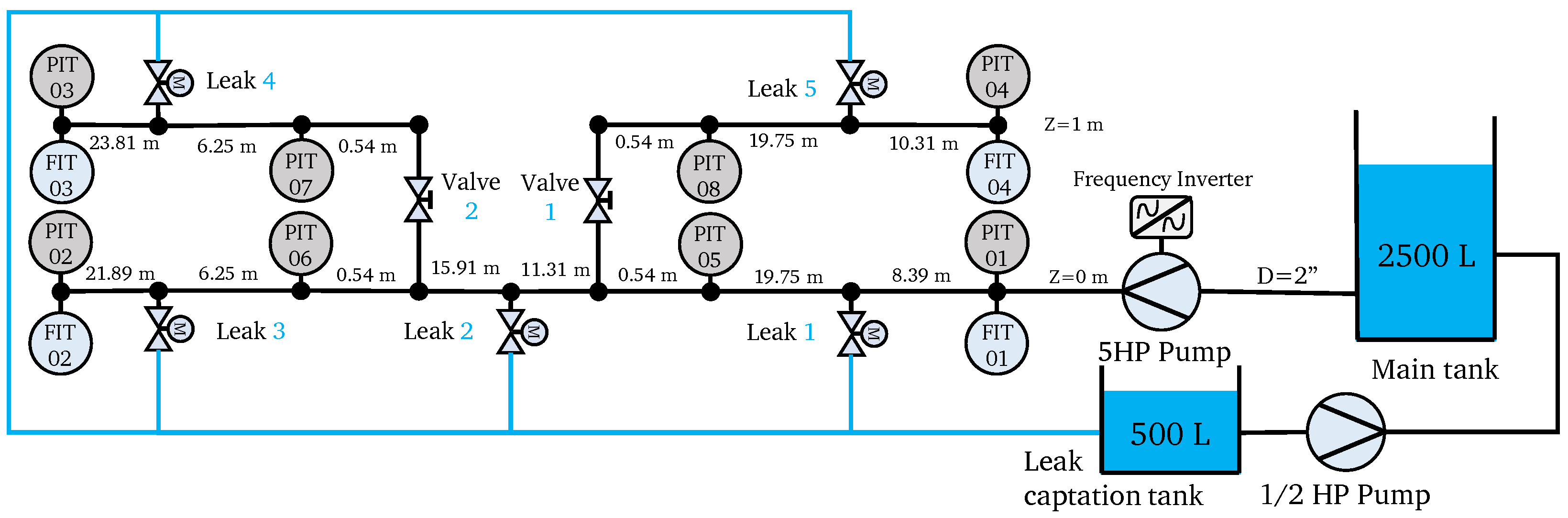
2.1. Case Study and Problem Formulation

The pilot plant considered in this paper is located at the Technological Institute of Tuxtla Gutierrez, Mexico and is displayed in Figure 1. The Pipeline and Instrumentation Diagram (P&ID) is displayed in Figure 2. It is a re-configurable plant that is controlled by two spherical valves located in the branches (see Figure 2), which can be configured as a single pipeline or a branched network. The WDS is fed with a reservoir with a capacity of 2500 L using an Evans 6IME0500 5hp centrifugal pump whose operating point can be varied using a frequency inverter, which allows the simulation of different flow input conditions. The system is instrumented with eight industrial Yokogawa EJA530E transmitters located in the nodes (PIT-1 to PIT-8), two Yokowaga ADMAG AXF magnetic flow meters located at the ends of the branches (FIT-3 and FIT-4), and two Yokogawa Rotomass Coriolis flow meters located at the input and the output of the main pipeline (FIT-1 and FIT-2). The acquisition of data is performed by a modular block (Yokogawa GM10) with five electronic valves (TONHE A20-T15-P2-B) to simulate leaks in different locations.

Figure 3 displays the schematic diagram of the hydraulic network with two branches, considering the variables that will be used to describe the dynamical model, the directions of the flows, the pressures in the nodes, and the control element: here, $z_i$’s [m] denotes the lengths of each section of the network, $Q_i$’s [m³/s] the flows through those sections, $H_i$’s [m] the pressures at the nodes, $H_{Bi}$’s [m] the pressures at the boundary nodes, $H_{\ell }$ the pressure at the leak, and $Q_{\ell }$ the leak flow (typically, $Q_{\ell }=\lambda \sqrt{H_{\ell }}$ for some leak coefficient $\lambda$ [m^5/2s⁻¹]). In addition, a pressure-reducing valve (PRV) is used as an actuator (generating $\Delta H_v$), and the main idea is to use a dynamical model for the whole system to design a controller acting on $H_2$, such that the leakage flow that occurs through the hydraulic network can be reduced.

The water-hammer equations explicitly consider transient pressure waves, allowing the system’s dynamic response to be accurately modeled. This dynamic representation is crucial for designing and evaluating the proposed LQR controller, which is based on a linearized model. By considering the water-hammer equations given in [21] and the finite differences approximation described in [22,23], the mathematical model that describes the flow through the hydraulic network is obtained as follows:

$$\begin{array}{cc}\hfill {\dot{Q}}_1\left(t\right)& ={\displaystyle \frac{{\beta }_1}{z_1}}\left(H_{B1}-H_2\right)+{\mu }_1\left(Q_1\right)Q_1\left|Q_1\right|-\Delta H_v,\hfill \end{array}$$

(1)

$$\begin{array}{cc}\hfill {\dot{H}}_2\left(t\right)& ={\displaystyle \frac{{\beta }_2}{z_1}}\left(Q_1-Q_2-Q_4\right),\hfill \end{array}$$

(2)

$$\begin{array}{cc}\hfill {\dot{Q}}_2\left(t\right)& ={\displaystyle \frac{{\beta }_1}{z_2}}\left(H_2-H_{\ell }\right)+{\mu }_2\left(Q_2\right)Q_2\left|Q_2\right|,\hfill \end{array}$$

(3)

$$\begin{array}{cc}\hfill {\dot{H}}_{\ell }\left(t\right)& ={\displaystyle \frac{{\beta }_2}{z_2}}(Q_2-Q_5-Q_3-Q_{\ell }),\hfill \end{array}$$

(4)

$$\begin{array}{cc}\hfill {\dot{Q}}_3\left(t\right)& ={\displaystyle \frac{{\beta }_1}{z_3}}\left(H_3-H_{B2}\right)+{\mu }_3\left(Q_3\right)Q_3\left|Q_3\right|,\hfill \end{array}$$

(5)

$$\begin{array}{cc}\hfill {\dot{Q}}_4\left(t\right)& ={\displaystyle \frac{{\beta }_1}{z_4}}\left(H_2-H_{B3}\right)+{\mu }_4\left(Q_4\right)Q_4\left|Q_4\right|,\hfill \end{array}$$

(6)

$$\begin{array}{cc}\hfill {\dot{Q}}_5\left(t\right)& ={\displaystyle \frac{{\beta }_1}{z_5}}\left(H_3-H_{B4}\right)+{\mu }_5\left(Q_5\right)Q_5\left|Q_5\right|.\hfill \end{array}$$

(7)

with

$${\beta }_1=g{A}_r,{\beta }_2={\displaystyle \frac{b^2}{g{A}_r}}.$$

(8)

where g is the acceleration of gravity [m/s²], $\nu$ is the kinematic viscosity [m²/s], $A_r$ represents the cross-sectional area of the pipeline [m²], b is the velocity [m/s] of the pressure wave, and finally, ${\mu }_i$ is a variable coefficient depending on the friction factor and, consequently, is a function of the flow rate $Q_i$, in the following form:

$${\mu }_i\left(Q_i\right)={\displaystyle \frac{-f\left(Q_i\right)}{2D{A}_r}},f\left(Q_i\right)={\displaystyle \frac{1.325}{{\left[ln\left(\frac{ϵ}{3.7d}+\frac{5.74}{{\left(\frac{4Q_i}{\pi d\nu }\right)}^{0.9}}\right)\right]}^2}},$$

with $f\left(Q_i\right)$ the Swamee–Jain friction factor, and $\Delta H_v$ the pressure variation due to the control element [24].

Here, a PRV is considered to regulate the pressure downstream in the WDS and reduce the leak. When the PRV is completely open, the outlet pressure is not reduced; otherwise, the outlet pressure can be reduced by manipulating the valve. The PRV is important because it prevents over-pressures in certain regions of the WDS that could fracture the pipelines. The equation that describes the behavior of a PRV is given by [25], and included in flow Equation (1) with term $\Delta H_v$ expressed as follows:

$$\Delta H_v=H_{v1}-H_{v2}={\displaystyle \frac{Q_1\left|Q_1\right|}{{\left(u_{v}E\right)}^2}},$$

(9)

where coefficient E represents the Torricelli factor $E=C_d{A}_d{\left(2g\right)}^{1/2}$, $C_d$ is the discharge coefficient, $A_d$ [m²] is the cross-sectional area of the orifice, and $u_v$ represents the shutter setting of the PRV, corresponding to the control variable. This valve directly controls pressure $H_2$ and will be used to control the pressure in the hydraulic network when water losses have been detected through leak diagnosis described in the following section.

2.2. Diagnosis and Control of Leaks

• Leak Location with Genetic Algorithms

As discussed above, the diagnosis element is performed using a GA, which is a meta-heuristic method inspired by the evolution of the species in which an iterative search of the fittest individual of a population is performed, thus providing an optimal solution to a provided problem. In the context of a GA, it is proposed that a population of candidate solutions for a given problem are found within a search area. The performance of each candidate solution is tested and those that provide the best performance are selected to create a new population similar to the best-performing individuals in the previous population. Using this iterative test and selection, the new population is iteratively enhanced until the fittest solution is found [26,27]. This process of performance testing and the creation of a new population takes place iteratively as the population gradually gets better at solving the problem until some termination criteria are met. A termination criterion can either be (1) a maximum number of generations (iterations) has already passed, or (2) an adequate solution was found such that the error is lower than a pre-set error value. This entire process is presented schematically in Figure 4.

In the case study considered in this paper, an EPANET model is used to generate simulated data for the operation of the hydraulic system. Real-world data for the leaking system are read from the pressure head and flow rate meters. Then, a simulation is performed using the EPANET model, which considers the same input conditions. Given that the simulation model does not contemplate the presence of a leak, it is not expected that the simulated and measured values will provide a satisfactory match. Thus, a genetic algorithm is implemented to calibrate an additional outflow ($\delta$) in some nodes suspected to present the leak. After the calibration, the $\delta$ value associated with the actual leaking node is expected to be significantly greater than zero. It is expected that after the calibration takes place, the $\delta$ value associated with the actual leaking node will be significantly greater than zero. In contrast, the other ones will be close to zero, meaning that no leak is detected at their corresponding nodes. For further information regarding the hydraulic model and parameters used to perform the hydraulic simulations, the reader is encouraged to consult reference [7].

For illustrative purposes, let us consider in Figure 5 a hypothetical scenario where a leak takes place at the second position (Leak 2 in Figure 2). The GA calibrates additional demand values in some nodes suspected of presenting the leak, minimizing the error between the measured and simulated values. The estimated demand for the node in which the leak actually occurs will evolve to values significantly higher than zero. In comparison, the estimated values for the rest of the nodes will tend to significantly lower values. The node in which the highest demand value is calibrated will be considered as the one with the leak. If no leak is detected, then, all values are calibrated to close-to-null values. An adequate threshold value must be manually implemented in such a way that those values that are calibrated above this threshold indicate the occurrence of a leak. It should be noted that even if the diagram represents a scenario where the leak takes place at the second position, the methodology can be generalized for leaks at other positions.

The location of the leak in the system was obtained through some experimental tests using a method based on the GA. The GA was set to run considering a lower search bound of 0 [$\mathrm{L}/\mathrm{s}]$ for all leak positions and an upper bound of $n\times {\delta }_{est}$ [$\mathrm{L}/\mathrm{s}]$, where ${\delta }_{est}$ is the latest estimation of the leaked outflow based on the latest inflow/outflow measurements, and n is a correction factor to account for the increase in the leak size over time. A population size of 100 individuals and a maximum number of generations of 20 were set considering a mutation function where the newly proposed solutions are adaptative concerning the last successful or unsuccessful generation. The mutation chooses a direction and step length that satisfies bounds and linear constraints. These parameters were selected because they adequately compromise execution time and valid identification. The GA was implemented in MATLAB R2022^® using the Global Optimization Toolbox, and any parameters not discussed here were considered their default values. In the experimental leak diagnosis tests, the system operated under a leak-free condition for a minute, and then, a leak was induced at some arbitrary location that was considered as unknown. This leak remained active during the rest of the experiment. The sampling period was 0.1 Hz. This sampling time is required due to the computational effort required by the GA. This high sampling time is enough to perform the leak diagnosis and control tasks and is congruent with real WDSs that work during long periods or 24/7 as discussed in [28].

The design of the control system to be used when a leak has been detected is described in the next subsection.

• Controller Design

Leak diagnosis using the GA locates the node where the leak occurs. A LQR controller is then designed to reduce the magnitude of water losses using a PRV located at the input node. LQR is a controller that calculates the optimal state feedback gain matrix K, with the aim of minimizing the performance index and obtaining the optimal input $u\left(t\right)$ to the system. Figure 6 displays the control system in a block diagram: the output signal $y\left(t\right)$, system state $x\left(t\right)$, and the feedback control with gains K, $K_I$ obtained from LQR design, are shown. It is important to mention that the error is integrated so that the output converges to the desired set point s (assumed to be provided by a manager according to the leak detection, as in [29]).

For the design of the LQR control system, the cost function is proposed in the following form:

$$J\stackrel{\mathrm{def}}{=}{\int }_0^{\infty }\left(x{\left(t\right)}^T\mathcal{Q}x\left(t\right)+u_v{\left(t\right)}^T\mathcal{R}{u}_v\left(t\right)\right)dt,$$

(10)

where $\mathcal{Q}$ and $\mathcal{R}$ are the weight matrices of appropriate dimensions, with $\mathcal{Q}={\mathcal{Q}}^T\ge 0$ and $\mathcal{R}={\mathcal{R}}^T>0$, and $u_v\left(t\right)=0$ when $t<0$. The LQR control is then the law $u_v\left(t\right)$ that minimizes the cost function J described in (10), under the dynamical constraint of system evolution of the form $\dot{x}\left(t\right)=A_{c}x\left(t\right)+B_{c}u\left(t\right)$ where u gathers all inputs of the system.

Matrices $A_c$, $B_c$ are calculated by means of approximate linearization of nonlinear model (1)–(7) around an equilibrium point, given here by $\overline{x}={[0.0030,1.99,0.0014,1.22,0.0007,0.0015,0.0007]}^T$ for $\overline{x}={[Q_1,H_2,Q_2,H_f,Q_3,Q_4,Q_5]}^T$ and for $\overline{u}={[H_{B1},H_{B2},H_{B3},H_{B4},\lambda ,u_v]}^T$, $\overline{u}={[5.6542,1,1,1,0,0.5]}^T$. The linearized matrices are given by

$$\begin{array}{cc}\hfill A_c& =\left[\begin{array}{ccccccc}{\alpha }_{11}& -{\displaystyle \frac{{\beta }_1}{z_1}}& 0& 0& 0& 0& 0\\ {\displaystyle \frac{{\beta }_2}{z_1}}& 0& -{\displaystyle \frac{{\beta }_2}{z_2}}& 0& 0& -{\displaystyle \frac{{\beta }_2}{z_1}}& 0\\ 0& {\displaystyle \frac{{\beta }_1}{z_2}}& {\alpha }_{33}& -{\displaystyle \frac{{\beta }_1}{z_2}}& 0& 0& 0\\ 0& 0& {\displaystyle \frac{{\beta }_2}{z_2}}& 0& -{\displaystyle \frac{{\beta }_2}{z_2}}& 0& -{\displaystyle \frac{{\beta }_2}{z_2}}\\ 0& 0& 0& {\displaystyle \frac{{\beta }_1}{z_3}}& {\alpha }_{55}& 0& 0\\ 0& {\displaystyle \frac{{\beta }_1}{z_4}}& 0& 0& 0& {\alpha }_{66}& 0\\ 0& 0& 0& {\displaystyle \frac{{\beta }_1}{z_5}}& 0& 0& {\alpha }_{77}\end{array}\right],\end{array}$$

$$\begin{array}{cc}\hfill B_c& =\left[\begin{array}{cccccc}{\displaystyle \frac{{\beta }_1}{z_1}}& 0& 0& 0& 0& {\displaystyle \frac{2g{A}_r{x}_1^2}{E^2{z}_1{r}^3}}\\ 0& 0& 0& 0& 0& 0\\ 0& 0& 0& 0& 0& 0\\ 0& 0& 0& 0& {\displaystyle \frac{-{\beta }_2\sqrt{H_3}}{z_1}}& 0\\ 0& {\displaystyle \frac{-{\beta }_1}{z_3}}& 0& 0& 0& 0\\ 0& 0& {\displaystyle \frac{-{\beta }_1}{z_4}}& 0& 0& 0\\ 0& 0& 0& {\displaystyle \frac{-{\beta }_1}{z_5}}& 0& 0\end{array}\right],\hfill \end{array}$$

with

$$\begin{array}{cc}\hfill {\alpha }_{11}=& 2|x_1|\mu \left(x_1\right)+{\displaystyle \frac{2\left(1.135\right)}{0.9\frac{5.74}{{\left(\frac{4}{\pi d\nu }\right)}^{0.9}}}}{\displaystyle \frac{{\left(x_1\right)}^{1.9}}{\ln {\left(\left(\frac{ϵ}{3.7d}\right)+\frac{5.74}{{\left(\frac{4x_1}{\pi d\nu }\right)}^{0.9}}\right)}^3}}-{\displaystyle \frac{2A_{r}g\left|x_1\right|}{z_1{E}^2{u}_v^2}},\hfill \\ \hfill {\alpha }_{33}=& 2|x_3|\mu \left(x_3\right)+{\displaystyle \frac{2\left(1.135\right)}{0.9\frac{5.74}{{\left(\frac{4}{\pi d\nu }\right)}^{0.9}}}}{\displaystyle \frac{{\left(x_3\right)}^{1.9}}{\ln {\left(\left(\frac{ϵ}{3.7d}\right)+\frac{5.74}{{\left(\frac{4x_3}{\pi d\nu }\right)}^{0.9}}\right)}^3}},\hfill \\ \hfill {\alpha }_{55}=& 2|x_5|\mu \left(x_5\right)+{\displaystyle \frac{2\left(1.135\right)}{0.9\frac{5.74}{{\left(\frac{4}{\pi d\nu }\right)}^{0.9}}}}{\displaystyle \frac{{\left(x_5\right)}^{1.9}}{\ln {\left(\left(\frac{ϵ}{3.7d}\right)+\frac{5.74}{{\left(\frac{4x_5}{\pi d\nu }\right)}^{0.9}}\right)}^3}},\hfill \\ \hfill {\alpha }_{66}=& 2|x_6|\mu \left(x_6\right)+{\displaystyle \frac{2\left(1.135\right)}{0.9\frac{5.74}{{\left(\frac{4}{\pi d\nu }\right)}^{0.9}}}}{\displaystyle \frac{{\left(x_6\right)}^{1.9}}{\ln {\left(\left(\frac{ϵ}{3.7d}\right)+\frac{5.74}{{\left(\frac{4x_6}{\pi d\nu }\right)}^{0.9}}\right)}^3}},\hfill \\ \hfill {\alpha }_{77}=& 2|x_7|\mu \left(x_7\right)+{\displaystyle \frac{2\left(1.135\right)}{0.9\frac{5.74}{{\left(\frac{4}{\pi d\nu }\right)}^{0.9}}}}{\displaystyle \frac{{\left(x_7\right)}^{1.9}}{\ln {\left(\left(\frac{ϵ}{3.7d}\right)+\frac{5.74}{{\left(\frac{4x_7}{\pi d\nu }\right)}^{0.9}}\right)}^3}}.\hfill \end{array}$$

where ${\alpha }_{11},{\alpha }_{33},{\alpha }_{55}\mathrm{and}{\alpha }_{77}$ come from the derivatives with respect to the flows. Notice that the control matrix, relating control variable $u_v$ to $\dot{x}$, reduces to the last one of $B_c$ (say b).

With the obtained matrices, it is possible to calculate feedback gains K and $K_I$ for the case study. By considering indeed the integrator as shown in Figure 6, an augmented model is obtained as follows:

$$\begin{array}{ccc}\hfill \left[\begin{array}{c}\dot{x}\left(t\right)\\ \dot{\xi }\left(t\right)\end{array}\right]& =& \left[\begin{array}{cc}{A}_c& 0\\ -C& 0\end{array}\right]\left[\begin{array}{c}x\\ \xi \end{array}\right]+\left[\begin{array}{c}{B}_c\\ 0\end{array}\right]u+\left[\begin{array}{c}0\\ 1\end{array}\right]s,\hfill \end{array}$$

(11)

$$\begin{array}{ccc}\hfill y\left(t\right)& =& \left[\begin{array}{cc}C& 0\end{array}\right]\left[\begin{array}{c}x\\ \xi \end{array}\right].\hfill \end{array}$$

(12)

for which a feedback gain can be obtained as

$$\begin{array}{cc}\hfill u_v\left(t\right)& =-Kx\left(t\right)+K_I\xi \left(t\right),\hfill \end{array}$$

(13)

$$\begin{array}{cc}\hfill \dot{\xi }& =s\left(t\right)-y\left(t\right)=s\left(t\right)-Cx\left(t\right),\hfill \end{array}$$

(14)

by resorting to standard LQR tools, for instance, from function lqr($A_a$,$b_a$,${\mathcal{Q}}_a$,$\mathcal{R}$) of Matlab© Control System Toolbox, where $A_a$, $b_a$ stand for augmented state and control matrices as in (11), ${\mathcal{Q}}_a$ is the state weight augmented accordingly, and $\mathcal{R}$ is the weight on $u_v$.

This control system is designed for the hydraulic network in conjunction with the leak diagnosis presented before. The next section presents some related application results.

3. Results

This section presents some results of the diagnosis and control system for leaks in the hydraulic network. Notice that, in the plant, the noise variance of the flow sensors is 2.53 × 10⁻¹⁰ m⁶/s², and the one for pressure sensors is 3.72 × 10⁻⁴ m². The weights used in the controller are $\mathcal{Q}=100I_d$ and $\mathcal{R}=20$. The initial pressure conditions in the hydraulic network are $H_{B1}\left(0\right)=5.6542$ m, $H_{B2}\left(0\right)=1$ m, $H_{B3}\left(0\right)=1$ m, $H_{B4}\left(0\right)=1$ m. The leak diagnosis simulation is carried out using the parameters presented in

Table 1. Parameters of the system.

Parameter	Value
Density of water, $\rho$	995.736 kg/m3
Kinematic viscosity, $\nu$	0.803 × 10−6 m2/s
Gravity acceleration, g	9.81 m/s2
Valve coefficient, $C_v$	1.156
Relative roughness, $ϵ$	0.347 × 10−4
Pipe diameter, d	0.048 m
Pressure wave velocity, c	422.754 m/s
Lenghts $z_1$ and $z_3$	38.94 m
Lenght $z_2$	31.056 m
Lenghts $z_4$ and $z_5$	38.94 m

.

The roughness coefficient of the pipeline was obtained in a previous investigation directly focused on calibrating the hydraulic model [30]. The pressure wave velocity was calculated according to the system’s characteristics, such as Young’s modulus of elasticity of the conduit walls, the density of the fluid, and the bulk modulus of elasticity [21]. The calculation of this parameter has been explicitly described in [31]. Note that these calculations were performed considering environmental temperature at approximately 30 C and the procedure described in [30]. The parameters must be recalibrated for different conditions.

Figure 7a–e present the result of the estimation of the leaked outflow for all the possible leak scenarios. During the first six time steps (that is, during the first 60 s = 1 min), the GA is able to identify the absence of the leak correctly. After the sixth time step, the calibrated leak rate value exceeds the manually selected threshold, causing the leak to be detected. The plots visually show the result provided by the GA. For each temporal step, a flow rate value is calibrated for each possible node, and the node with the highest flow rate is selected as the leaking result. As can be seen in Figure 7a–e, for each case, the estimated flow in the leaking node is significantly higher than the estimated flow for the rest of the suspicious nodes. Particularly in the case presented in Figure 7a, the values adjusted by the algorithm for nodes 2 to 5 are so low that they are practically null compared to the estimate for node 1. Similar results can be generalized in Figure 7b–e for the remaining leak scenarios. It is important to note that the stochastic nature of the GA can occasionally lead to instances where multiple nodes exhibit unexpectedly high leak flow estimates, as illustrated in Figure 7c. To mitigate this issue, incorporating additional constraints or heuristic rules within the GA could be explored to prioritize single-leak solutions. However, it is crucial to be aware that such modifications may compromise the algorithm’s ability to detect multiple simultaneous leaks, highlighting the trade-offs involved in the optimization process.

The leak diagnosis in the hydraulic network using the GA-based methodology allows us to obtain the location of the affected node. Then, the controller is activated to reduce the effect of the leak, that is, to ensure that an adjusted set-point is tracked [29]. Figure 8 shows a 24-h simulation, where the leak is detected at approximately 04:00 a.m.; the purple line at the top shows the leak-free demand, the blue dotted line corresponds to the pressure reduction (PR), that is, the new set-point when the leak was detected, the red line corresponds to the controlled pressure at the critical node successfully following the set reference, and finally, the yellow line represents the effect of pressure at the node where the leak occurs. The graph below shows the opening and closing of the pressure-reducing valve, where the adjustment of the set-point for the reduction in the pressure given the occurrence of the leak can be seen, and the valve closes 6% to generate the reduction effect of pressure throughout the system. Then, the PRV reopens to meet the reference set-point value. It can be emphasized that control actions in the network generate a $4\%$ decrease in the magnitude of the leak. It should be noted that even if this percentage was obtained using a small-sized experimental WDS in a laboratory context, the system here used as a case study was designed to replicate, as accurately as possible, the behavior of a large-scale urban WDS. Further testing of the proposed methodology in a more complex system and considering uncertainties in measured data or the system model needs to be conducted to obtain accurate performance metrics in a real-world implementation.

The reliability of the coupled LQR-GA approach was verified through a two-step process. First, the GA effectively identified the leak location by analyzing system node pressures. Subsequently, the LQR controller demonstrated its ability to reduce leak flow by regulating system pressures. To assess the robustness of the detection method, the leak diagnosis considered not only one but five different leak locations, obtaining satisfactory results, thus ensuring that the proposed method will perform satisfactorily for various leak scenarios. The control system proposed here demonstrates a solution for reducing water losses in WDS by compromising a trade-off between maintaining the water demand in the nodes and reducing the leak magnitude through the controller. This pressure management technique reduces the pressure in the system when the leak occurs, taking into account the hours of minimum demand for the reduction to avoid affecting the end users. This algorithm is not activated if the leak occurs during peak demand hours, given the importance of critical areas such as hospitals, industrial zones, and other institutions that must be supplied with enough water at all times.

4. Discussion and Conclusions

This paper introduces a hybrid method that integrates a data-driven GA for leak detection with a model-based pressure controller for a branched water distribution network. It should be noted that even if the application here demonstrated considers a branched WDS topology, similar results may still be obtained in a simpler topology (straight pipelines) or even in more complex ones (networks with loops). The GA estimates the size and location of the leak by measuring pressure and flow at critical nodes. Subsequently, an LQR controller is used to regulate the pressure at critical nodes of the WDS, aiming to minimize the leak. The proposed method has shown effective pressure management, preventing high-pressure levels in the node demands, reducing leak magnitudes, and minimizing water losses, achieving leak reductions of approximately 4%, which is a significant improvement given the prolonged duration of maintenance operations on real networks, which often result in substantial water losses. For instance, a system supplying 10,000 cubic meters of water daily could save approximately 146,000 cubic meters annually through a 4% reduction. This leads to substantial economic savings while contributing to environmental sustainability by conserving water and reducing energy consumption. The method demonstrates strong potential for practical implementation. However, further research is needed to address specific challenges and optimize performance for various system configurations.

References

1. Bohorquez, J.; Alexander, B.; Simpson, A.R.; Lambert, M.F. Leak Detection and Topology Identification in Pipelines Using Fluid Transients and Artificial Neural Networks. J. Water Resour. Plan. Manag. 2020, 146, 04020040. [Google Scholar] [CrossRef]
2. Khoa Bui, X.; Marlim, S.M.; Kang, D. Water network partitioning into district metered areas: A state-of-the-art review. Water 2020, 12, 1002. [Google Scholar] [CrossRef]
3. Peng, Y.; He, M.; Hu, F.; Mao, Z.; Huang, X.; Ding, J. Predictive Modeling of Flexible EHD Pumps using Kolmogorov-Arnold Networks. arXiv 2024, arXiv:2405.07488. [Google Scholar]
4. Quiñones-Grueiro, M.; Ares Milián, M.; Sánchez Rivero, M.; Silva Neto, A.J.; Llanes-Santiago, O. Robust leak localization in water distribution networks using computational intelligence. Neurocomputing 2021, 438, 195–208. [Google Scholar] [CrossRef]
5. Keramat, A.; Ahmadianfar, I.; Duan, H.F.; Hou, Q. Spectral transient-based multiple leakage identification in water pipelines: An efficient hybrid gradient-metaheuristic optimization. Expert Syst. Appl. 2023, 224, 120021. [Google Scholar] [CrossRef]
6. Yousefi-Khoshqalb, E.; Nikoo, M.R.; Gandomi, A.H. Chapter 14—Optimal deployment of sensors for leakage detection in water distribution systems using metaheuristics. In Comprehensive Metaheuristics; Mirjalili, S., Gandomi, A.H., Eds.; Academic Press: Cambridge, MA, USA, 2023; pp. 269–291. [Google Scholar] [CrossRef]
7. Gómez-Coronel, L.; Santos-Ruiz, I.; Torres, L.; López-Estrada, F.R.; Gómez-Peñate, S.; Escobar-Gómez, E. Digital Twin of a Hydraulic System with Leak Diagnosis Applications. Processes 2023, 11, 3009. [Google Scholar] [CrossRef]
8. Hu, Z.; Chen, W.; Chen, B.; Tan, D.; Zhang, Y.; Shen, D. Robust hierarchical sensor optimization placement method for leak detection in water distribution system. Water Resour. Manag. 2021, 35, 3995–4008. [Google Scholar] [CrossRef]
9. Rostami, I.; Darvishi, E. Combining inverse solution method and meta-heuristic algorithm to calculate the amount and location of leaks in water distribution networks. Irrig. Water Eng. 2021, 11, 87–104. [Google Scholar] [CrossRef]
10. Shahhosseini, A.; Najarchi, M.; Najafizadeh, M.M.; Hezaveh, M.M. Performance optimization of water distribution network using meta-heuristic algorithms from the perspective of leakage control and resiliency factor (case study: Tehran water distribution network, Iran). Results Eng. 2023, 20, 101603. [Google Scholar] [CrossRef]
11. Mashhadi, N.; Shahrour, I.; Attoue, N.; El Khattabi, J.; Aljer, A. Use of machine learning for leak detection and localization in water distribution systems. Smart Cities 2021, 4, 1293–1315. [Google Scholar] [CrossRef]
12. Ares-Milián, M.J.; Quiñones-Grueiro, M.; Verde, C.; Llanes-Santiago, O. A leak zone location approach in water distribution networks combining data-driven and model-based methods. Water 2021, 13, 2924. [Google Scholar] [CrossRef]
13. Romero-Ben, L.; Alves, D.; Blesa, J.; Cembrano, G.; Puig, V.; Duviella, E. Leak localization in water distribution networks using data-driven and model-based approaches. J. Water Resour. Plan. Manag. 2022, 148, 04022016. [Google Scholar] [CrossRef]
14. Hu, X.; Han, Y.; Yu, B.; Geng, Z.; Fan, J. Novel leakage detection and water loss management of urban water supply network using multiscale neural networks. J. Clean. Prod. 2021, 278, 123611. [Google Scholar] [CrossRef]
15. Romero-Ben, L.; Cembrano, G.; Puig, V.; Blesa, J. Model-free Sensor Placement for Water Distribution Networks using Genetic Algorithms and Clustering*. IFAC-PapersOnLine 2022, 55, 54–59. [Google Scholar] [CrossRef]
16. Galuppini, G.; Creaco, E.; Toffanin, C.; Magni, L. Service pressure regulation in water distribution networks. Control Eng. Pract. 2019, 86, 70–84. [Google Scholar] [CrossRef]
17. Ayad, A.; Khalifa, A.; Fawy, M.E.; Moawad, A. An integrated approach for non-revenue water reduction in water distribution networks based on field activities, optimisation, and GIS applications. Ain Shams Eng. J. 2021, 12, 3509–3520. [Google Scholar] [CrossRef]
18. Dai, P.D. Optimal pressure management in water distribution systems using an accurate pressure reducing valve model based complementarity constraints. Water 2021, 13, 825. [Google Scholar] [CrossRef]
19. Jones, F.T.; Barkdoll, B.D. Viability of pressure-reducing valves for Leak reduction in water distribution systems. Water Conserv. Sci. Eng. 2022, 7, 657–670. [Google Scholar] [CrossRef]
20. Tian, Y.; Gao, J.; Chen, J.; Xie, J.; Que, Q.; Munthali, R.M.; Zhang, T. Optimization of pressure management in water distribution systems based on pressure-reducing valve control: Evaluation and case study. Sustainability 2023, 15, 11086. [Google Scholar] [CrossRef]
21. Chaudhry, M.H. Applied Hydraulic Transients; Springer: Berlin/Heidelberg, Germany, 2014; Volume 415. [Google Scholar]
22. Henrie, M.; Carpenter, P.; Nicholas, R.E. Pipeline Leak Detection Handbook; Gulf Professional Publishing: Houston, TX, USA, 2016. [Google Scholar]
23. Tsetimi, J.; Mamadu, E.J. Finite Difference Analysis of Pressure Surge at the Valve of a Closed Pipeline. Int. J. Math. Trends Technol.-IJMTT 2022, 68, 22–35. [Google Scholar] [CrossRef]
24. Swamee, P.K.; Jain, A.K. Explicit Equations for Pipe-Flow Problems. J. Hydraul. Div. 1976, 102, 657–664. [Google Scholar] [CrossRef]
25. De Persis, C.; Kallesoe, C.S. Pressure regulation in nonlinear hydraulic networks by positive and quantized controls. IEEE Trans. Control. Syst. Technol. 2011, 19, 1371–1383. [Google Scholar] [CrossRef]
26. Mirjalili, S. Evolutionary Algorithms and Neural Networks: Theory and Applications, 1st ed.; Studies in Computational Intelligence; Springer: Berlin/Heidelberg, Germany, 2019; pp. 43–55. [Google Scholar] [CrossRef]
27. Katoch, S.; Chauhan, S.S.; Kumar, V. A review on genetic algorithm: Past, present, and future. Multimed. Tools Appl. 2021, 80, 8091–8126. [Google Scholar] [CrossRef]
28. Shao, Y.; Li, K.; Zhang, T.; Ao, W.; Chu, S. Pressure Sampling Design for Estimating Nodal Water Demand in Water Distribution Systems. Water Resour. Manag. 2024, 38, 1511–1527. [Google Scholar] [CrossRef]
29. Bermúdez, J.R.; López-Estrada, F.R.; Besançon, G.; Valencia-Palomo, G.; Santos-Ruiz, I. Predictive Control in Water Distribution Systems for Leak Reduction and Pressure Management via a Pressure Reducing Valve. Processes 2022, 10, 1355. [Google Scholar] [CrossRef]
30. Gómez-Coronel, L.; Santos-Ruiz, I.; Torres, L.; López-Estrada, F.; Delgado-Aguinaga, J. Model Calibration for a Hydraulic Network Using Genetic Algorithms. Mem. Congr. Nac. Control Automático 2022, 146–251. [Google Scholar] [CrossRef]
31. Bermúdez, J.; Santos-Ruiz, I.; López-Estrada, F.; Torres, L.; Puig, V. Diseño y modelado dinámico de una planta piloto para detección de fugas hidráulicas. In Proceedings of the Congreso Nacional de Control Automático CNCA, Monterrey, Mexico, 4–6 October 2017. [Google Scholar]
Figure 1. The hydraulic pilot plant at the Tuxtla Gutierrez Technological Institute.
Processes 12 01805 g001
Figure 2. The P&ID of the hydraulic pilot plant.
Processes 12 01805 g002
Figure 3. System of hydraulic network with two branches.
Processes 12 01805 g003
Figure 4. The GA as a flow chart.
Processes 12 01805 g004
Figure 5. Leak diagnosis methodology based on the GA for a hypothetical leak taking place in the second position.
Processes 12 01805 g005
Figure 6. Control diagram for reduction pressure.
Processes 12 01805 g006
Figure 7. Estimation of the leaked outflow for all the possible leak positions. (a) Estimation of the leaked outflow when a leak occurs at position 1. (b) Estimation of the leaked outflow when a leak occurs at position 2. (c) Estimation of the leaked outflow when a leak occurs at position 3. (d) Estimation of the leaked outflow when a leak occurs at position 4. (e) Estimation of the leaked outflow when a leak occurs at position 5.
Processes 12 01805 g007
Figure 8. Pressure control in the system according to the pressure profile for 24 h, with leakage effect.
Processes 12 01805 g008