Abstract
Severe ice accretion on transmission lines can disrupt electrical grids and compromise the stability of power systems. Consequently, precise prediction of ice coating on transmission lines is vital for guiding their operation and maintenance. Traditional single-model icing prediction methods often exhibit limited accuracy under varying environmental conditions and fail to yield highly accurate predictions. We propose a multi-scenario, two-stage adaptive ensemble strategy (MTAES) for ice coating prediction to address this issue. A combined clustering approach is employed to refine the division of ice weather scenarios, segmenting historical samples into multiple scenarios. Within each scenario, the bagging approach generates multiple training subsets, with the extreme learning machine (ELM) used to build diverse models. Subsequently, a two-stage adaptive weight allocation mechanism is introduced. This mechanism calculates the distance from the scenario cluster centers and the prediction error of similar samples in the validation set for each test sample. Weights are dynamically allocated based on these data, leading to the final output results through an adaptive ensemble from the base model repository. The experimental results show that the model is significantly better than traditional models in predicting ice thickness. Key indicators of RMSE, MAE, and reach 0.675, 0.522, and 83.2%, respectively, verifying the effectiveness of multi-scene partitioning and adaptive weighting methods in improving the accuracy of ice cover prediction.
1. Introduction
Ice formation on transmission lines is a common natural phenomenon. With the expansion of power grid infrastructure, more transmission lines are inevitably passing through regions susceptible to repeated icing due to geographical and climatic conditions [1]. This ice accretion poses a significant threat to the stability of power grids, often disrupting daily life and industrial production, leading to substantial economic losses [2,3]. Therefore, developing an accurate and effective model for predicting ice accretion on transmission lines is essential to mitigate these challenges.
Extensive research has been conducted on predictive models for ice coating on power grids, generally categorized into two main approaches: physical process-based models and data-driven models [4]. Physical process-based models, derived from ice formation mechanisms on overhead transmission lines, utilize hydrodynamic and thermodynamic principles to establish accurate growth models. Notable methodologies have been introduced by researchers such as Jones [5], Makkonen [6], and Lenhard [7]. However, the formation of ice coating is a complex, nonlinear process influenced by numerous factors, making these physical-process-based methods computationally intensive and often insufficient to capture the dynamics of ice formation [8,9] fully.
With the rapid development of big data and machine learning technologies [10,11], researchers have advanced data-driven predictive modeling studies. These studies predominantly utilize historical ice coating data, employing machine learning techniques to delineate the characteristics of nonlinear relationships, temporal dynamics, and uncertainty within the data. Refs. [12,13,14] model the relationship between ice coating thickness and various factors such as micro-meteorological conditions, microtopography, and other relevant variables to construct predictive models for ice coating on transmission lines. Ref. [15] segments the ice coating period into several stages and employs the Bat Algorithm (BA) to optimize input weights and bias thresholds in an extreme learning machine (ELM) for predicting ice coating thickness. Ref. [16] identifies air temperature, humidity, and ice coating reference data, highly correlated with transmission line ice coating, as input data, and ice coating quality as model output, proposing three models for ultra-short-term prediction, short-term hysteresis prediction, and rolling prediction based on the support vector machine algorithm. Ref. [17] develops effective fuzzy rules from ice coating monitoring data and establishes a comprehensive prediction model integrating fuzzy logic and neural networks. Ref. [18] introduces a multicore correlation vector machine optimized using the adaptive parallel Jaya (APJA) algorithm to model the growth rate of ice coating, incorporating the time accumulation effect in predicting ice coating thickness, and proposes a model considering this factor. Ref. [19] enhances a support vector machine regression model with similarity weighting and adjusts parameters through particle swarm and ant colony optimization algorithms to improve model generalization. Ref. [20] establishes a regression model for conductor ice coating based on the support vector machine. Ref. [21] extracts crucial micro-meteorological data through principal component analysis (PCA) and applies a genetic optimization algorithm to establish an efficient LS-SVM ice coating prediction model.
Despite the advancements in machine learning techniques for ice coating prediction, existing models often struggle with generalization across diverse meteorological conditions. For instance, while the support vector machine-based models provide reasonable predictions under specific conditions, their accuracy and stability are significantly affected by the selection of feature parameters, leading to reduced performance in varying climatic environments [22]. Similarly, models relying on single-line data may perform well within a localized context but fail to maintain accuracy when applied to different geographic or meteorological contexts [23,24]. These limitations highlight the need for a more robust and adaptable predictive model.
To address these challenges, the MTAES method introduced in this paper offers a novel approach by integrating multi-scenario adaptive ensemble prediction strategies. This method enhances the model’s ability to adapt to different environmental conditions, providing more accurate and reliable predictions of ice coating thickness across various microtopographic scenarios. The main contributions of this paper are as follows:
- To make more detailed and accurate predictions of ice cover thickness under different meteorological scenarios, we propose a method to classify these scenarios using the M-H-K combination algorithm. This method automatically determines the optimal number of clusters, enabling a more accurate and rational categorization of meteorological conditions affected by ice coating.
- Recognizing the importance of both high accuracy and diversity in base models for a high-performance ensemble, we implemented a bootstrapping approach to generate multiple different sample subsets. Each subset was used to train a base model using ELM. This approach ensures that the base models exhibit significant differences, thereby increasing the diversity and robustness of the overall ensemble model. This diversity is crucial for improving the adaptive weighted integrated prediction of ice coating thickness.
- To achieve high-precision ensemble performance, we designed a two-layer adaptive weight optimization mechanism. For each test sample, we calculated the distance to the scenario cluster center and the prediction error of similar samples in the validation set. Using similarity criteria, we converted these metrics into weights and combined them with the outputs of the base models to obtain the final prediction. This method helped accurately reflect the impact of meteorological and topographical features on ice thickness in different scenarios.
The remainder of this paper is organized as follows: Section 2 presents the construction of multi-meteorological scenarios for ice coating prediction. Section 3 discusses the strategy for generating diverse base models. Section 4 explores the enhanced weighting strategy for the adaptive ensemble model. Experiments are conducted in Section 5, and conclusions are drawn in Section 6.
2. Construction of Ice Coating Multi-Meteorological Scenarios
With increasing demands for a deeper consideration of meteorological conditions and terrain features, detailed and accurate prediction of ice coating thickness across various microtopographic scenarios is crucial for enhancing the adaptability and accuracy of the entire system. This section investigates the multi-scenario construction for the active prediction of ice coating thickness in depth.
2.1. Icing Meteorological Scenario Division Based on M-H-K
Traditional clustering methods, such as K-means [25], often face challenges when applied to ice coating scenario delineation. Specifically, K-means requires a predefined number of clusters, making it difficult to determine the optimal number of scenarios accurately. Additionally, the random selection of initial clustering centers can lead to instability and less reliable clustering results.
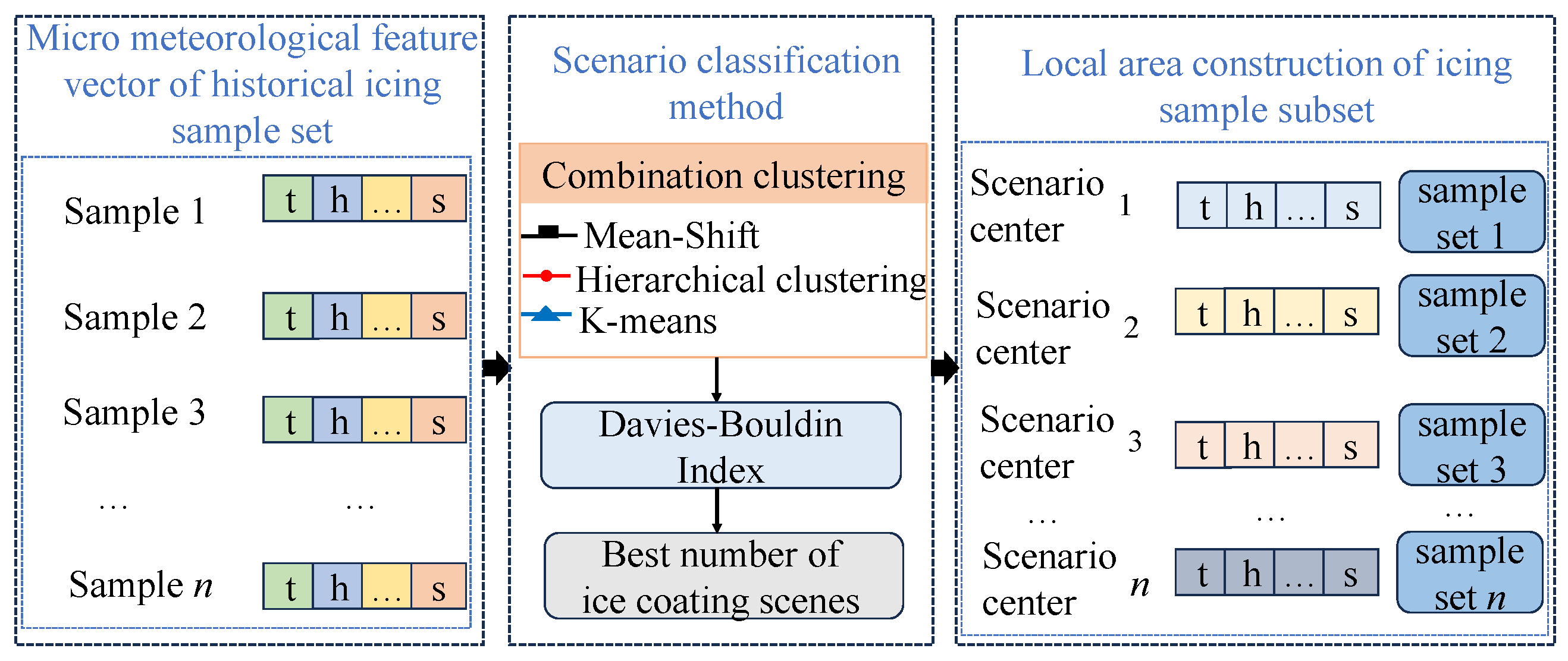
To address these issues, we propose a novel clustering algorithm, M-H-K, which integrates three distinct techniques. First, mean-shift (MS) identifies clustering centers based on the density distribution of the data [26], thereby avoiding the randomness associated with traditional methods and providing more reliable initial cluster centers. Second, hierarchical clustering (HL) combines the initial centers determined by MS to form an appropriate number of clusters [27], allowing for the dynamic determination of cluster numbers through the merging of similar clusters. Finally, K-means refines the clusters identified by MS and HL, enhancing the stability and accuracy of the clustering results through iterative adjustments. Figure 1 shows the schematic diagram of the classification of the ice coating scenarios, where t represents the temperature feature, h represents the humidity feature, and s represents the wind speed feature. The specific process of the integrated clustering method is shown in Figure 2, and its specific division process is as follows:
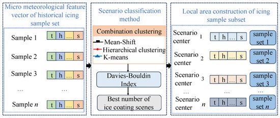
Figure 1.
Schematic diagram of ice coating scenario classification method.
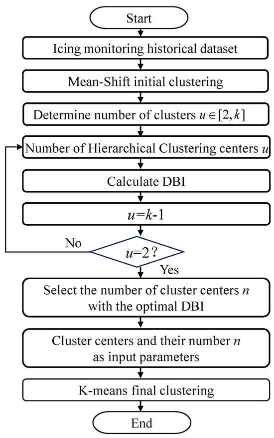
Figure 2.
Process of ice coating scenario division based on M−H−K.
- Determine initial clustering centers: For a historical training set , where N represents the total number of data points in the historical training set, the initial clustering centers are first determined using mean-shift clustering. Mean-shift identifies centers based on the density distribution of the data, avoiding the randomness typically associated with the initial selection of centers in other clustering methods. This density-based approach ensures that clustering centers are located in regions with a high concentration of data points. As a result, k clustering centers are obtained.
- Merge initial clustering centers: The initial clustering centers obtained in the previous step are merged using hierarchical clustering, resulting in a suitable range of cluster numbers, where each center represents a distinct cluster.
- Evaluate clustering: Calculate the Davies–Bouldin Index (DBI) for different numbers of cluster centers. This index is used as a clustering assessment metric for ice-covered scenarios, measuring both the compactness within clusters and the separation between them.
- Determine optimal number of clusters: The number of clusters corresponding to the lowest DBI value is selected as the optimal number of clusters. At this point, the merged cluster centers are determined, where n represents the optimal number of clusters.
- Final clustering with K-means: The optimal number of cluster centers u and the corresponding cluster centers are used as input parameters for K-means, which performs the final clustering of the dataset.
- Obtain final meteorological scenarios: Finally, the number of meteorological scenarios and their center points are determined based on the dataset.
2.2. Effectiveness Indicators for Scenario Division
The Davies–Bouldin Index (DBI) is a commonly used metric to assess the quality of clustering results. It measures the closeness within clusters and the separation between clusters by calculating the average distance between different clusters and the average distance between data points within clusters [28]. In practice, a smaller DBI indicates a better clustering effect because smaller intra-cluster distances and larger inter-cluster distances imply better-quality clustering results. The calculation of DBI is relatively simple, and its value has a small range of variation, so it is suitable as an indicator of the validity of clustering for ice-covered scenarios. Its calculation formula is as follows:
where k is the number of clusters, and and denote the average distance from each sample to the center of each cluster in categories i and j, respectively. denotes the distance between the centers of clusters of categories i and j.
3. Generation Strategy of Diversity Base Models
This section investigates the construction of diverse base models in multiple scenarios. Constructing a base model under each scenario is designed as an independent problem, and the base learners in the bagging-based ensemble learning approach are independent of each other without dependencies and can efficiently construct stronger learner models through parallel training [29], so this chapter obtains multiple subsets of different samples with the help of the bagging ensemble idea and utilizes an ELM on each subset to train a base model. These base models are somewhat different, thus increasing the diversity of the overall model.
3.1. Mechanism for Generating Diverse Subsets
It is well known that, to build a high-performance ensemble model, the base model must have high accuracy and diversity [30], and diversity refers to the existence of differences among base models, which is crucial in ensemble learning. In this section, a popular strategy, the stochastic subspace method, is used to construct subspaces, and the next section will detail how to construct a subset of the icing monitoring data from multiple scenarios for better subsequent building of diverse base models.
After dividing the multi-scenarios of ice coating, in order to make the individual models different from each other, this chapter starts from the perspective of manipulating the input features with the help of the idea of the ensemble strategy of bagging, which is a commonly used ensemble learning method and consists of bootstrap and aggregating. Bootstrap refers to the method of putative sampling, which is a putative back-sampling method, which constructs a different sub-dataset for each weak learner to train by sampling the original dataset with putback [31]. Aggregating refers to the strategy of combining the outputs of multiple weak learners. For the bagging algorithm, a number of sample subsets obtained can be considered independent of each other and do not interfere with each other so that the training of multiple base models can be run side by side at the same time, which speeds up the training speed of the model to a certain extent, and is good at improving the stability of the model that is very sensitive to small changes in the training set, and, at the same time, the sample subsets of the various scenarios are obtained by random sampling, which can enhance the generalization ability of the prediction model and effectively reduce the variance of the prediction model.
Given a training sample , the bootstrap resampling mechanism is used to perform multiple rounds of random sampling with replacement, extracting training data subsets of the same size from the dataset. Each subset contains about 60% of the independent samples from the original training set. This process is mathematically represented by the following formula:
3.2. Extreme Learning Machine
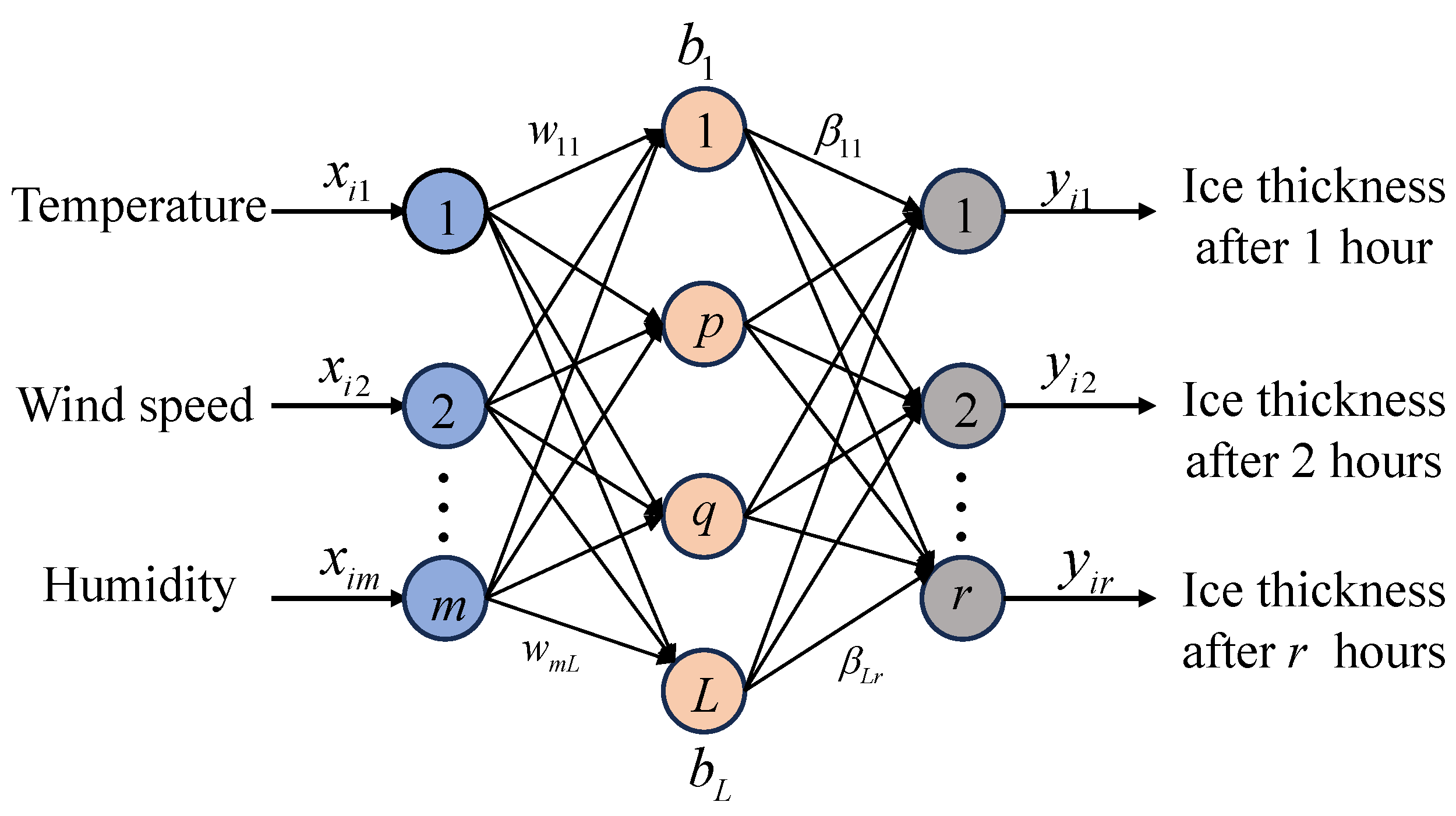
ELM is a learning algorithm for Single Hidden Layer Feedforward Neural Networks (SLFNs), proposed by Huang [32]. Numerous studies have demonstrated that ELM possesses a robust capacity for learning representations, boasting rapid learning speeds and strong generalization abilities [33,34]. Structurally, the ELM is a three-layer neural network comprising input, hidden, and output layers connected through a fully integrated architecture. Figure 3 illustrates its network structure. In this article, the input is meteorological features, and the output is ice thickness under different prediction durations. The core concept behind ELM involves utilizing a large-scale matrix of randomly generated neurons in the hidden layer to map input samples swiftly. The network adjusts the weights through a linear output layer to derive the final output. This random initialization process eschews the need for parameter tuning, significantly accelerating the training phase. Unlike traditional Back Propagation (BP) neural networks, ELM assigns initial weights to the hidden layer randomly and keeps them unchanged throughout the optimization process, focusing only on calculating the output variable weights during learning [35]. This unique approach reduces training times and enhances ELM’s capability to handle complex nonlinear processes and time-varying characteristics, making it well suited for predicting variations in ice coating thickness.
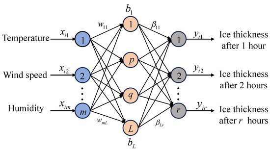
Figure 3.
Schematic of ELM.
The computational process is as follows: A set of ice data samples, , is given, where represents the ith ice accretion dataset input vector, and L is the number of nodes in the hidden layer, with m and r being the number of nodes in the input and output layers, respectively. The input–output relationship of the ELM is expressed by the following formula:
where i indicates the index of historical ice samples, is the weight vector connecting the jth hidden layer to the output layer, is the weight vector between the input layer and the jth hidden layer, represents the bias for the hidden layer, and is the activation function. denotes the output of the jth neuron in the hidden layer for . In this paper, the sigmoid function is used as the activation function, which is expressed as
During the learning process in an E network, the goal is to minimize the error in the output. The cost function is generally expressed as
It implies that there exist , , and , such that
We express the above equation in matrix form as
where represents the output weight matrix, Y is the matrix of actual output values, and H is the output matrix of the ELM.
3.3. Construction of Base Models
Given that the corresponding training set under the scenario is resampled to obtain m training subsets , these training subsets are highly different from each other, which ensures the diversity of the base learner to some extent.
Subsequently, ELM is used to independently train specific corresponding base models on each training subset, establishing a diverse collection of local prediction models:
where i indicates the index of the local scenario prediction model base.
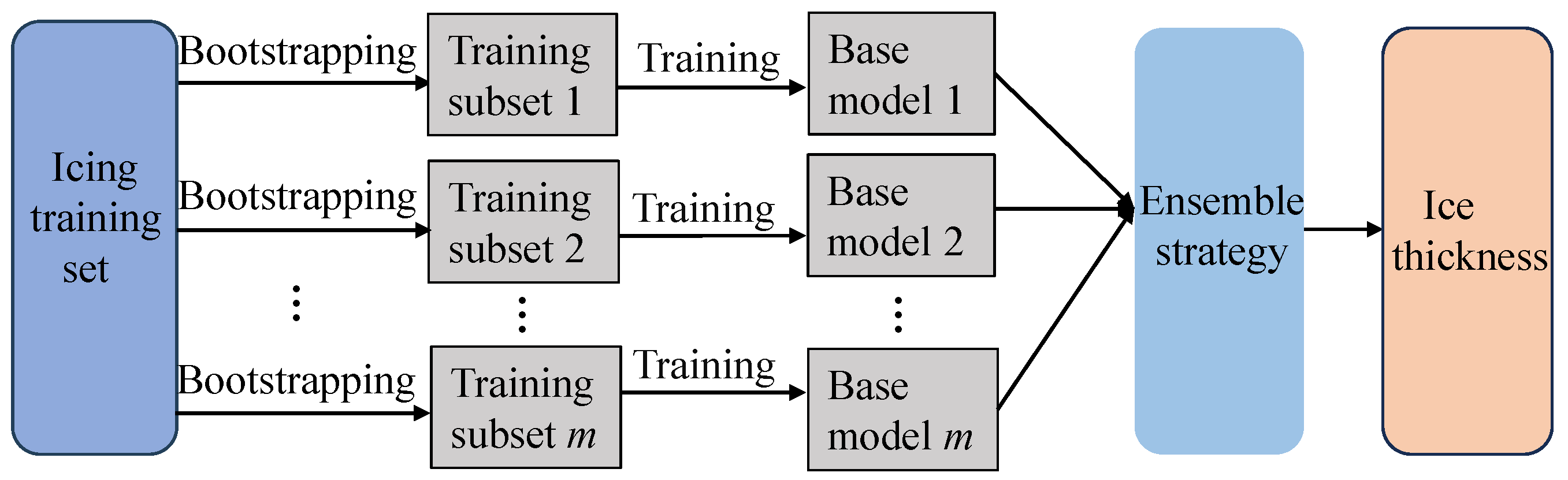
In summary, this chapter has constructed a base model library with diversity in the local area. From the perspective of ensemble model diversity, the base model library introduces sample variation, while different modeling techniques further enhance the diversity of the ensemble. Figure 4 shows a schematic of the base model construction in this section.
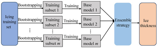
Figure 4.
Illustration of diversity base model generation.
4. Ensemble Strategy of Adaptive Weight
To achieve satisfactory ensemble results, choosing a reasonable prediction fusion strategy is necessary. If the ensemble weights are set to fixed values, it will cause the ensemble model to lose its adaptability, thereby limiting its flexibility and efficacy in practical applications. Therefore, this section designs a two-stage adaptive ice accretion weight allocation strategy to enhance the accuracy of the ice coating prediction model.
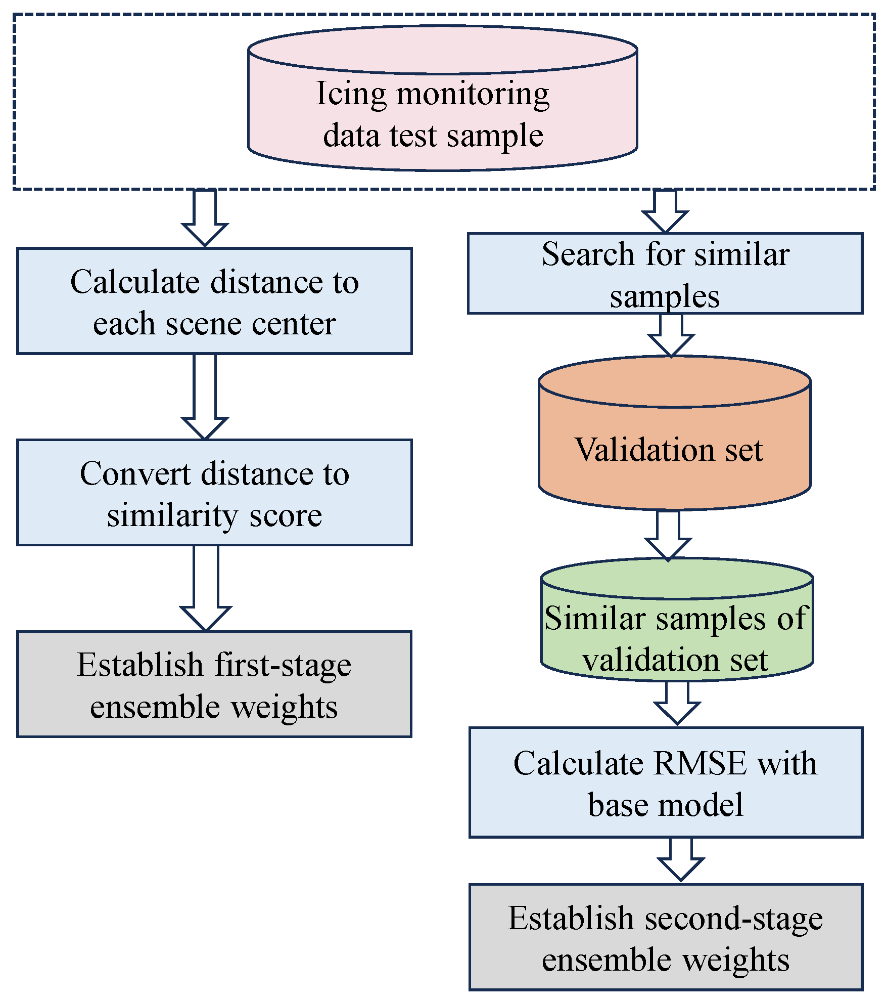
Figure 5 illustrates the design of the two-stage adaptive weights. Firstly, we evaluate the importance of each test set across various scenarios, calculate the first-order weights using Formulas (12) and (13), and obtain the weight of the test data for each local region center. Subsequently, we search for similar small-scale sample sets within each local region, which will be used as inputs to the base model library to obtain the RMSE of each base model. Finally, we calculate and determine the second-order weights according to Formula (15).
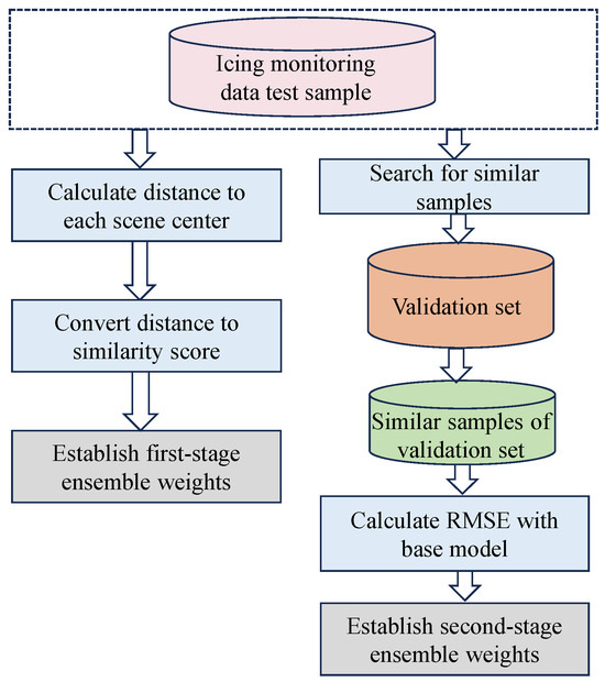
Figure 5.
Schematic diagram of adaptive weighting mechanism.
4.1. Design of First-Stage Adaptive Weights
This paper introduces a scenario weighting mechanism in the initial stage to enhance model performance for each specific scenario. The mechanism evaluates each test dataset’s importance by calculating the similarity to the scenario’s centroid. This similarity measure is then used as a weight, adjusting the contribution of the test dataset to the prediction results for that particular scenario. This approach ensures that predictions are finely tuned to reflect the unique characteristics of each scenario.
The weights are first assigned based on the similarity between the test set data and the scenario dataset in the historical icing monitoring training set. In this section, the Euclidean distance [36] is adopted as the similarity criterion, and the test set is mapped onto the typical scenario centers established in the previous section, and the Euclidean distances between them are computed as described in Equation (12) to assess the similarity between the test data and the historical data of specific microtopography. Ultimately, these similarity values are used to assign weights to each microtopographic weather scenario model:
In order to ensure a total weight of 1, the distance was converted to a similarity score, and the similarity was subsequently normalized to a unit length, with the formulae expressed as follows:
where M represents the number of ice accretion meteorological scenarios, i indicates the index of a local scene, and represents the weight corresponding to the center of the ith ice accretion meteorological scenario in the test data.
4.2. Design of Second-Stage Adaptive Weights
According to the characteristics of the samples and the validation set data of different scenarios, the weights of each base model are dynamically determined. This weight adjustment strategy can more accurately reflect the characteristics of the samples in different scenarios and the adaptive ability of the model, thus improving the accuracy and stability of the prediction model.
For the test sample , in each scenario, the small-scale sample set that is most similar to the predicted sample is found from using the validation set of the scenario, using Euclidean clustering as a similarity metric. is then used as an input for each base model in the scenario to obtain the prediction results, and the root mean square error (RMSE) is subsequently computed for the performance evaluation, thus obtaining the current RMSE of the sample set for each base model:
Subsequently, the model with the smallest RMSE within is selected, signifying the most precise prediction. The MTAES model employs an integration of multiple meteorological scenarios, thus enhancing the predictive performance. It is ensured that denotes the minimum distance from the validation set to the optimal center of the ice accretion meteorological scenario, corresponding to that aligns best with the optimal scenario center. , characterized by a diversity of base models, not only broadens the model’s applicability across various scenarios but also consolidates the robustness of the MTAES model in efficiently managing diverse ice accretion prediction tasks.
In view of this, this study is committed to dynamically and adaptively determining the weights of the ensemble through the prediction performance of the base model on :
where i represents the index of the base model in the local region, and denotes the weight of the test sample set for the ith base model, while m represents the number of scenario-based models.
4.3. Implementation Process
In the prediction stage, this paper employs ensemble learning to enhance the accuracy and stability of the final predictions by integrating the results from various base models. Each base model’s predictions for new samples are weighted based on their performance in the validation set. This weighting facilitates a dynamic, adaptive ensemble that optimally leverages the predictive capabilities of different models. The adaptive weighted prediction process is represented by Algorithm 1. Step 1 involves clustering the training dataset using the M-H-K algorithm to identify scenario centers. Step 2 generates base models for each identified scenario and bootstrap sample. Step 3 computes the first-stage weights for each scenario by measuring the similarity between the test sample and each scenario center. Step 4 then calculates second-stage weights by evaluating the performance of base models on a selected subset of the validation data that is most similar to the test sample. Finally, Step 5 aggregates these weights to produce the final predicted value.
| Algorithm 1 Two-stage adaptive weighting mechanism |
|
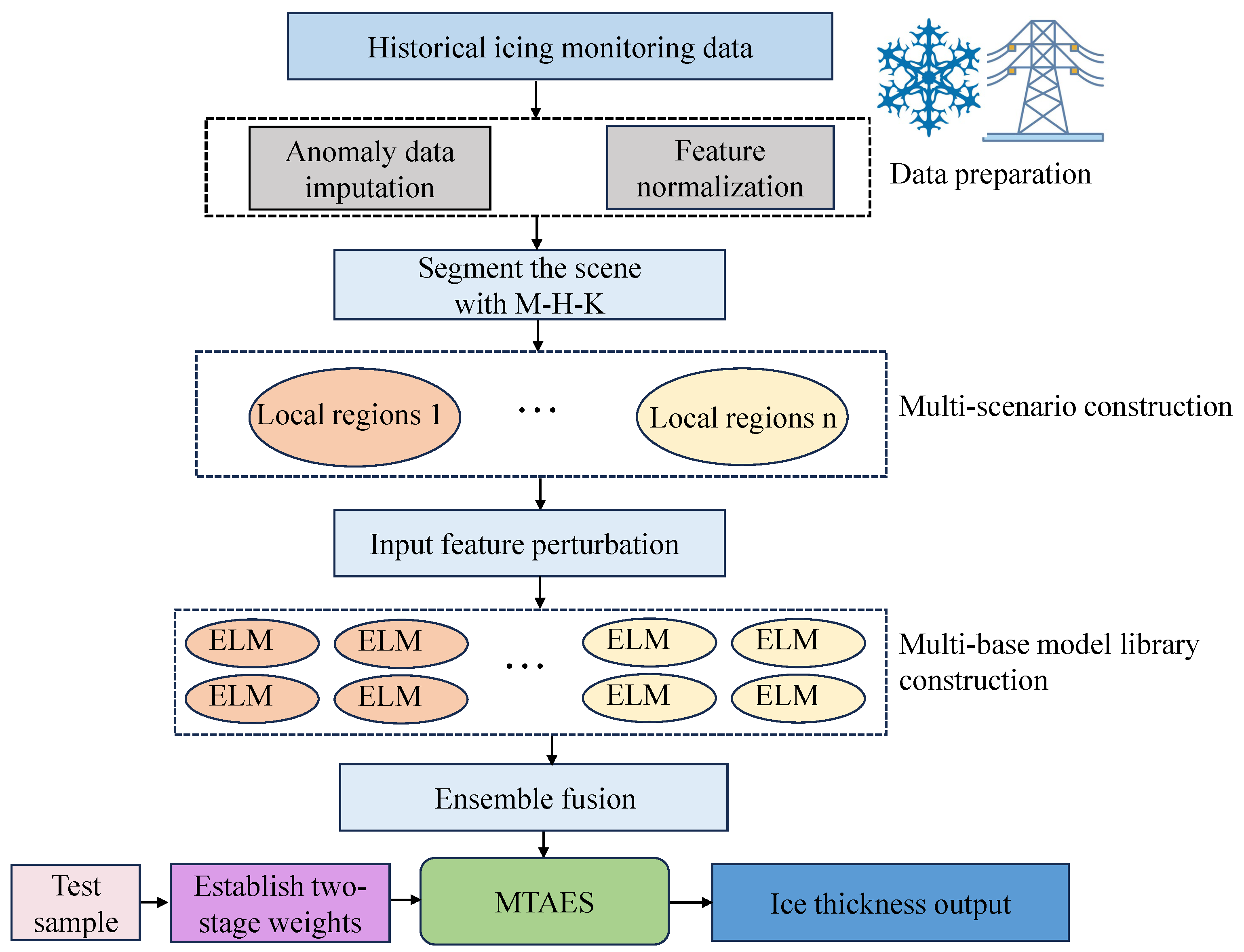
Figure 6 illustrates the prediction-based approach proposed in this study, and the specific implementation process is outlined as follows:
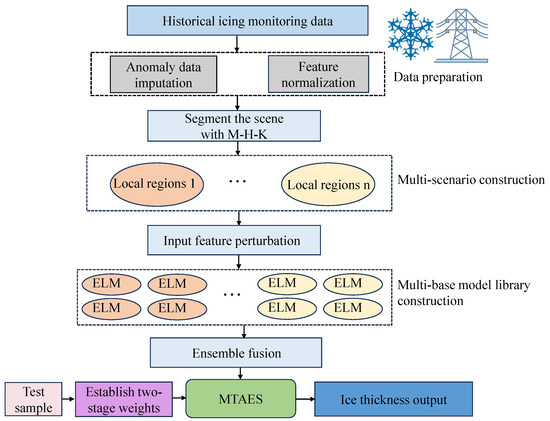
Figure 6.
Ice coating prediction process based on two-stage adaptive weighted ensemble learning.
- Divide the dataset into a training set, testing set, and validation set. Then, cluster the training set using the M-H-K clustering method to divide the data into different typical scenarios and get the clustering center for each scenario.
- Use bootstrap resampling in each scenario to generate multiple different sample subsets. Then, each subset will be trained using ELM to get multiple base models.
- For a new prediction sample x, compute the Euclidean distance between sample x and the clustering center of each scenario as a first-stage weight w.
- For each scenario, find the dataset in the validation set that is most similar to sample x, using the Euclidean distance as a similarity criterion. Input to the models into each subspace to obtain the RMSE evaluation metrics and rank them to determine the weight v of x for each base model in that scenario.
- Based on the first-stage weights w and second-stage weights v obtained from the computation of each prediction sample, the final prediction results are computed by combining the individual outputs of the base model library for that prediction sample.
5. Result and Discussion
To verify the effectiveness of the method proposed in this chapter, this section adopts multiple approaches: initially, preprocessing the data to ensure accuracy and consistency, then evaluating the efficacy of the weight allocation strategy, and, finally, conducting a comparative analysis using several typical prediction models. In this study, the multi-scenario construction process using the M-H-K clustering approach is refined through careful selection and tuning of specific clustering parameters. The initial clustering centers were determined using the Fast-Mean-Shift algorithm, with a bandwidth parameter estimated based on a quantile of 0.2, and a sampling size of 500, ensuring robust initial cluster identification. Subsequently, the Agglomerative Clustering algorithm was applied with no predefined cluster number, using a distance threshold set to 2, to dynamically determine the optimal number of clusters. To ensure the quality of clustering, the DBI was employed to evaluate and select the best K-means configuration. The number of clusters ranged from 2 to the maximum identified by the Agglomerative Clustering, with the final number of clusters and cluster assignments being determined by the configuration yielding the lowest DBI score. This systematic approach to parameter selection enhances the reliability and precision of the clustering results, providing a solid foundation for subsequent prediction models.
5.1. Evaluation Indicators
In this paper, the root mean square error RMSE, regression coefficient , and absolute mean error MAE were used as the evaluation indexes of the experimental results. RMSE is a common statistical index to measure the difference between the predicted value of the prediction model and the measured value of the actual sensor, which helps quantify the error between the predicted result of the model and the measured value of the sensor. When the RMSE value is smaller, the error between the ice thickness predicted by the model and the measured value of the sensor is lower, indicating that the information provided by the model has greater reference significance. MAE is another commonly used evaluation index that measures the average absolute difference between the predicted value of the model and the actual measured value. MAE is calculated by adding the absolute values of all prediction errors and dividing by the number of errors. Unlike RMSE, MAE does not excessively increase the weight due to large error values, providing a more intuitive way to measure model error. The smaller the MAE value, the lower the error between the ice thickness predicted by the model and the actual measured value, and the better the model’s prediction performance. It can intuitively judge the effect of the model. The specific calculation formula for each evaluation is as follows:
where denotes the real ice coating thickness data, is the predicted ice coating thickness data, is the real ice coating thickness mean value, and n is the number of sample points. The smaller the value of RMSE and MAE, the better the model’s performance. The closer the value of is to 1, the better the model fits the data. These metrics can help to more intuitively assess how well the model fits the observations and how accurate the predictions are.
5.2. Data Preparation
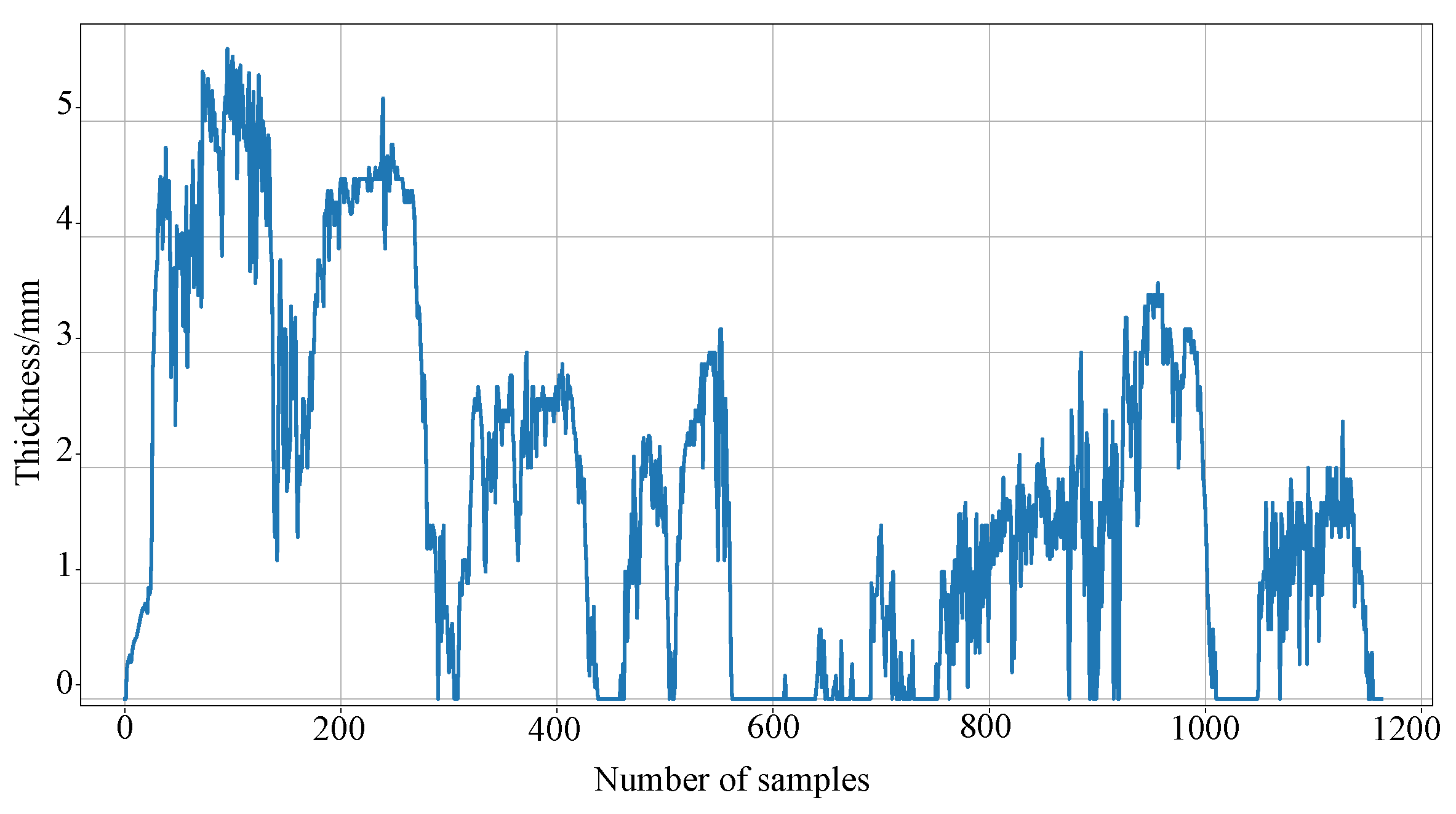
This study used the line ice accretion data collected from a certain city in China from December 2022 to March 2023. To build an effective dataset for training ice accretion prediction models, linear interpolation was applied to rectify outliers and missing values, ensuring the integrity of the dataset. Part of the processed data is displayed as shown in Figure 7. Subsequently, 60% of the samples were selected as the training set, the lower 20% as the validation set, and the remaining 20% as the testing set.

Figure 7.
Visual display of icing data.
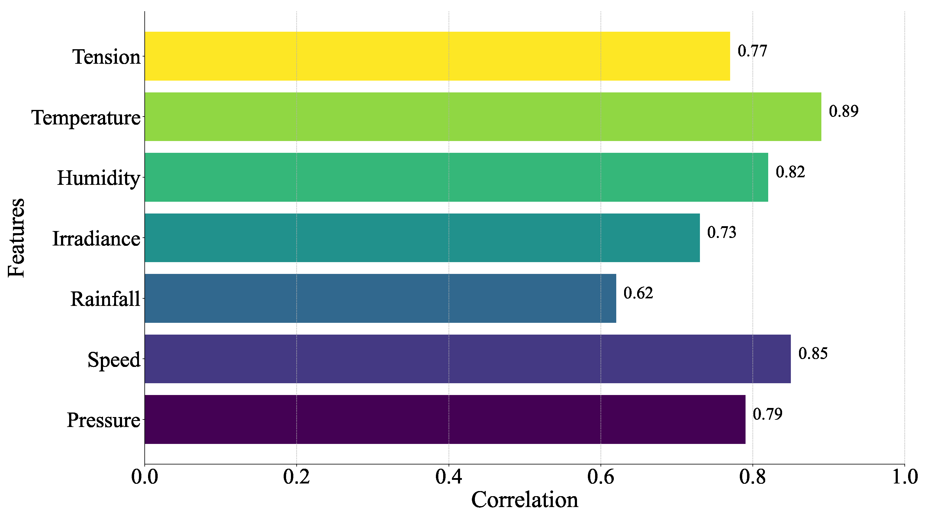
Conductor ice coating is the result of a variety of factors such as micro-meteorology, micro-terrain, conductor characteristics, etc., and, if the input variables are selected according to the actual situation, the prediction model has more influencing factors, which reduces the model efficiency and makes the learning time longer; if the number of inputs is oversimplified, it leads to the reduction of the model prediction accuracy and other problems. Therefore, this paper adopted the gray correlation analysis method to find out the key factors affecting the thickness of wire ice coating, as shown in Figure 8, and it can be found that, relative to other meteorological factors, temperature, wind speed, humidity, and air pressure have a greater influence on the thickness of ice coating. So, we chose these four characteristics as the input of the ice coating prediction model. In addition, we divided the data in this paper into three local areas after PCA according to the optimal DBI index, as shown in Figure 9.
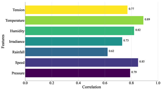
Figure 8.
Feature importance comparison.
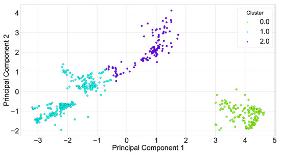
Figure 9.
Scenario clustering visualization.
5.3. Analysis of the Influence of Input Window Length on Model Effect
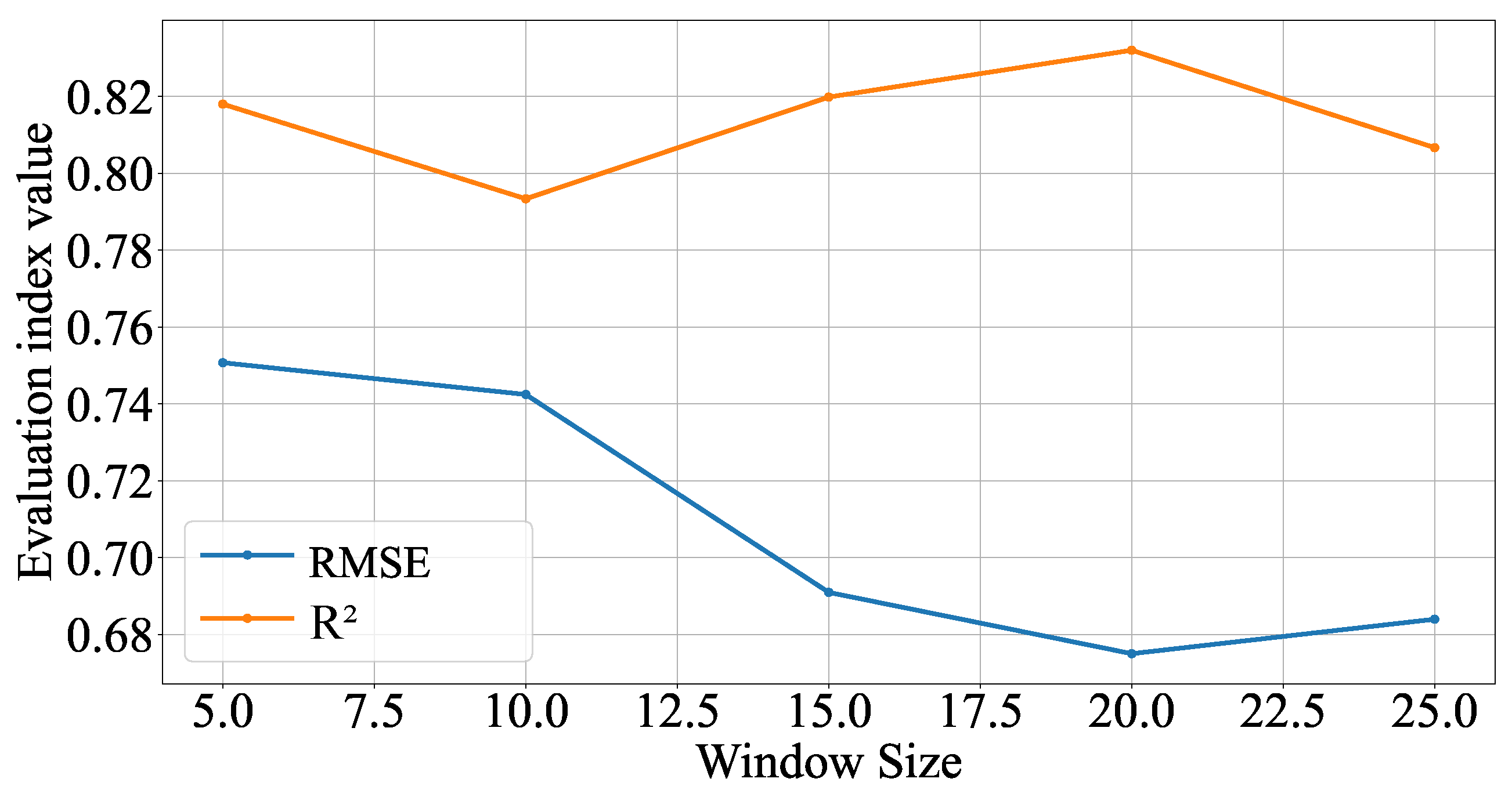
In order to systematically evaluate the impact of sliding window size on the prediction effect of the model, different window sizes were set when using the extreme learning machine process to train the icing dataset in this section to observe the specific impact of window size change on the performance of the model, as shown in Figure 10.
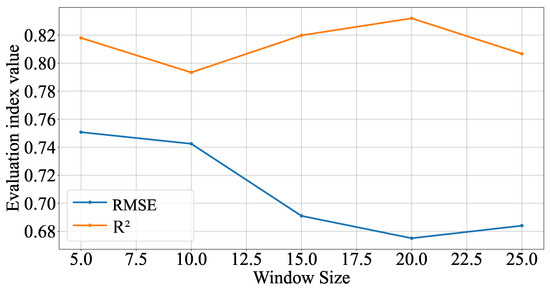
Figure 10.
Effect of sliding window size on prediction performance.
It can be observed from the figure that, with the increase in window size, the root mean square error and determination coefficient of the model show different characteristics. When the window size of RMSE gradually increases from 5 to 10, the prediction performance decreases. However, when the window size continues to increase to 15, RMSE tends to be stable, and then there is a slight upward trend near the window size of 20, indicating that windows that are too large may cause the model to capture unnecessary noise, thus affecting the prediction accuracy. The regression coefficient increases with the increase in window size from the window size of 5, proving that the ability of the model’s explanatory variables continues to improve. The peak value is reached when the window size is 20, indicating that the model’s interpretation ability is the best at this time. After that, as the window size continues to increase to 25, there is a significant decline, and the adaptability of the model to the data characteristics decreases. It can be concluded that the model’s overall performance is ideal when the window size is between 15 and 22. When the window size is 20, the two indicators are optimal. Therefore, this chapter selects 20 as the window size of the prediction model. At this time, the model has a relatively good response speed to historical information and future trends.
5.4. Validation of Weight Allocation Method Effectiveness
The weight allocation mechanism plays a pivotal role in the model, directly influencing the accuracy and reliability of prediction results. Therefore, evaluating the effectiveness of various weight allocation methods is crucial for comprehending and optimizing model performance. The similarity criterion serves as a critical factor in determining weights, with this study primarily employing the Euclidean distance as the measure of similarity. However, for a comprehensive assessment of the model’s adaptability and flexibility, this chapter also investigated the impact of several other distance measurement methods on the predictive performance of the model. The results are presented in Table 1.

Table 1.
The predictive performance of MTAES with different similarity functions.
By comparing the effects of different similarity criteria on model weight allocation and final prediction performance, this paper aims to validate the most suitable distance metric for this model. From Table 1, it can be seen that the Euclidean distance, as the similarity criterion, achieves the best performance, compared with criteria such as the Chebyshev distance, Pearson correlation coefficient (PPMCC), and Euclidean distance with a smaller gap between the performance of the similarity criterion, taking into account that the Euclidean distance has the characteristics of convenient and fast calculation. Considering that the Euclidean distance is convenient and fast to calculate, this paper chose the Euclidean distance as the similarity criterion for two-stage adaptive weighted ensemble prediction.
5.5. Validation of Overall Model Validity
To verify the effectiveness of the methods proposed in this chapter, this study adopted various perspectives and selected several typical prediction models for comparative analysis. SVR represents the global SVR model; the penalty coefficient C was set to 10, and the radial basis function was selected as the kernel function. Pls stands for the global PLS model; the number of components was set to 2, and the zoom data option was selected. Elm represents the global elm model; the activation function was sigmoid, and the hidden layer size was 10. BP represents the global BP model; the activation function was sigmoid, the learning rate was set to 0.1, and the optimizer was Adam. Lstm represents the global LSTM model, with 64 hidden layer neurons and three layers. PSO-SVR refers to the combined model of particle swarm optimization algorithm and support vector machine. The parameters of SVR are optimized by PSO. The particle swarm size was 30, the inertia weight was 0.3, and the learning factor was 0.5. MSEELM- Average represents the elm model based on adaptive selective integration, and the results of the base model are fused in a simple average way. MTAES-k refers to the two-stage integrated prediction of icing multi-regions based on K-means clustering. Its basic idea is to cluster the training sample set directly using k-means to obtain multiple regions, and then generate subsets according to the divided regions to train the base model, and, finally, carry out weighted ensemble prediction. MSOAEELM represents the first-order adaptive weighted integration of regions. The basic idea is to divide regions and allocate weights based on the similarity of the Euclidean distance, and then directly establish a base model in each region without adding the second-stage weighted integration design. The MTAES method, proposed in this chapter, was further compared with models from references [16,19].
The prediction performance of the method proposed in this chapter can be fully assessed by comparing it with the different models mentioned above. In the case study, this chapter will present in detail the prediction results of each model on the same dataset using the evaluation metrics and , and show the comparison results through Table 2 to visualize the advantages and effectiveness of the method proposed in this chapter in ice coating prediction.
Table 2.
The prediction results of different ice thickness prediction methods.
According to the results from Table 2, simply applying traditional global models, such as SVR, PLS, ELM, and BP, does not significantly enhance prediction performance and sometimes even adversely affects the prediction results. When comparing global models that do not utilize ensemble learning strategies with the MTAES model, whether in terms of or , MTAES consistently demonstrates superior performance, emphasizing the importance of using ensemble learning and scenario division.
A further comparison of different ensemble strategies shows that, compared to MSEELM-Average, MTAES displays performance improvements in all cases, proving the effectiveness of incorporating adaptive weight allocation strategies into the model. Particularly, compared to MTAES-K, which is based solely on K-means clustering, the method proposed in this chapter achieves a significant performance improvement after employing a more refined scenario division, with an increase of 0.12 mm in RMSE and a 1.4% improvement in . In order to more intuitively understand the prediction error of each model in each error interval, the number of error samples of each prediction model in each interval is recorded in the form of a table. The prediction error is divided into four intervals: 0–0.5 mm, 0.5–1 mm, 1–2 mm, and more than 2 mm. As shown in Table 3, it can be seen that the prediction error of most samples of the MTAES prediction method is controlled below 0.5 mm, and the number of samples with prediction error greater than 2 mm is 4, which is less than for other models.
Table 3.
The number of samples in the error interval of different icing thickness prediction methods.
In order to visually analyze the predictive effect of the model proposed in this paper, the model prediction curve is plotted for analysis, as shown in Figure 11 for the part of the model used in this chapter to predict the ice coating thickness curve; from the figure, it can be seen that the predicted value of the ice coating thickness of the model proposed in this paper is basically in line with the real value curve; in addition, the model most accurately follows the trend of the actual change of the ice coating thickness, which demonstrates higher accuracy, and proves that the model has better prediction accuracy.
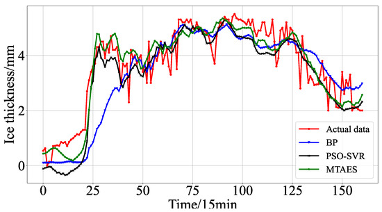
Figure 11.
Comparison between predicted curves of various models and actual values.
Furthermore, to evaluate the applicability of the integrated modeling approach, this paper selected ice sensor data from another line for experimental verification; as depicted in Table 4, the MTAES method proposed in this chapter consistently outperforms other comparative methods in both RMSE and , thereby affirming the efficacy of the model construction approach presented in this paper and the generalizability of the prediction model.
Table 4.
Validation of model design applicability.
5.6. Analysis of the Impact of Prediction Duration on Model Performance
The computational complexity of the proposed model is primarily derived from the training phase of the base model, the extreme learning machine (ELM). Specifically, the complexity is dominated by the operations required to calculate the hidden layer output matrix and the output weights, which can be expressed as , where N is the number of training samples, d is the input dimension, and L is the number of hidden neurons. For the prediction phase, the complexity is , where M is the number of new samples. As the number of hidden neurons or training samples increases, the computational cost grows, particularly due to the term in the training phase.
When predicting the ice coating thickness of transmission lines, the size of the moving step also has an impact on the training effectiveness of the network model. For accurate prediction of future ice coating thickness, there usually is a limitation for too long of a prediction time length. In Table 5, the statistics of the error effects under different prediction lengths are shown. The results show that the present model performs well in the short-term prediction task, but the prediction effect gradually decreases with time. The surface model has high accuracy in the face of short-term prediction but faces challenges in long-term prediction. This may be due to the excessive dynamics of the climate over long time spans leading to the attenuation of the accuracy of the predictions.
Table 5.
The prediction results for different prediction durations.
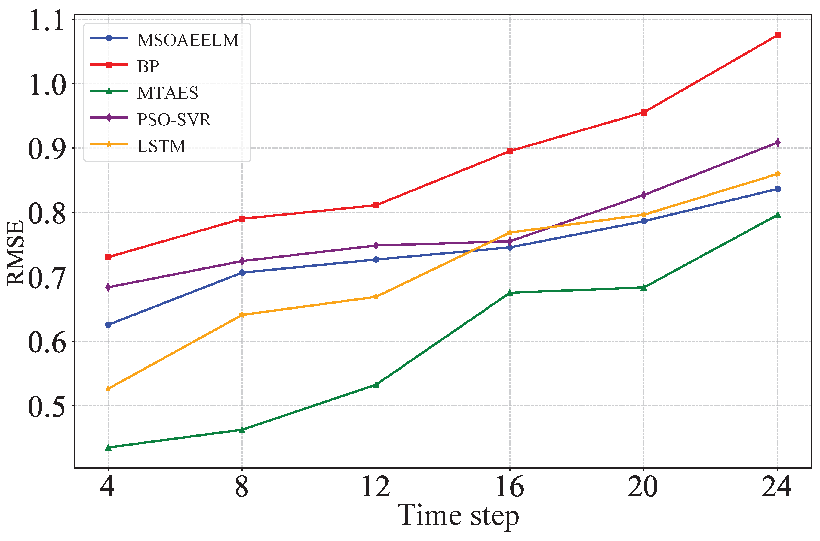
The scalability of the proposed model is a critical consideration, particularly when extending the prediction duration, as it effectively increases the complexity of the time series the model must handle. Therefore, this section also compares the prediction performance of each model as the time step increases, using RMSE as the indicator. As shown in Figure 12, the proposed model consistently outperforms the other models at various time steps, demonstrating its scalability.
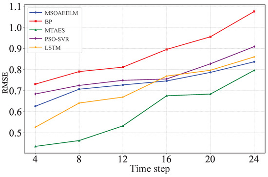
Figure 12.
Comparison of RMSE magnitudes at different time steps.
5.7. Findings and Limitations
The results of our study demonstrate the effectiveness of the M-H-K clustering algorithm in accurately delineating ice coating scenarios, which has significant implications for the field of power grid management. By improving the prediction of ice coating thickness, this method can enhance the reliability and safety of transmission lines during adverse weather conditions. The robustness of the model in handling diverse meteorological scenarios also suggests its potential applicability in other predictive tasks where scenario-based analysis is critical. Moreover, the improved accuracy in prediction can lead to more efficient resource allocation and maintenance scheduling, ultimately reducing operational costs and minimizing downtime.
Despite the promising results, certain limitations of our study should be acknowledged. First, the selection of parameters for the clustering algorithm, while carefully tuned, may not be universally optimal across all datasets or applications. This could potentially limit the generalizability of our findings to other regions or climatic conditions. Second, while the model exhibits robustness in terms of noise tolerance, it has not been extensively tested under extreme outlier scenarios, which may occur during rare but severe weather events. Additionally, the computational complexity associated with the M-H-K clustering method, particularly in large-scale applications, may pose challenges in real-time implementations.
6. Conclusions
Aiming at the problem of the insufficient generalization ability of traditional intelligent icing prediction models under different environmental conditions, a multi-region adaptive ensemble weighting-based icing thickness prediction model is proposed by combining ensemble learning and local modeling ideas. Firstly, a combination clustering method is proposed to improve the division of meteorological regions and perform multi-region division on historical ice cover samples under different meteorological conditions. Subsequently, multiple training subsets were generated using the bagging method in various meteorological regions, and extreme learning machines were used to construct diverse base models. Next, a two-stage adaptive weight allocation mechanism was designed to dynamically allocate output weights for new icing data test samples based on their distance from the regional center and the prediction error of similar samples in the validation set. Subsequently, a two-stage adaptive weighted ensemble ice thickness prediction model, MTAES, was established through adaptive integration using a base model library.
The analysis of experimental results showed that, compared with commonly used prediction models, the MTAES model proposed in this chapter obtained an RMSE of 0.675 and 0.739, of 0.832 and 0.734, and MAE of 0.522 and 0.570, respectively, when tested on two datasets. Compared with commonly used intelligent computing models, it demonstrates better advantages and verifies the effectiveness of local sample region division and adaptive weighting integration in improving the prediction performance of transmission line icing thickness.
Based on the issues encountered during the research, future efforts should include exploring the processing and analysis of ice coating data through enhanced and updated sensors on transmission lines, which will provide more comprehensive data for thorough analysis. Additionally, future research should consider deeper investigations into the mechanisms and influencing factors of ice coating formation to develop a more refined weight allocation mechanism. Incorporating more data sources and features, such as terrain information and line parameters, could further diversify model inputs and improve the overall consideration of the ice coating model. These future research directions will contribute to enhancing the accuracy and reliability of ice coating thickness prediction models, offering more precise support for the safe operation of power systems.
Author Contributions
Conceptualization, Q.C. and H.G.; methodology, H.G. and L.S.; software, H.G. and Q.C.; validation, H.G. and L.S.; formal analysis, H.G.; investigation, H.G. and J.P.; resources, Q.C. and H.G.; data curation, H.G.; writing—original draft preparation, H.G.; writing—review and editing, H.G., Q.C. and L.S.; supervision, Q.C. and S.A.; project administration, H.W. All authors have read and agreed to the published version of the manuscript.
Funding
This research received no external funding.
Data Availability Statement
Dataset available on request from the authors.
Conflicts of Interest
Author Haitao Wu was employed by the State Grid Chongqing Electric Power Company, Electric Power Science Research Institute. The remaining authors declare that the research was conducted in the absence of any commercial or financial relationships that could be construed as a potential conflict of interest.
References
- Hao, Y.; Huang, L.; Wei, J.; Liang, W.; Pan, R.; Yang, L. The Detecting System and Method of Quasi-Distributed Fiber Bragg Grating for Overhead Transmission Line Conductor Ice and Composite Insulator Icing Load. IEEE Trans. Power Deliv. 2023, 38, 1799–1809. [Google Scholar] [CrossRef]
- Bahrami, A.; Yan, M.; Shahidehpour, M.; Pandey, S.; Vukojevic, A.; Paaso, E. Mobile and Portable De-icing Devices for Enhancing the Distribution System Resilience Against Ice Storms Preventive strategies for damage control. IEEE Electrif. Mag. 2021, 9, 120–129. [Google Scholar] [CrossRef]
- Mishra, S.; Tripathy, L. A Critical Fault Detection Analysis & Fault Time in a UPFC Transmission Line. Prot. Control Mod. Power 2019, 4, 1–10. [Google Scholar]
- Xu, X.; Niu, D.; Zhang, L.; Wang, Y.; Wang, K. Ice Cover Prediction of a Power Grid Transmission Line Based on Two-Stage Data Processing and Adaptive Support Vector Machine Optimized by Genetic Tabu Search. Energies 2017, 10, 1862. [Google Scholar] [CrossRef]
- Jones, K.F. Predicting Ice and Snow Loads for Transmission Line Design. Atmos. Res. 1998, 46, 87–97. [Google Scholar] [CrossRef]
- Makkonen, L.; Stallabrass, J. Experiments on the Cloud Droplet Collision Efficiency of Cylinders. J. Appl. Meteorol. Clim. 1987, 26, 1406–1411. [Google Scholar] [CrossRef]
- Lenhard, J. An Indirect Method for Estimating the Weight of Glaze on Wires. Bull. Am. Meteorol. Soc. 1955, 36, 1–5. [Google Scholar] [CrossRef]
- Jiang, X.L.; Han, X.B.; Hu, Y.Y.; Yang, Z.Y. The study of Dynamic Wet-Growth Icing model of insulator. Proc. CSEE 2017, 09, 1–8. [Google Scholar]
- Xu, Q.S.; Lao, J.M.; Hou, W.; Wang, M.L. Real-time Monitoring and Calculation Model of Transmission Lines Nequal Ice-Coating. High Volt. Technol. 2009, 35, 2865–2869. [Google Scholar]
- Vaziri, P.; Ahmadi, S.; Daneshfar, F.; Sedaee, B.; Alimohammadi, H.; Rasaei, M.R. Machine Learning Techniques in Enhanced Oil Recovery Screening Using Semisupervised Label Propagation. SPE J. 2024, 1–22. [Google Scholar] [CrossRef]
- Othmani, A.; Brahem, B.; Haddou, Y. Machine-Learning-Based Approaches for Post-Traumatic Stress Disorder Diagnosis Using Video and EEG Sensors: A Review. IEEE Sens. J. 2023, 23, 24135–24151. [Google Scholar] [CrossRef]
- Zheng, Z.H.; Liu, J.S. Prediction Method of Ice Thickness on Transmission Lines Based on the Combination of GA and BP Neural Network. Power Syst. Clean Energy 2014, 30, 27–30. [Google Scholar]
- Liu, J.; Li, A.J.; Zhao, L.P. Prediction Model Based on Fuzzy and T-S Neural Network for Ice Thickness. Hunan Electr. Power 2012, 32, 1–4. [Google Scholar]
- Yin, Z.R.; Su, X.L. Icing Thickness Forecasting of Transmission Line Based on Particle Swarm Algorithm to Optimize SVM. J. Electr. Power 2014, 29, 6–9. [Google Scholar]
- Sun, W.; Wang, C. Staged Icing Forecasting of Power Transmission Lines Based on Icing Cycle and Improved Extreme Learning Machine. J. Clean. Prod. 2019, 208, 1384–1392. [Google Scholar] [CrossRef]
- Dai, D.; Huang, X.T. Prediction of Transmission Line Icing Based on Support Vector Machine Model. High Volt. Technol. 2013, 39, 2822–2828. [Google Scholar]
- Huang, X.B.; Wang, Y.X.; Zhu, Y.C. Icing Forecast of Transmission Line Based on Genetic Algorithm and Fuzzy Logic. High Volt. Technol. 2016, 42, 1228–1235. [Google Scholar]
- Xiong, W.; Xu, H.; Xu, L.X.; Zhu, K.F.; Yi, B.S. Combined Model of Icing Prediction of Transmission Lines Based on RF-APJA-MKRVM Considering Time Cumulative Effect. High Volt. Technol. 2022, 48, 948–957. [Google Scholar]
- Xu, X.; Niu, D.; Wang, P. The Weighted Support Vector Machine Based on Hybrid Swarm Intelligence Optimization for Icing Prediction of Transmission Line. Math. Probl. Eng. 2015, 4, 1–9. [Google Scholar] [CrossRef]
- Xiong, W.; Yuan, H.J.; You, L. Prediction Method of Icing Thickness of Transmission Line Based on MEAO. Clust. Comput. 2018, 21, 845–853. [Google Scholar] [CrossRef]
- Chen, Y.; Li, P.; Zhang, Z.J. Online Prediction Model for Power Transmission Line Icing Load Based on PCA-GA-LSSVM. Power Syst. Prot. Control 2019, 47, 110–119. [Google Scholar]
- Ma, T.N.; Niu, D.X.; Fu, M. Icing Forecasting for Power Transmission Lines Based on a Wavelet Support Vector Machine Optimized by a Quantum Fireworks Algorithm. Appl. Sci. 2016, 6, 54. [Google Scholar] [CrossRef]
- Zhu, Y.S.; Huang, X.B.; Jia, J.Y. Numerical Simulation for icing and Influence on Transmission Line. J. Xi’an Jiaotong 2015, 49, 120–125. [Google Scholar]
- Zhou, R.; Zhang, Z.; Yan, Z. GPR-based High-precision Passive-support Fiber Ice Coating Detection Method for Power Transmission Lines. Opt. Express 2021, 29, 30483–30493. [Google Scholar] [CrossRef] [PubMed]
- Mahesh, B. Machine learning Algorithms—A Review. Int. J. Sci. Res. 2020, 9, 381–386. [Google Scholar] [CrossRef]
- Wen, Y.F.; Cui, L.J.; Sun, Y. Non-intrusive load decomposition method considering state probability factors and state corrections. Power Syst. Tech. 2019, 43, 4178–4184. [Google Scholar]
- Heredia, C.; Moreno, S.; Yushimito, W.F. Characterization of Mobility Patterns with a Hierarchical Clustering of Origin-Destination GPS Taxi Data. IEEE Trans. Intell. Transp. Syst. 2022, 23, 12700–12710. [Google Scholar] [CrossRef]
- Davies, D.L.; Bouldin, D.W. A Cluster Separation Measure. IEEE Trans. Pattern Anal. 1979, 2, 224–227. [Google Scholar] [CrossRef]
- Jiang, F.; Lin, Z.Y.; Wang, W.Y. Optimal Bagging Ensemble Ultra Short Term Multi-energy Load Forecasting Considering Least Average Envelope Entropy Load Decomposition. Proc. CSEE 2024, 44, 1777–1789. [Google Scholar]
- Wang, X.; Hu, T.; Tang, L. A multiobjective Evolutionary Nonlinear Ensemble Learning with Evolutionary Feature Selection for Silicon Prediction in Blast Furnace. IEEE Trans. Neural Netw. Learn. Syst. 2022, 33, 2080–2093. [Google Scholar] [CrossRef]
- You, W.X.; Shen, K.; Yang, N. Electricity Theft Detection Based on Bagging Heterogeneous Ensemble Learning. Autom. Electr. Power Syst. 2021, 45, 105–113. [Google Scholar]
- Huang, G.B.; Zhu, Q.Y.; Siew, C.K. Extreme Learning Machine: Theory and Applications. Neurocomputing 2006, 70, 489–501. [Google Scholar] [CrossRef]
- Xiao, C.; Sutanto, D.; Muttaqi, K.M.; Zhang, M.; Meng, K.; Dong, Z.Y. Online Sequential Extreme Learning Machine Algorithm for Better Predispatch Electricity Price Forecasting Grids. IEEE Trans. Ind. Appl. 2021, 57, 1860–1871. [Google Scholar] [CrossRef]
- Shi, X.; Kang, Q.; An, J.; Zhou, M. Novel L1 Regularized Extreme Learning Machine for Soft-Sensing of an Industrial Process. IEEE Trans. Ind. Inform. 2022, 18, 1009–1017. [Google Scholar] [CrossRef]
- Ye, L.; Ma, M.S.; Jing, J.X.; Li, Z.; Li, J.C.; Zhou, T.P. Factor Analysis-extreme Learning Machine Aggregation Method Considering Correlation of Wind Power and Photovoltaic Power. Autom. Electr. Power Syst. 2021, 45, 31–40. [Google Scholar]
- Jiang, J.; Wen, Z.; Zhao, M. Series arc Detection and Complex Load Recognition Based on Principal Component Analysis and Support Vector Machine. IEEE Access 2019, 7, 47221–47229. [Google Scholar] [CrossRef]


Disclaimer/Publisher’s Note: The statements, opinions and data contained in all publications are solely those of the individual author(s) and contributor(s) and not of MDPI and/or the editor(s). MDPI and/or the editor(s) disclaim responsibility for any injury to people or property resulting from any ideas, methods, instructions or products referred to in the content. |
© 2024 by the authors. Licensee MDPI, Basel, Switzerland. This article is an open access article distributed under the terms and conditions of the Creative Commons Attribution (CC BY) license (https://creativecommons.org/licenses/by/4.0/).