A Full-Stage Productivity Equation for Constant-Volume Gas Reservoirs and Its Application

Abstract

Gas well production involves various stages, including stable, variable, and declining production. However, existing production-capacity equations typically apply only to the stable production stage, limiting their effectiveness in evaluating gas well productivity across all stages. To address this, the material balance equation and Darcy’s equation were employed to account for changes in average formation pressure due to pressure drop funnels. The concept of a pressure-conversion skin factor was introduced, and its approximation was developed, leading to the establishment and solution of a full-stage productivity equation. Numerical simulations were then conducted to verify the accuracy and applicability of this equation. The findings are as follows: ① The full-stage productivity equation remains effective even when production rates and pressure are not constant, with the only potential source of inaccuracy being the approximative solution for the pressure conversion-skin factor. ② Numerical simulations demonstrated that the approximate solution closely matched the numerical simulation results for average formation pressure across various production stages and fundamental parameters, showing a consistent trend and high precision. The approximate and independent approximation solutions for absolute open-flow capacity were nearly identical, indicating the full-stage productivity equation’s applicability throughout the production of gas wells. ③ Application results revealed that the full-stage productivity equation offers superior accuracy compared to the modified isochronous well test. ④ The approximate solution generally provides slightly higher accuracy, and the independent approximate solution effectively eliminates the influence of gas leakage radius. Therefore, the use of the approximate solution is recommended to calculate the average formation pressure and the independent approximate solution to calculate the absolute open-flow capacity. The full-stage productivity equation developed in this study is not constrained by the production system, making it suitable for productivity evaluation across all stages of gas well production. This has significant implications for the effective development of gas fields.

1. Introduction

Production-capacity equations describe the relationships among gas output, formation pressure, and bottomhole flow pressure in gas wells, forming a fundamental theory in gas field development [1,2,3]. Typically, gas well production is represented on the right side of the productivity equation, while formation pressure and bottomhole flow pressure are placed on the left side. Depending on how production is expressed on the right side, these equations can take various forms, such as monomial, binomial, trinomial, one-point, and exponential equations. Li et al. and Yang et al. developed a monomial capacity equation based on Darcy’s law of seepage [4,5]. Building on this, the binomial capacity equation was established by incorporating the effects of non-Darcy seepage [4,5]. Further extending the binomial equation, Cheng et al. and Xiao et al. accounted for the starting pressure gradient, leading to the development of a trinomial capacity equation [6,7]. Meanwhile, Al-Attar et al. and Chen et al. simplified the binomial equation to create a one-point capacity equation [8,9]. Kalantariasl et al. and Liang et al. introduced an exponential capacity equation, essentially an empirical model derived from fitting production data [10,11]. The monomial, binomial, and trinomial equations can be further categorized based on the pressure form on the left side of the equation—pseudo pressure, pressure squared, or pressure. Among these, the pseudo-pressure form is the most rigorously derived mathematically. Zhuang et al., Sun et al., Tan et al., and Tian et al. simplified the pseudo pressure, developing the pressure-squared and pressure forms of production-capacity equations [12,13,14,15]. Additionally, research by Li et al. indicates that the one-point method and exponential forms generally exist only in the pressure form [16,17].

The physical model and production system determine the applicability of various production-capacity equations, with the former establishing the scope of application and the latter defining the specific application stage. Since there are connections between different forms of capacity equations, the binomial, trinomial, one-point, and exponential capacity equations can all be seen as simplified versions of the monomial capacity equation. Similarly, the pressure-squared and pressure forms of capacity equations can be viewed as simplified versions of the pseudo-pressure form. As such, the monomial capacity equation is the foundation for studying the conditions under which different capacity equations apply.

Physical models are typically created using the monomial productivity equation, assuming constant-volume gas reservoirs. These models account for factors such as non-Darcy flow [18,19], skin factor [20,21,22], stress sensitivity [23,24], slippage effect [25,26], start-up pressure gradient [27,28,29], retrograde condensation [30,31,32], gas–water two-phase flow [33,34], and fractures [35,36,37]. By adjusting these parameters domestically and internationally, scholars have developed capacity equations tailored to various physical models. For instance, Ehibor et al., Liu et al., and Ogunrewo et al. considered the two-phase gas flow and condensate oil to establish the capacity equation for condensate gas reservoirs [38,39,40]. Wang et al. developed the capacity equation for abnormally high-pressure gas reservoirs by considering stress sensitivity [41,42], while Du et al. and Hu et al. integrated factors such as stress sensitivity, non-Darcy seepage, and fractures to establish the capacity equation for carbonate gas reservoirs [43,44]. Li et al. and Wei et al. focused on gas–water two-phase flow and the start-up pressure gradient to develop the capacity equation for water-producing gas reservoirs [45,46,47]. By accounting for different influencing factors, the application scope of these capacity equations has been expanded.

When constructing a monomial production-capacity equation, the production system is typically assumed to operate at a fixed rate by Li et al. and Yang et al., which is suitable for the stable production phase [4,5]. However, this assumption limits the validity of these equations to the stable production phase, as they do not account for changes in the production system. Gas well production generally undergoes several stages, including stable production, variable production, and decline. Although researchers like Zeng et al., Li et al., and Gao et al. have studied stable production technology, gas production rules, and development effects for various types of gas reservoirs [48,49,50], the lack of capacity equations for the variable and decline stages has hindered the evaluation of gas well productivity across different stages. Therefore, there is an urgent need to establish a full-stage production-capacity equation that can unify all production stages.

The authors used the material balance and Darcy equations to improve a productivity equation’s applicability while accounting for the average formation pressure change using the pressure drop funnel. The pressure-conversion skin is presented, a full-stage productivity equation is formulated and solved for the first time, and a numerical simulation is used to verify the solution’s applicability. The research of this paper represents the first time the applicable stage of the production-capacity equation is expanded to the full-stage of gas well production, including the different stages of fixed production, variable production, and decreasing production, and the numerical model validation and example application show high accuracy, which is of great significance for realizing the effective development of the gas field.

2. Mathematical Model

2.1. Darcy Equation

A circular, homogenous, horizontal, fixed-volume gas reservoir with similar thickness is centered around the gas well. Darcy’s law-based differential equation for radial gas plane seepage at any time t under the standard state and common unit system on the ground is

$$q_{\mathrm{sc}}\left(r,t\right)={\displaystyle \frac{Z_{\mathrm{sc}}{T}_{\mathrm{sc}}}{p_{\mathrm{sc}}}}{\displaystyle \frac{p\left(r,t\right)}{Z\left(p\right)T}}{\displaystyle \frac{\mathrm{86,400}}{{10}^6}}{\displaystyle \frac{2\pi rhK}{\mu \left(p\right)}}{\displaystyle \frac{\mathrm{d}p\left(r,t\right)}{\mathrm{d}r}}$$

(1)

where q_sc(r,t) is the gas volume flow rate at radius r at t in the ground standard state, m³/d; Z_sc is the standard deviation coefficient, dimensionless; T_sc is the standard temperature, K; p(r,t) is the formation pressure at radius r at t, MPa; p_sc is the standard pressure, MPa; Z(p) is the deviation coefficient corresponding to p(r,t), dimensionless; T is the reservoir temperature, K; 86,400/10⁶ is the conversion coefficient from Darcy units to standard units, dimensionless; K is the reservoir permeability, 10⁻³ μm²; μ(p) is the gas viscosity corresponding to p(r,t), mPa·s; r is any radius from the center of the reservoir, m; and h is the reservoir thickness, m.

The solution of r as the unique variable at a fixed time t, where t equals a constant, is the foundation for deriving Equations (2)–(4). Throughout the derivation process, q_sc(r,t) and p(r,t) remain constant with t. From Equation (1), the variables are removed and integrated to obtain

$${\displaystyle {\int }_{r_{\mathrm{w}}}^{r_{\mathrm{e}}}\frac{q_{\mathrm{sc}}\left(r,t\right)}{r}\mathrm{d}r}={\displaystyle \frac{\mathrm{86,400}}{{10}^6}}{\displaystyle \frac{\pi Z_{\mathrm{sc}}{T}_{\mathrm{sc}}}{p_{\mathrm{sc}}}}{\displaystyle \frac{Kh}{T}}{\displaystyle {\int }_{p_{\mathrm{wf}}\left(t\right)}^{p_{\mathrm{e}}\left(t\right)}\frac{2p\left(r,t\right)}{\mu \left(p\right)Z\left(p\right)}\mathrm{d}p\left(r,t\right)}$$

(2)

where r_w is the wellbore radius, m; r_e is the gas-release radius, m; p_wf(t) is the bottomhole flow pressure, MPa; and p_e(t) is the boundary pressure, MPa.

The following is the definition of pseudo pressure:

$$\psi \left(p\right)={\displaystyle {\int }_{p_0}^p\frac{2p\left(r,t\right)}{\mu \left(p\right)Z\left(p\right)}\mathrm{d}p\left(r,t\right)}$$

(3)

where ψ(p) is the pseudo pressure corresponding to the pressure p, MPa²/mPa·s; p is the pressure, MPa; and p₀ is the reference pressure, MPa.

Equation (2) should be substituted with Equation (3) to obtain the goal equation.

The target equation is derived by substituting Equation (3) into the integral term at the right end of Equation (2):

$$\psi \left(p_{\mathrm{e}}\right)-\psi \left(p_{\mathrm{wf}}\right)={\displaystyle \frac{{10}^6}{\mathrm{86,400}}}{\displaystyle \frac{p_{\mathrm{sc}}}{\pi Z_{\mathrm{sc}}{T}_{\mathrm{sc}}}}{\displaystyle \frac{T}{Kh}}{\displaystyle {\int }_{r_{\mathrm{w}}}^{r_{\mathrm{e}}}\frac{q_{\mathrm{sc}}\left(r,t\right)}{r}\mathrm{d}r}$$

(4)

where ψ(p_e) is the pseudo pressure corresponding to the boundary pressure p_e(t), and MPa²/mPa s; ψ(p_wf) is the pseudo pressure corresponding to the bottomhole flow pressure p_wf(t), MPa²/mPa s.

The gas well productivity equation for stable flow can be established by substituting q_sc(r,t) = q_sc(t) into Equation (4) when the gas is in a steady flow. In an unstable flow, q_sc(r,t) varies as a function of r and t. Equation (4) can establish the gas well productivity equation under unstable flow by obtaining and substituting the expression for q_sc(r,t).

2.2. Material Balance Equation

Circular fixed-volume gas reservoirs are created by gas wells using just elastic expansion. For any radius r to r_e reservoir, the material balance equation is

$${\displaystyle \frac{{\overline{p}}_{\mathrm{r}}\left(r,t\right)}{Z_{\mathrm{r}}\left(r,t\right)}}={\displaystyle \frac{p_{\mathrm{i}}}{Z_{\mathrm{i}}}}{\displaystyle \frac{G\left(r\right)-G_{\mathrm{p}}\left(r,t\right)}{G\left(r\right)}}$$

(5)

where ${\overline{p}}_r\left(r,t\right)$ is the average formation pressure of the reservoir from r to r_e at time t, MPa; Z_r(r,t) is the corresponding deviation coefficient, dimensionless; p_i is the original formation pressure, MPa; Z_i is the deviation coefficient corresponding to p_i, dimensionless; G(r) is the original geological reserve of the reservoir from r to r_e, m³; and G_p(r,t) is the cumulative wellhead gas production of the reservoir from r to r_e at time t, m³.

For G(r), the expression is

$$G\left(r\right)=\pi \left({r_{\mathrm{e}}}^2-r^2\right)h\varphi S_{\mathrm{gi}}{\displaystyle \frac{Z_{\mathrm{sc}}{T}_{\mathrm{sc}}}{p_{\mathrm{sc}}T}}{\displaystyle \frac{p_{\mathrm{i}}}{Z_{\mathrm{i}}}}$$

(6)

where ɸ represents the porosity of the reservoir, dimensionless; and S_gi is the original gas saturation of the reservoir, dimensionless.

The left and right ends of Equation (5) are derived for t, and then Equation (6) is substituted into Equation (5); this results in

$$q_{\mathrm{sc}}\left(r,t\right)=-\pi \left({r_{\mathrm{e}}}^2-r^2\right)h\varphi S_{\mathrm{gi}}{\displaystyle \frac{Z_{\mathrm{sc}}{T}_{\mathrm{sc}}}{p_{\mathrm{sc}}T}}{\displaystyle \frac{\partial }{\partial t}}\left({\displaystyle \frac{{\overline{p}}_{\mathrm{r}}\left(r,t\right)}{Z_{\mathrm{r}}\left(r,t\right)}}\right)$$

(7)

When r = r_w, ${\overline{p}}_{\mathrm{r}}\left(r_{\mathrm{w}},t\right)$ = ${\overline{p}}_{\mathrm{r}}\left(t\right)$, Equation (7) becomes

$$q_{\mathrm{sc}}\left(t\right)=-\pi \left({r_{\mathrm{e}}}^2-{r_{\mathrm{w}}}^2\right)h\varphi S_{\mathrm{gi}}{\displaystyle \frac{Z_{\mathrm{sc}}{T}_{\mathrm{sc}}}{p_{\mathrm{sc}}T}}{\displaystyle \frac{\mathrm{d}}{\mathrm{d}t}}\left({\displaystyle \frac{{\overline{p}}_{\mathrm{r}}\left(t\right)}{Z_{\mathrm{r}}\left(t\right)}}\right)$$

(8)

where q_sc(t) is the wellhead gas production at time t, m³/d; ${\overline{p}}_{\mathrm{r}}\left(t\right)$ is the average formation pressure from r_w to r_e reservoir at time t, MPa; and Z_r(t) is the deviation coefficient corresponding to ${\overline{p}}_{\mathrm{r}}\left(t\right)$, dimensionless.

Equations (7) and (8) are derived by dividing the left and right ends, respectively:

$${\displaystyle \frac{q_{\mathrm{sc}}\left(r,t\right)}{q_{\mathrm{sc}}\left(t\right)}}={\displaystyle \frac{{r_{\mathrm{e}}}^2-r^2}{{r_{\mathrm{e}}}^2-{r_{\mathrm{w}}}^2}}{\displaystyle \frac{\frac{\partial }{\partial t}\left(\frac{{\overline{p}}_{\mathrm{r}}\left(r,t\right)}{Z_{\mathrm{r}}\left(r,t\right)}\right)}{\frac{\mathrm{d}}{\mathrm{d}t}\left(\frac{{\overline{p}}_{\mathrm{r}}\left(t\right)}{Z_{\mathrm{r}}\left(t\right)}\right)}}$$

(9)

Either the volumetric approach or the isothermal compression factor will ultimately lead to the derivation of Equation (9), for which it can be demonstrated that Equation (9) is accurate. Equation (9) includes ${\overline{p}}_{\mathrm{r}}\left(r,t\right)$ and ${\overline{p}}_{\mathrm{r}}\left(t\right)$. The expressions are, respectively,

$${\overline{p}}_{\mathrm{r}}\left(r,t\right)={\displaystyle \frac{{\displaystyle {\int }_r^{r_{\mathrm{e}}}p\left(r,t\right)\mathrm{d}V}}{{\displaystyle {\int }_r^{r_{\mathrm{e}}}\mathrm{d}V}}}={\displaystyle \frac{2{\displaystyle {\int }_r^{r_{\mathrm{e}}}p\left(r,t\right)r\mathrm{d}r}}{{r_{\mathrm{e}}}^2-r^2}}$$

(10)

$${\overline{p}}_{\mathrm{r}}\left(t\right)={\displaystyle \frac{{\displaystyle {\int }_{r_{\mathrm{w}}}^{r_{\mathrm{e}}}p\left(r,t\right)\mathrm{d}V}}{{\displaystyle {\int }_{r_{\mathrm{w}}}^{r_{\mathrm{e}}}\mathrm{d}V}}}={\displaystyle \frac{2{\displaystyle {\int }_{r_{\mathrm{w}}}^{r_{\mathrm{e}}}p\left(r,t\right)r\mathrm{d}r}}{{r_{\mathrm{e}}}^2-{r_{\mathrm{w}}}^2}}$$

(11)

where dV is the differential of gas volume, dV = 2πrhφS_gdr, m³.

It can be observed from Equations (10) and (11) that ${\overline{p}}_{\mathrm{r}}\left(r,t\right)$, ${\overline{p}}_{\mathrm{r}}\left(t\right)$ represent the volume weighted average of p(r,t). P(r,t) increases with r because it obeys the Darcy flow; this changing p(r,t) curve with r is known as a pressure drop funnel. As r increases, ${\overline{p}}_{\mathrm{r}}\left(r,t\right)$ also shows a gradually outward increasing pressure drop funnel shape. When r = r_w, ${\overline{p}}_{\mathrm{r}}\left(r,t\right)$ is ${\overline{p}}_{\mathrm{r}}\left(t\right)$, and ${\overline{p}}_{\mathrm{r}}\left(t\right)$ are the minimum values of ${\overline{p}}_{\mathrm{r}}\left(r,t\right)$. ${\overline{p}}_{\mathrm{r}}\left(r,t\right)$ and ${\overline{p}}_{\mathrm{r}}\left(t\right)$ are always equal if it is believed that p(r,t) does not change with r, and ignoring the possibility of a pressure drop funnel. It is possible to reduce the derivative term in Equation (9). However, derivation should be considered, as reality does not support this assumption.

2.3. Full-Stage Productivity Equation

Replace Equation (9) with Equation (4) and use derivation to arrive at the following conclusion:

$$\psi \left(p_{\mathrm{e}}\right)-\psi \left(p_{\mathrm{wf}}\right)={\displaystyle \frac{{10}^6}{\mathrm{86,400}}}{\displaystyle \frac{p_{\mathrm{sc}}}{\pi Z_{\mathrm{sc}}{T}_{\mathrm{sc}}}}{\displaystyle \frac{T{q}_{\mathrm{sc}}\left(t\right)}{Kh}}{\displaystyle {\int }_{r_{\mathrm{w}}}^{r_{\mathrm{e}}}\frac{1}{{r_{\mathrm{e}}}^2-{r_{\mathrm{w}}}^2}\frac{{r_{\mathrm{e}}}^2-r^2}{r}\frac{\frac{\partial }{\partial t}\left(\frac{{\overline{p}}_{\mathrm{r}}\left(r,t\right)}{Z_{\mathrm{r}}\left(r,t\right)}\right)}{\frac{\mathrm{d}}{\mathrm{d}t}\left(\frac{{\overline{p}}_{\mathrm{r}}\left(t\right)}{Z_{\mathrm{r}}\left(t\right)}\right)}\partial r}$$

(12)

Starting from Equation (3), and based on the additivity of the integration interval, the following exists between the pseudo pressures:

$${\displaystyle {\int }_{p_{\mathrm{wf}}\left(t\right)}^{p_{\mathrm{e}}\left(t\right)}\frac{2p\left(r,t\right)}{\mu \left(p\right)Z\left(p\right)}\mathrm{d}p\left(r,t\right)}={\displaystyle {\int }_{p_{\mathrm{wf}}\left(t\right)}^{{\overline{p}}_{\mathrm{r}}\left(t\right)}\frac{2p\left(r,t\right)}{\mu \left(p\right)Z\left(p\right)}\mathrm{d}p\left(r,t\right)}-{\displaystyle {\int }_{p_{\mathrm{e}}\left(t\right)}^{{\overline{p}}_{\mathrm{r}}\left(t\right)}\frac{2p\left(r,t\right)}{\mu \left(p\right)Z\left(p\right)}\mathrm{d}p\left(r,t\right)}$$

(13)

Substitute Equation (13) into Equation (12) and derive

$$\psi \left({\overline{p}}_{\mathrm{r}}\right)-\psi \left(p_{\mathrm{wf}}\right)={\displaystyle \frac{{10}^6}{\mathrm{86,400}}}{\displaystyle \frac{p_{\mathrm{sc}}}{\pi Z_{\mathrm{sc}}{T}_{\mathrm{sc}}}}{\displaystyle \frac{T{q}_{\mathrm{sc}}\left(t\right)}{Kh}}{\displaystyle {\int }_{r_{\mathrm{w}}}^{r_{\mathrm{e}}}\frac{1}{{r_{\mathrm{e}}}^2-{r_{\mathrm{w}}}^2}\frac{{r_{\mathrm{e}}}^2-r^2}{r}\frac{\frac{\partial }{\partial t}\left(\frac{{\overline{p}}_{\mathrm{r}}\left(r,t\right)}{Z_{\mathrm{r}}\left(r,t\right)}\right)}{\frac{\mathrm{d}}{\mathrm{d}t}\left(\frac{{\overline{p}}_{\mathrm{r}}\left(t\right)}{Z_{\mathrm{r}}\left(t\right)}\right)}\partial r}+{\displaystyle {\int }_{p_{\mathrm{e}}\left(t\right)}^{{\overline{p}}_{\mathrm{r}}\left(t\right)}\frac{2p\left(r,t\right)}{\mu \left(p\right)Z\left(p\right)}\mathrm{d}p\left(r,t\right)}$$

(14)

where $\psi \left({\overline{p}}_{\mathrm{r}}\right)$ is the pseudo pressure corresponding to the average formation pressure ${\overline{p}}_{\mathrm{r}}\left(t\right)$, MPa²/mPa·s.

After converting the boundary pressure in Equation (12) to the average formation pressure in Equation (14), the latter equation includes two integral terms. However, since no explicit expressions exist for the variables in the first integral term and the second, the right side of Equation (14) cannot be solved directly. In gas reservoir engineering, reservoir damage caused by drilling, injection, and production is commonly referred to as “skin” [51,52,53,54], representing an additional pressure drop. Given that the integral terms in Equation (14) account for the extra pressure drop associated with converting boundary pressure to average formation pressure, this effect is defined as the “pressure-conversion skin”.

$$S_p\left(t\right)={\displaystyle {\int }_{r_{\mathrm{w}}}^{r_{\mathrm{e}}}\frac{1}{{r_{\mathrm{e}}}^2-{r_{\mathrm{w}}}^2}\frac{{r_{\mathrm{e}}}^2-r^2}{r}\frac{\frac{\partial }{\partial t}\left(\frac{{\overline{p}}_{\mathrm{r}}\left(r,t\right)}{Z_{\mathrm{r}}\left(r,t\right)}\right)}{\frac{\mathrm{d}}{\mathrm{d}t}\left(\frac{{\overline{p}}_{\mathrm{r}}\left(t\right)}{Z_{\mathrm{r}}\left(t\right)}\right)}\partial r}+{\displaystyle \frac{{\displaystyle {\int }_{p_{\mathrm{e}}\left(t\right)}^{{\overline{p}}_{\mathrm{r}}\left(t\right)}\frac{2p\left(r,t\right)}{\mu \left(p\right)Z\left(p\right)}\mathrm{d}p\left(r,t\right)}}{\frac{{10}^6}{\mathrm{86,400}}\frac{p_{\mathrm{sc}}}{\pi Z_{\mathrm{sc}}{T}_{\mathrm{sc}}}\frac{T{q}_{\mathrm{sc}}\left(t\right)}{Kh}}}-\left({\displaystyle \frac{{r_{\mathrm{e}}}^2}{{r_{\mathrm{e}}}^2-{r_{\mathrm{w}}}^2}}\ln {\displaystyle \frac{r_{\mathrm{e}}}{r_{\mathrm{w}}}}-{\displaystyle \frac{3}{4}}\right)$$

(15)

where S_p(t) is the pressure-conversion skin, representing the additional pressure drop resulting from the conversion of boundary pressure to the mean formation pressure, dimensionless.

It should be noted that Equation (15) requires q_sc(t) ≠ 0. Substitute Equation (15) into Equation (14) to derive the full-stage production-capacity equation:

$$\psi \left({\overline{p}}_{\mathrm{r}}\right)-\psi \left(p_{\mathrm{wf}}\right)={\displaystyle \frac{{10}^6}{\mathrm{86,400}}}{\displaystyle \frac{p_{\mathrm{sc}}}{\pi Z_{\mathrm{sc}}{T}_{\mathrm{sc}}}}{\displaystyle \frac{T}{Kh}}{q}_{\mathrm{sc}}\left(t\right)\left({\displaystyle \frac{{r_{\mathrm{e}}}^2}{{r_{\mathrm{e}}}^2-{r_{\mathrm{w}}}^2}}\ln {\displaystyle \frac{r_{\mathrm{e}}}{r_{\mathrm{w}}}}-{\displaystyle \frac{3}{4}}+S_p\left(t\right)\right)$$

(16)

There is yet to be a simplification of the derivation process of Equation (16), and q_sc(t) and p_wf(t) do not need to remain constant. Consequently, Equation (16) covers all phases of gas reservoir development, including fixed production, variable production, and decline.

Let S_p(t) = 0, then Equation (16) becomes the conventional proposed steady-state capacity equation:

$$\psi \left({\overline{p}}_{\mathrm{r}}\right)-\psi \left(p_{\mathrm{wf}}\right)={\displaystyle \frac{{10}^6}{\mathrm{86,400}}}{\displaystyle \frac{p_{\mathrm{sc}}}{\pi Z_{\mathrm{sc}}{T}_{\mathrm{sc}}}}{\displaystyle \frac{T}{Kh}}{q}_{\mathrm{sc}}\left(t\right)\left({\displaystyle \frac{{r_{\mathrm{e}}}^2}{{r_{\mathrm{e}}}^2-{r_{\mathrm{w}}}^2}}\ln {\displaystyle \frac{r_{\mathrm{e}}}{r_{\mathrm{w}}}}-{\displaystyle \frac{3}{4}}\right)$$

(17)

The mean value of μZ is used to simplify the proposed pressure to a pressure-squared form [12,14,15], which is substituted into Equation (17) to obtain a one-item capacity equation:

$${\overline{p}}_{\mathrm{r}}{\left(t\right)}^2-p_{\mathrm{wf}}{\left(t\right)}^2={\displaystyle \frac{{10}^6}{\mathrm{86,400}}}{\displaystyle \frac{p_{\mathrm{sc}}}{\pi Z_{\mathrm{sc}}{T}_{\mathrm{sc}}}}{\displaystyle \frac{T\overline{\mu Z}}{Kh}}{q}_{\mathrm{sc}}\left(t\right)\left({\displaystyle \frac{{r_{\mathrm{e}}}^2}{{r_{\mathrm{e}}}^2-{r_{\mathrm{w}}}^2}}\ln {\displaystyle \frac{r_{\mathrm{e}}}{r_{\mathrm{w}}}}-{\displaystyle \frac{3}{4}}\right)$$

(18)

where $\overline{\mu Z}$ is the mean value of μZ, mPa·s.

Introducing the wellbore pressure drop skin S and the non-Darcy term Dq_sc and substituting into Equation (18), a binomial capacity equation can be derived:

$$\{\begin{array}{l}{\overline{p}}_{\mathrm{r}}{\left(t\right)}^2-p_{\mathrm{wf}}{\left(t\right)}^2=A{q}_{\mathrm{sc}}\left(t\right)+B{q}_{\mathrm{sc}}{\left(t\right)}^2\\ A={\displaystyle \frac{{10}^6}{\mathrm{86,400}}}{\displaystyle \frac{p_{\mathrm{sc}}}{\pi Z_{\mathrm{sc}}{T}_{\mathrm{sc}}}}{\displaystyle \frac{T\overline{\mu Z}}{Kh}}\left({\displaystyle \frac{{r_{\mathrm{e}}}^2}{{r_{\mathrm{e}}}^2-{r_{\mathrm{w}}}^2}}\ln {\displaystyle \frac{r_{\mathrm{e}}}{r_{\mathrm{w}}}}-{\displaystyle \frac{3}{4}}+S\right)\\ B={\displaystyle \frac{{10}^6}{\mathrm{86,400}}}{\displaystyle \frac{p_{\mathrm{sc}}}{\pi Z_{\mathrm{sc}}{T}_{\mathrm{sc}}}}{\displaystyle \frac{T\overline{\mu Z}}{Kh}}D\end{array}$$

(19)

where A is the laminar flow coefficient, MPa²/(m³/d); B is the turbulence coefficient, MPa²/(m³/d)²; S is the wellbore pressure drop skin, dimensionless; and D is the inertia coefficient, 1/(m³/d).

If the effects of stress sensitivity and start-up pressure gradient are considered in Equation (19), the trinomial capacity equation can be derived [6,7]. If Equation (19) is simplified, the one-point method capacity equation can be derived [8,9]. Based on the above derivation process, it can be seen that the one-principle, binomial, trinomial, and one-point methods are all simplified forms of the proposed steady-state capacity equation.

Compared to the quasi-steady state production-capacity equation, the only change in the full-stage production-capacity equation is the addition of S_p(t), which means that S_p(t) expands the applicability of the production-capacity equation from the quasi-steady state to the full stage. Since both ${\overline{p}}_{\mathrm{r}}\left(r,t\right)$ and p_e(t) are unknown parameters, it is not easy to obtain an analytical solution for S_p(t) starting from Equation (15).

2.4. Pressure-Conversion Skin Factor

According to Equation (16), it can be determined that

$$S_p\left(t\right)={\displaystyle \frac{\mathrm{86,400}}{{10}^6}}{\displaystyle \frac{\pi Z_{\mathrm{sc}}{T}_{\mathrm{sc}}}{p_{\mathrm{sc}}}}{\displaystyle \frac{Kh}{T}}{\displaystyle \frac{\psi \left({\overline{p}}_{\mathrm{r}}\right)-\psi \left(p_{\mathrm{wf}}\right)}{q_{\mathrm{sc}}\left(t\right)}}-\left({\displaystyle \frac{{r_{\mathrm{e}}}^2}{{r_{\mathrm{e}}}^2-{r_{\mathrm{w}}}^2}}\ln {\displaystyle \frac{r_{\mathrm{e}}}{r_{\mathrm{w}}}}-{\displaystyle \frac{3}{4}}\right)$$

(20)

When r = r_w, Equations (5) and (6) become

$${\displaystyle \frac{{\overline{p}}_{\mathrm{r}}\left(t\right)}{Z_{\mathrm{r}}\left(t\right)}}={\displaystyle \frac{p_{\mathrm{i}}}{Z_{\mathrm{i}}}}{\displaystyle \frac{G-G_{\mathrm{p}}\left(t\right)}{G}}$$

(21)

$$G=\pi \left({r_{\mathrm{e}}}^2-{r_{\mathrm{w}}}^2\right)h\varphi S_{\mathrm{gi}}{\displaystyle \frac{Z_{\mathrm{sc}}{T}_{\mathrm{sc}}}{p_{\mathrm{sc}}T}}{\displaystyle \frac{p_{\mathrm{i}}}{Z_{\mathrm{i}}}}$$

(22)

where G is the original geological reserve from r_w to r_e reservoir, m³; and G_p(t) is the cumulative wellhead gas production at time t, m³.

During the production process of gas wells, the K, h, T, p_wf(t), q_sc(t), r_w, p_i, G_p(t), φ, S_gi, and pVT parameters are usually known, while ${\overline{p}}_{\mathrm{r}}\left(t\right)$ and r_e are usually unknown. If r_e is known, obtain ${\overline{p}}_{\mathrm{r}}\left(t\right)$ through Equations (21) and (22), and then substitute it into Equation (20) to deduce S_p(t) in reverse. According to Equations (20)–(22), it can be seen that S_p(t) is influenced by multiple parameters comprehensively, and any change in parameters will cause S_p(t) to change accordingly.

Assume that parameters such as K, h, T, and φ remain constant during the production process of a gas well. In this case, the variation pattern of S_p(t) is determined by $\left[\psi \left({\overline{p}}_{\mathrm{r}}\right)-\psi \left(p_{\mathrm{wf}}\right)\right]/q_{\mathrm{sc}}\left(t\right)$. When producing q_sc(t), $\psi \left({\overline{p}}_{\mathrm{r}}\right)-\psi \left(p_{\mathrm{wf}}\right)$ increases with t, and S_p(t) increases. During the production of fixed p_wf(t), variable q_sc(t), and variable p_wf(t), due to the simultaneous changes in the numerator and denominator, there are multiple possible changes in $\left[\psi \left({\overline{p}}_{\mathrm{r}}\right)-\psi \left(p_{\mathrm{wf}}\right)\right]/q_{\mathrm{sc}}\left(t\right)$ with t. However, the trend continuously increases, and S_p(t) also shows an overall increase with t. The typical inverse solution of S_p(t) is shown in Figure 1.

The relationship between ${\overline{p}}_{\mathrm{r}}\left(t\right)$, p_wf(t) and q_sc(t) is the primary goal of the production-capacity equation. If it is known, S_p(t) can be both independent and complementary to the material balance equation. The defining equation of S_p(t) is Equation (15), but it is unsolvable. S_p(t) has an inverse Equation (20), which can be utilized as a guide to solve S_p(t). According to the variation law of typical inverse solutions, S_p(t) is divided into initial value and the nonlinear amplification term. Without introducing new unknown parameters, known parameters are fully utilized, and the trial and error method is adopted to reduce the overall error. After a lot of attempts and corrections, an approximate solution for S_p(t) is proposed:

$$S_p\left(t\right)\approx S_p\left(i\right)+{\displaystyle \frac{{\mu }_{\mathrm{i}}}{{\mu }_{\mathrm{wf}}\left(t\right)}}\ln \left(\ln t_{\mathrm{D}}+1\right)-{\displaystyle \frac{Z_{\mathrm{wf}}\left(t\right)}{Z_{\mathrm{i}}}}\left({\displaystyle \frac{{r_{\mathrm{e}}}^2}{{r_{\mathrm{e}}}^2-{r_{\mathrm{w}}}^2}}\ln {\displaystyle \frac{r_{\mathrm{e}}}{r_{\mathrm{w}}}}-{\displaystyle \frac{3}{4}}\right)$$

(23)

where

$$S_p\left(i\right)={\displaystyle \frac{\mathrm{86,400}}{{10}^6}}{\displaystyle \frac{\pi Z_{\mathrm{sc}}{T}_{\mathrm{sc}}}{p_{\mathrm{sc}}}}{\displaystyle \frac{Kh}{T}}{\displaystyle \frac{\psi \left(p_{\mathrm{i}}\right)-\psi \left(p_{\mathrm{wf}}\left(1\right)\right)}{q_{\mathrm{sc}}\left(1\right)}}$$

(24)

where S_p(i) is the initial value of S_p(t), dimensionless; μ_i is the gas viscosity corresponding to p_i, mPa·s; μ_wf(t) is the gas viscosity corresponding to p_wf(t), mPa·s; t_D is the dimensionless production time, t_D = t/1, requiring t_D > 0, dimensionless; Z_wf(t) is the deviation coefficient corresponding to p_wf(t), dimensionless; p_wf(t) is the pseudo pressure corresponding to p_i, MPa²/mPa·s; ψ(p_wf(1)) is the pseudo pressure corresponding to p_wf(t = 1), MPa²/mPa·s; and q_sc(1) is the wellhead gas production at t = 1, m³/d.

By substituting Equations (23) and (24) into Equation (16), it can be found that when using the approximate solution of S_p(t), the full-stage production-capacity equation requires r_e to be known. Considering that r_e is often unknown in actual production, to improve the feasibility of applying the full-stage production-capacity equation, an independent approximate solution of S_p(t) is proposed based on the approximate solution of S_p(t):

$$S_p\left(t\right)\approx S_p\left(i\right)+{\displaystyle \frac{{\mu }_{\mathrm{i}}}{{\mu }_{\mathrm{wf}}\left(t\right)}}\ln \left(\ln t_{\mathrm{D}}+1\right)-\left({\displaystyle \frac{{r_{\mathrm{e}}}^2}{{r_{\mathrm{e}}}^2-{r_{\mathrm{w}}}^2}}\ln {\displaystyle \frac{r_{\mathrm{e}}}{r_{\mathrm{w}}}}-{\displaystyle \frac{3}{4}}\right)$$

(25)

Equation (25) corresponds to Equation (23), and the independent approximate solution of S_p(t) reduces Z_wf(t)/Z_i compared to the approximate solution of S_p(t). When using the independent approximate solution of S_p(t), the full-stage production-capacity equation does not require r_e to be known.

Comparing the typical inverse solution, approximate solution, and independent approximate solution of S_p(t), as shown in Figure 1, it can be seen that the overall variation patterns of the three are similar, but there are local differences. The variation law of the reverse solution is determined by $\left[\psi \left({\overline{p}}_{\mathrm{r}}\right)-\psi \left(p_{\mathrm{wf}}\right)\right]/q_{\mathrm{sc}}\left(t\right)$, and the variation law of the approximate solution and the independent approximate solution is determined by Z_wf(t), μ_wf(t), and t_D. The known parameters are used to replace the unknown parameters in the reverse solution for the approximate solution and independent approximate solution, and errors objectively exist. The approximate solution and independent approximate solution enable the full-stage production-capacity equation to be independent of the material balance equation and have stronger operability than the inverse solution. The approximate solution and independent approximate solution of S_p, as independent parameters, exist in the same way as S and Dq_sc, without affecting the introduction of S and Dq_sc.

2.5. Open-Flow Capacity

Finding the unimpeded flow rate is a crucial application scenario for the production equation; varying unimpeded flow rates are obtained when p_wf(t) takes varying limiting values, and the absolute unimpeded flow rate is obtained when p_wf(t) = 0, which denotes the gas well’s theoretical maximum gas production capacity [4]. Equation (16) may be solved for the absolute unhindered flow rate for the entire stage by substituting p_wf(t) = 0.

$$q_{\mathrm{AOF}}\left(t\right)={\displaystyle \frac{\mathrm{86,400}}{{10}^6}}{\displaystyle \frac{\pi Z_{\mathrm{sc}}{T}_{\mathrm{sc}}}{p_{\mathrm{sc}}}}{\displaystyle \frac{Kh}{T}}{\displaystyle \frac{\psi \left({\overline{p}}_{\mathrm{r}}\right)-\psi \left(0\right)}{\frac{{r_{\mathrm{e}}}^2}{{r_{\mathrm{e}}}^2-{r_{\mathrm{w}}}^2}\ln \frac{r_{\mathrm{e}}}{r_{\mathrm{w}}}-\frac{3}{4}+S_p\left(t\right)}}$$

(26)

where q_AOF(t) is the absolute open-flow rate of the gas well at time t, m³/d; ψ(0) is the pseudo pressure corresponding to p_wf(t) = 0, MPa²/mPa·s.

Starting from the traditional binomial production-capacity equation, the established q_AOF(t) calculation formula can be used for the quasi-steady state stage. However, the quasi-steady state stage is typically brief. Since Equation (26) can be derived using the same steps as Equation (16) without any simplification, Equation (25) is applicable throughout the whole gas well production process.

To find the approximate solution of q_AOF(t), substitute the approximate solution of S_p(t) into Equation (26):

$$q_{\mathrm{AOF}}\left(t\right)\approx {\displaystyle \frac{\mathrm{86,400}}{{10}^6}}{\displaystyle \frac{\pi Z_{\mathrm{sc}}{T}_{\mathrm{sc}}}{p_{\mathrm{sc}}}}{\displaystyle \frac{Kh}{T}}{\displaystyle \frac{\psi \left({\overline{p}}_{\mathrm{r}}\right)-\psi \left(0\right)}{S_p\left(i\right)+\left(1-\frac{Z_{\mathrm{wf}}\left(t\right)}{Z_{\mathrm{i}}}\right)\left(\frac{{r_{\mathrm{e}}}^2}{{r_{\mathrm{e}}}^2-{r_{\mathrm{w}}}^2}\ln \frac{r_{\mathrm{e}}}{r_{\mathrm{w}}}-\frac{3}{4}\right)+\frac{{\mu }_{\mathrm{i}}}{{\mu }_{\mathrm{wf}}\left(t\right)}\ln \left(\ln t_{\mathrm{D}}+1\right)}}$$

(27)

To obtain the independent approximate solution of q_AOF(t), substitute the independent approximate solution of S_p(t) into Equation (26):

$$q_{\mathrm{AOF}}\left(t\right)\approx {\displaystyle \frac{\mathrm{86,400}}{{10}^6}}{\displaystyle \frac{\pi Z_{\mathrm{sc}}{T}_{\mathrm{sc}}}{p_{\mathrm{sc}}}}{\displaystyle \frac{Kh}{T}}{\displaystyle \frac{\psi \left({\overline{p}}_{\mathrm{r}}\right)-\psi \left(0\right)}{S_p\left(i\right)+\frac{{\mu }_{\mathrm{i}}}{{\mu }_{\mathrm{wf}}\left(t\right)}\ln \left(\ln t_{\mathrm{D}}+1\right)}}$$

(28)

Equation (28) corresponds to Equation (26), and the independent approximate solution of q_AOF(t) reduces r_e compared to the approximate solution of q_AOF(t).

3. Model Validation

The full-stage production-capacity equation’s only sources of error are the independent and approximate solutions of S_p(t) and its approximate solution. Numerical simulation was performed using Schlumberger’s ECLIPSE reservoir simulator to examine the suitability of the full-stage production-capacity equation. An ideal model is established based on data from low-permeability tight gas reservoirs, and the basic parameters of the model were set as follows: the grid type was radial, the grid step size was 1 m, the grid angle was 11.25°, the gas well was located at the center of the grid, r_w was 0.2 m, T was 363.83 K, p_sc was 0.101 MPa, T_sc was 293.15 K, Z_sc was 0.98987, S_gi was 100%, r_e was 600 m, p_i was 25 MPa, Z_i was 0.95386, h was 10 m, φ was 7%, and K was 1 × 10⁻³ μm². The PVT and phase permeability used in the numerical model are shown in Figure 2.

In order to verify the applicability of the full-stage capacity equations under different production regimes, the basic parameters were kept constant, and the production regime was varied and modeled differently: (1) in Model 1, q_sc(t) equaled 30,000 m³/d during fixed production, with the production system set to be fixed initially, followed by fixed pressure. Constant pressure production started when p_wf(t) fell to 5 MPa, while fixed pressure, p_wf(t) equaled 5 MPa. (2) The production system in Model 2 was configured to decrease production initially, followed by a rise in production. When production was reduced, it was produced at a rate of 6000 − 6 (t − 1) m³/d. Production started to rise when q_sc(t) fell to 1000 m³/d. It was created at a rate of 1000 + 0.2 (t − 1) m³/d when production increased.

Only one basic parameter was modified at a time and utilized as a new model to examine the effects of various basic parameters on the full-stage production-capacity equation, based on Model 1, while keeping the production system unchanged. Here is how the fundamental parameters were modified: (3) in Model 3, S_gi was 80%; (4) in Model 4, K was 10 × 10⁻³ μm²; (5) in Model 5, p_i was 30 MPa; (6) in Model 6, h was 15 m; (7) in Model 7, φ r was 8%; and (8) in Model 8, r_e was 900 m.

According to the calculation requirements, the numerical simulation outputs q_sc(t) and p_wf(t). The output time was set to 30,000 d, and semi-logarithmic coordinates were chosen for representation to provide a suitable and intuitive comparison. The q_sc(t) and p_wf(t) outputs from models 1 through 8 are shown in Figure 3.

The core application scenarios of the production-capacity equation included calculating ${\overline{p}}_{\mathrm{r}}\left(t\right)$ and q_AOF(t); for this purpose, ${\overline{p}}_{\mathrm{r}}\left(t\right)$ and q_AOF(t) are used as the solution targets for verification:

(1) When using ${\overline{p}}_{\mathrm{r}}\left(t\right)$ as the solution objective, Equations (16) and (23)–(25) are employed to calculate the approximate and independent approximate solutions for ${\overline{p}}_{\mathrm{r}}\left(t\right)$. Additionally, Equation (16) is used to determine the solution of the quasi-steady-state capacity equation for ${\overline{p}}_{\mathrm{r}}\left(t\right)$. These results are then compared with the mathematical model solution for the comparison results shown in Figure 4. Here, ε(t) represents the absolute relative error between the approximate solution, independent approximate solution, and the quasi-steady-state productivity equation solution of ${\overline{p}}_{\mathrm{r}}\left(t\right)$, ε(t)_max represents the maximum value of ε(t), and ε(t)_avg represents the average value of ε(t). The error distribution ${\overline{p}}_{\mathrm{r}}\left(t\right)$ is shown in

Table 1. Error distribution of ${\overline{p}}_{\mathrm{r}}\left(t\right)$.

Number	Set-Up	ε(t)max of ${\overline{\mathit{p}}}_{\mathbf{r}}$(t)			ε(t)avg of ${\overline{\mathit{p}}}_{\mathbf{r}}$(t)
		Approximate Solution	Independent Approximate Solution	The Quasi-Steady-State Productivity Equation Solution	Approximate Solution	Independent Approximate Solution	The Quasi-Steady-State Productivity Equation Solution
Model 1	Fix production before fixing pressure	1.95%	3.27%	6.46%	0.72%	1.48%	2.71%
Model 2	Reduce production before increasing it	3.56%	0.77%	5.50%	0.23%	0.15%	0.51%
Model 3	Sgi = 80%	1.93%	3.18%	7.77%	0.73%	1.21%	2.54%
Model 4	K = 10 × 10−3 μm2	2.04%	1.73%	2.73%	0.32%	0.27%	0.49%
Model 5	pi = 30 MPa	1.78%	7.11%	7.65%	0.59%	2.22%	2.39%
Model 6	h = 15 m	1.54%	4.38%	5.77%	0.66%	1.35%	1.82%
Model 7	φ = 8%	2.22%	6.14%	7.12%	0.97%	2.27%	2.61%
Model 8	re = 900 m	1.73%	4.36%	6.60%	0.94%	2.10%	2.80%

. As seen in Figure 4 and Table 1, compared with the quasi-steady-state productivity equation solution of ${\overline{p}}_{\mathrm{r}}\left(t\right)$, the approximate and independent approximate solutions of ${\overline{p}}_{\mathrm{r}}\left(t\right)$ present higher accuracy, and the validation results show that the trend of the full-stage productivity equation is correct, the results are reliable, and that it applies to the full stage of gas well production.

(2) When using q_AOF(t) as the solution objective, using Equations (24), (27) and (28) to calculate the approximate solution and independent approximate solution of q_AOF(t), additionally, Equation (16) is used to determine the solution of the quasi-steady-state capacity equation for q_AOF(t). As q_AOF(t) is not straightforward to verify using mathematical models, only the approximate solution, the independent approximate, and the quasi-steady-state productivity equation solution of q_AOF(t) were compared. The comparison results are shown in Figure 5, from which we can see that the approximate and independent approximate solutions of q_AOF(t) nearly overlap while showing a large discrepancy between them and the solution of the quasi-steady-state productivity equation solution of q_AOF(t), which is presumed to have a significant error because the approximate and independent approximate solutions are more reliable compared to the solution of the quasi-steady-state productivity equation solution.

4. Application

To further verify the accuracy of the full-stage productivity equation in calculating ${\overline{p}}_{\mathrm{r}}\left(t\right)$ and q_AOF(t), gas wells A and B with modified isochronous testing in the southeastern part of the Ordos Basin, China, were selected for calculation. Both Well A and Well B are located in the Ordos Basin. Well A underwent a corrected isochronous test at t = 26 d, while Well B underwent a corrected isochronous test at t = 637 d. The modified isochronous test examined parameters such as ${\overline{p}}_{\mathrm{r}}\left(t\right)$ and q_AOF(t). The necessary calculation parameters for Well A and Well B are provided in

Table 2. Calculation parameters for Wells A and B.

Parameter	Well A	Well B	Parameter	Well A	Well B
rw/m	0.108	0.108	re/m	23.74	483.93
μi/mPa.s	0.02059	0.02161	pwf(1)/MPa	23.736	23.323
Zi	0.96540	0.97202	qsc(1)/(m3/d)	8864	50,450
pi/MPa	27.233	27.551	t/d	26	637
T/K	376.59	360.06	pwf(t)/MPa	22.859	17.780
K/10−3 μm2	0.357	1.15	μwf(t)/mPa.s	0.02059	0.01776
h/m	5.6	6.7	Zwf(t)	0.96406	0.92752
φ	4.07%	8.20%	S	−0.09	−2.85
Sgi	73.01%	75.90%	qsc(t)/(m3/d)	10,079	46,154

.

Calculate the approximate solution, the independent approximate solution, and the quasi-steady-state productivity equation solution for ${\overline{p}}_{\mathrm{r}}\left(t\right)$ and q_AOF(t), respectively. The comparison results are presented in

Table 3. Calculation results of Wells A and B.

Parameter	Solution Method	Well A	Relative Error	Well B	Relative Error
${\overline{p}}_{\mathrm{r}}\left(t\right)$/MPa	Test result	27.005	/	22.260	/
	Approximate solution	27.960	3.54%	21.777	−2.17%
	Independent approximate solution	27.951	3.50%	21.386	−3.92%
	the quasi-steady-state productivity equation solution	29.737	10.11%	23.422	5.22%
qAOF(t)/(m3/d)	Test result	33,585.27	/	175,495.43	/
	Approximate solution	36,054.94	7.35%	163,799.28	−6.66%
	Independent approximate solution	36,125.61	7.56%	183,294.24	4.44%
	the quasi-steady-state productivity equation solution	25,844.08	−23.05%	112,304.79	−36.01%

. The relative errors in Table 3 represent the differences between the solutions from various productivity equations and the modified isochronous well test results. The analysis reveals the following: (1) When ${\overline{p}}_{\mathrm{r}}\left(t\right)$ is taken as the solution objetive, the relative errors of both the approximate and independent approximate solutions from the full-stage productivity equation are lower than the test results of the modified isochronous well test. In contrast, the relative error of the quasi-steady-state equation solution is higher, indicating that the full-stage productivity equation offers more reliable calculations. (2) When q_AOF(t) is taken as the solution target, the relative errors of both the approximate and independent approximate solutions from the full-stage productivity equation are again lower than those of the modified isochronous well test, while the quasi-steady-state equation solution shows a higher relative error. This further confirms the reliability of the full-stage productivity equation in calculating q_AOF(t). Overall, the results demonstrate that the full-stage productivity equation provides relatively accurate and reliable performance in practical applications.

Based on the comprehensive model validation and application results, when using the full-stage productivity equation to calculate ${\overline{p}}_{\mathrm{r}}\left(t\right)$, it is recommended that the approximate solution of S_p(t) should be used. If r_e is unknown, it can be solved by combining the material balance equation. When using the full-stage productivity equation to calculate q_AOF(t), it is recommended that the independent approximate solution of S_p(t) should be used. The full-stage productivity equation is not affected by the production system. It is suitable for the entire stage of gas reservoir development, including fixed production, variable production, and decline. At the same time, it complements the material balance equation and has broad application prospects.

5. Conclusions

(1)

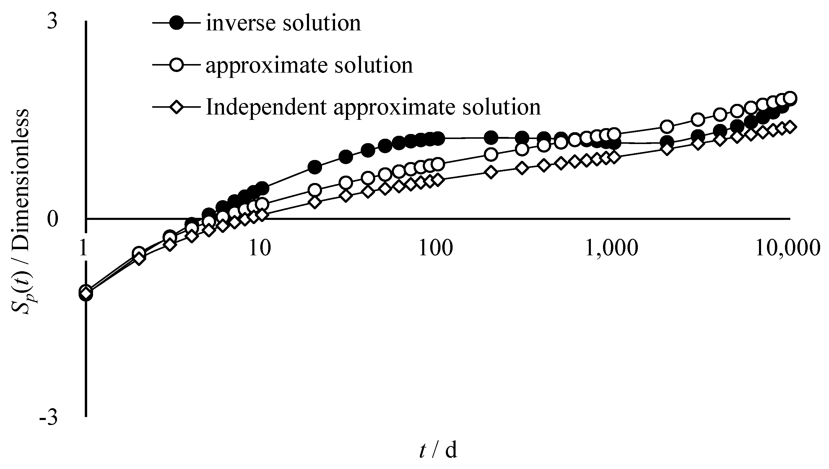
For a fixed-volume gas reservoir, a full-stage productivity equation has been created; continuous production and pressure are not required during the derivation process. Except for adding the pressure-conversion skin, the relevant stage was expanded from the stable production stage to the full gas reservoir development stage, compared to the quasi-steady-state production equation. The full-stage production-capacity equation was solved by building approximative and independent solutions for the pressure-conversion skin without influencing the addition of non-Darcy terms and the wellbore pressure drop skin.

(2)

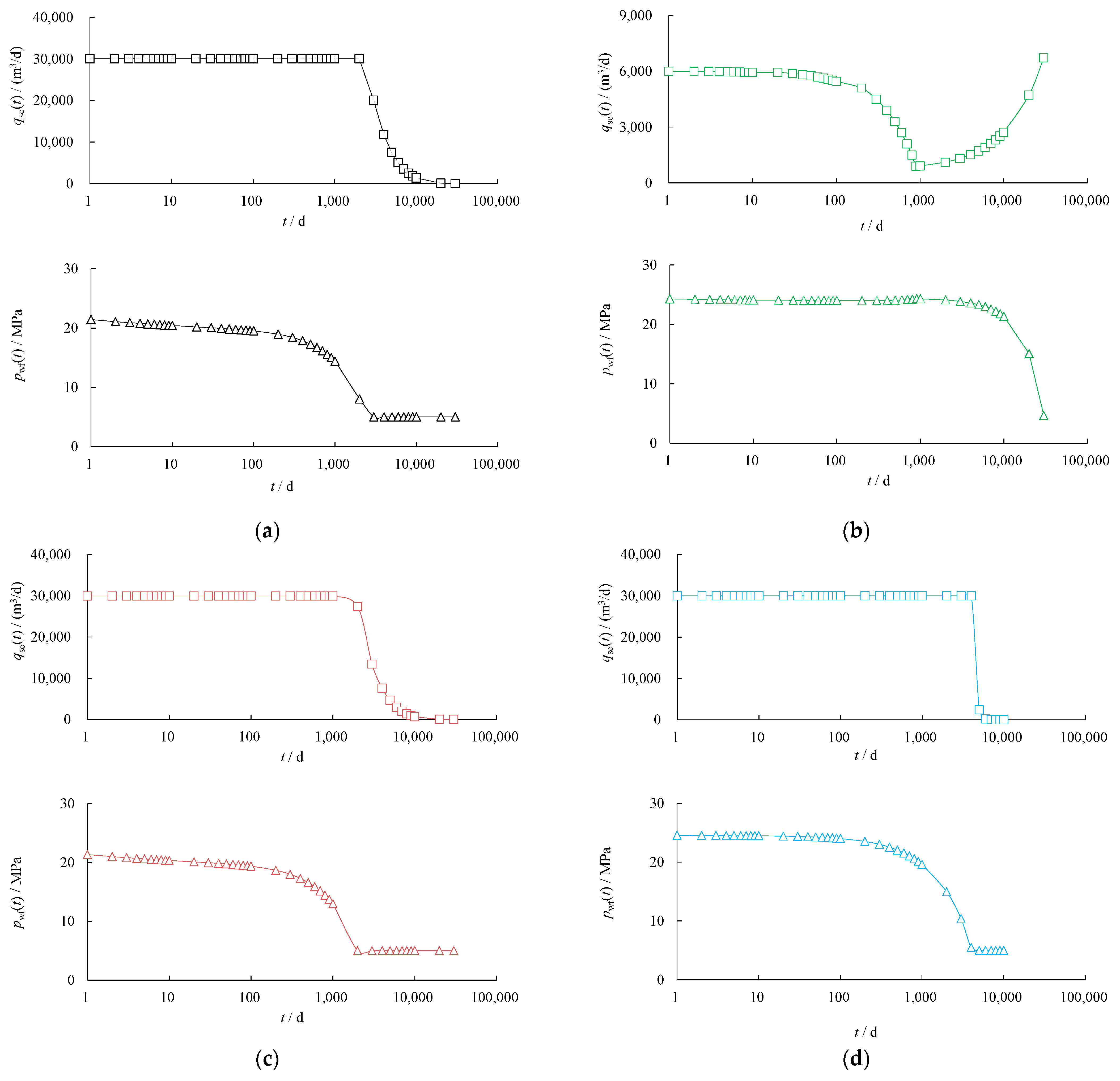
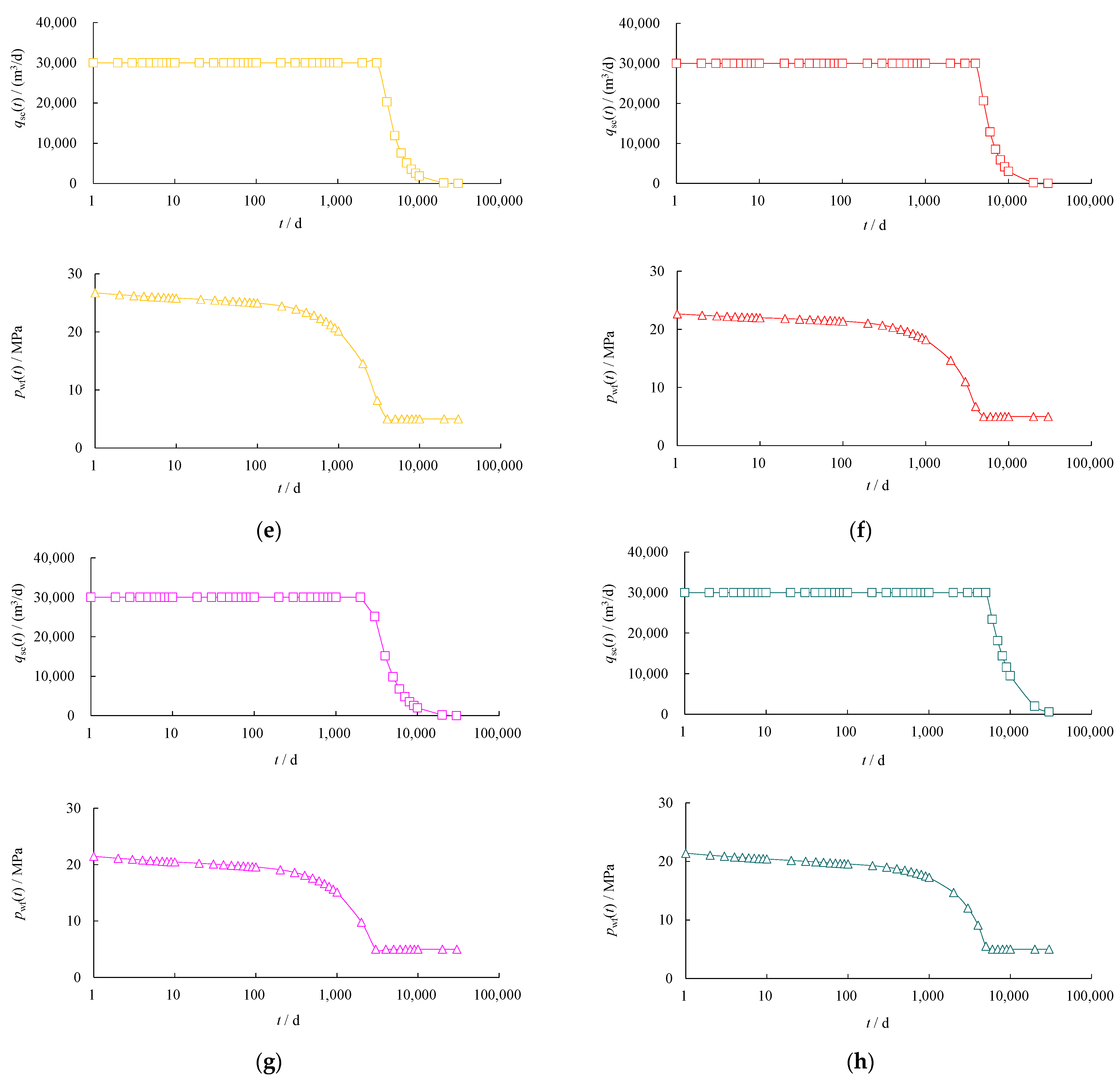
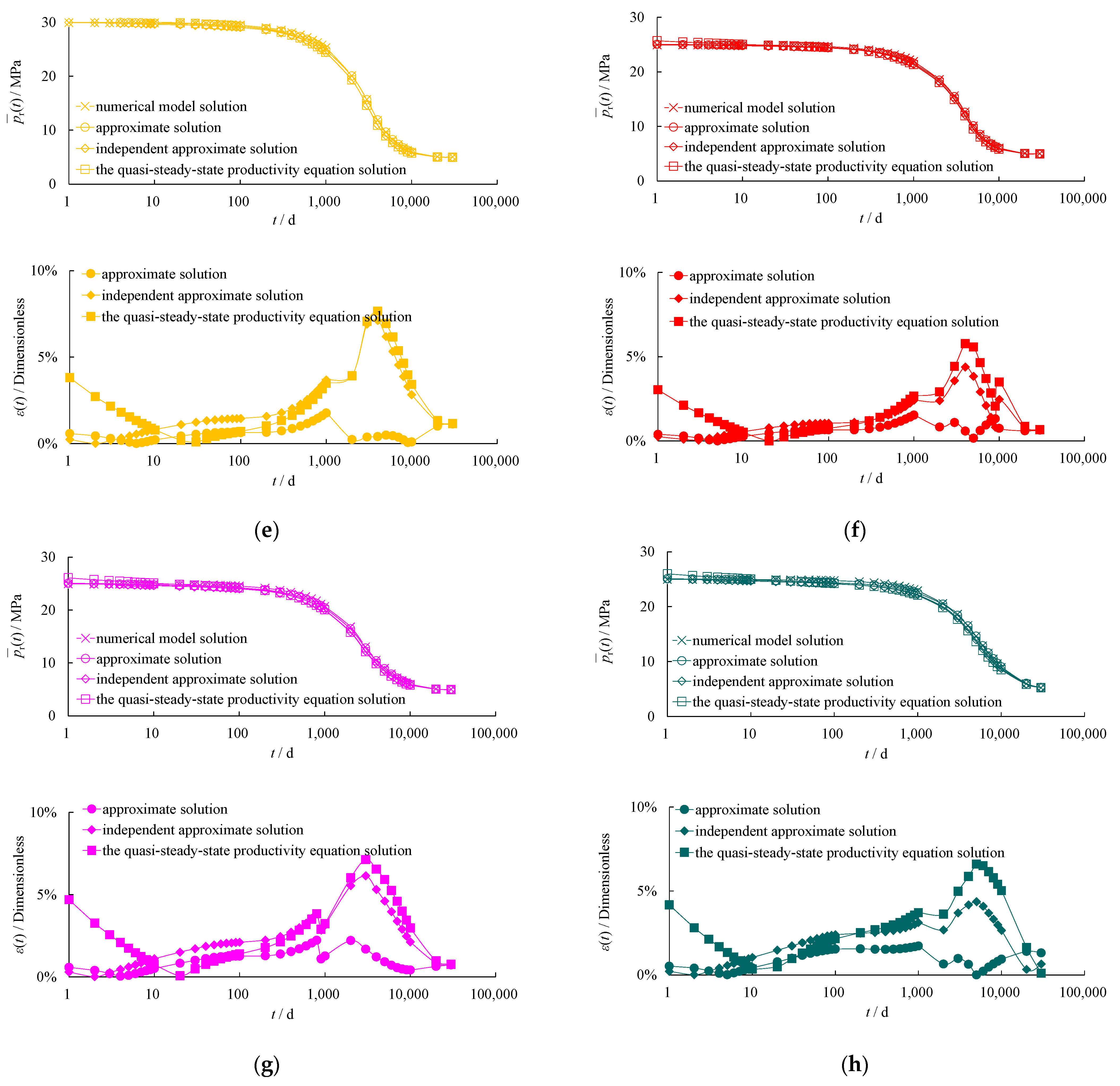
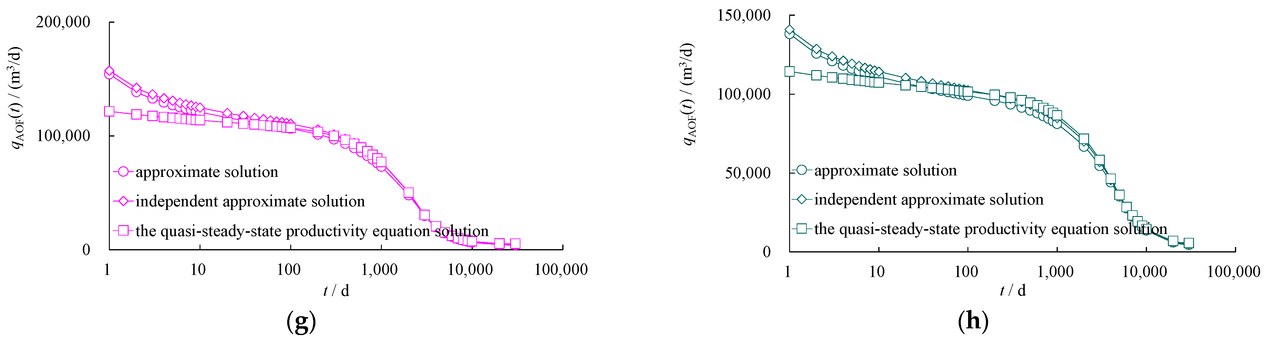
The approximate solution and independent approximate solution of the pressure-conversion skin are the only sources of error in the full-stage productivity equation. The validation of the model reveals that the approximate and independent solutions of the average formation pressure consistently exhibited good accuracy under varying production systems and fundamental factors. In contrast, the approximate and independent solutions of the absolute open-flow rate nearly overlap. The application results show that the full-stage productivity equation also has relatively reliable accuracy compared to the corrected isochronous well testing. The comprehensive model validation and application results indicate that the full-stage productivity equation is not affected by production systems, and this applies to the entire stage of gas reservoir development.

(3)

The precision of the approximation answer is marginally greater overall, and the effect of various pressure-conversion skins on the entire stage production-capacity equation varies. The independent approximation solution eliminates the effect of the venting radius. It is advised to utilize the approximate pressure-conversion skin solution for computing parameters like the average formation pressure. It is advised to utilize the independent approximation solution of the pressure-conversion skin to determine the absolute open-flow rate.

References

1. Guo, B.; Ghalambor, A. Natural Gas Engineering Handbook; Gulf Publishing Company: Houston, TX, USA, 2005; pp. 35–49. [Google Scholar]
2. Guo, C.; Li, F.; Liu, H.; Xia, Z.; Liu, X.; Fan, H.; Liu, L. Analysis of quantitative relationship between gas offtake and plateau duration of natural gas reservoir. Acta Pet. Sin. 2009, 30, 908–911. [Google Scholar]
3. Aminian, K.; Ameri, S.; Yussefabad, A.G. A simple and reliable method for gas well deliverability determination. In Proceedings of the SPE Eastern Regional Meeting, Lexington, KY, USA, 17–19 October 2007; SPE-111195-MS. SPE: Houston, TX, USA, 2007. [Google Scholar]
4. Li, S. Natural Gas Engineering, 2nd ed.; Petroleum Industry Press: Beijing, China, 2000; pp. 85–95. [Google Scholar]
5. Yang, J. Fundamentals of Gas Production Technology; Petroleum Industry Press: Beijing, China, 1992; pp. 44–58. [Google Scholar]
6. Cheng, Y.; Guo, C.; Tan, C.; Chen, P.; Shi, H.; Xing, Y. Experimental analysis and deliverability calculation of abnormally pressured carbonate gas reservoir considering stress sensitivity. J. Pet. Explor. Prod. Technol. 2022, 12, 3105–3115. [Google Scholar] [CrossRef]
7. Xiao, X.; Bi, Y.; Wang, X.; Gao, J.; Chang, Z.; Zhang, J. A new trinomial deliverability equation with consideration of stress sensitivity. Nat. Gas Geosci. 2014, 25, 767–770. [Google Scholar]
8. Al-Attar, H.; Al-Zuhair, S. A general approach for deliverability calculations of gas wells. In Proceedings of the SPE North Africa Technical Conference and Exhibition, Marrakech, Morocco, 12–14 March 2008; SPE-111380-MS. SPE: Houston, TX, USA, 2008. [Google Scholar]
9. Chen, Y. A simple method for determining absolute open flow rate of gas well. Nat. Gas Ind. 1987, 7, 59–63. [Google Scholar]
10. Kalantariasl, A.; Farhadi, L.; Farzani, S.; Keshavarz, A. A new comprehensive dimensionless inflow performance relationship for gas wells. J. Pet. Explor. Prod. Technol. 2022, 12, 2257–2269. [Google Scholar] [CrossRef]
11. Liang, H.; An, X.; Li, X. Principles for application of single point test and errors of deliverability evaluation of gas exploration well. Nat. Gas Ind. 2006, 26, 92–95. [Google Scholar]
12. Zhuang, H. Dynamic Description and Well Test of Gas Reservoirs; Petroleum Industry Press: Beijing, China, 2004; pp. 45–49. [Google Scholar]
13. Sun, H.; Meng, G.; Cao, W.; Su, X.; Liang, Z.; Zhang, R.; Zhu, S.; Wang, S. Applicable conditions of the binomial pressure method and pressure-squared method for gas well deliverability evaluation. Nat. Gas Ind. B 2020, 7, 397–402. [Google Scholar] [CrossRef]
14. Tan, Y.; Lian, L.; Yan, M. Calculation of pseudo pressure for real gas. Gas Heat 1999, 19, 31–33. [Google Scholar]
15. Tian, J.; Li, C.; Huang, S.; Li, D.; Jiang, Y. A new empirical formula of pseudo pressure calculation for real gas. Oil Drill. Prod. Technol. 2009, 31, 65–67. [Google Scholar]
16. Li, C.; Li, X.; Gao, S.; Liu, H.; You, S.; Fang, F.; Shen, W. Experiment on gas-water two-phase seepage and inflow performance curves of gas wells in carbonate reservoirs: A case study of Longwangmiao Formation and Dengying Formation in Gaoshiti-Moxi block, Sichuan Basin, SW China. Pet. Explor. Dev. 2017, 44, 930–938. [Google Scholar] [CrossRef]
17. Li, Y. An analysis of dimensionless IPR equations for gas wells. Nat. Gas Ind. 1995, 15, 48–53. [Google Scholar]
18. Wang, C.; Li, Z.; Lai, F. A novel binomial deliverability equation for fractured gas well considering non-Darcy effects. J. Nat. Gas Sci. Eng. 2014, 20, 27–37. [Google Scholar] [CrossRef]
19. Guo, P.; Wen, Y.; Wang, Z.; Ren, J.; Yang, L. An Unsteady-State Productivity Model and Main Influences on Low-Permeability Water-Bearing Gas Reservoirs at Ultrahigh Temperature/High Pressure. ACS Omega 2022, 7, 6601–6615. [Google Scholar] [CrossRef] [PubMed]
20. Osisanya, S.O.; Ayokunle, A.T.; Ghosh, B.; Suboyin, A. A modified horizontal well productivity model for a tight gas reservoir subjected to non-uniform damage and turbulence. Energies 2021, 14, 8334. [Google Scholar] [CrossRef]
21. Zhang, H.; Wang, L.; Wang, X.; Zhou, W.; Zeng, X.; Liu, C.; Zhao, N.; Wang, L.; Wang, X.; Wang, W. Productivity analysis method for gas-water wells in abnormal overpressure gas reservoirs. Pet. Explor. Dev. 2017, 44, 258–262. [Google Scholar] [CrossRef]
22. Kang, X.; Li, X.; Cheng, S. Evaluation of non-Darcy flow effect in gas well considering influence of flow boundary. J. China Univ. Pet. 2006, 30, 82–85. [Google Scholar]
23. Xue, J.; Zhang, M.; Song, H.; Wang, H. Multiple-factor Estimation for Productivity of Low Permeability Gas Reservoir. Sci. Technol. Eng. 2020, 20, 3940–3945. [Google Scholar]
24. Pan, Y.; Xu, Y.; Yang, Z.; Wang, C.; Liao, R. Shale gas productivity prediction model considering time-dependent fracture conductivity. Processes 2022, 10, 801. [Google Scholar] [CrossRef]
25. Xu, B.; Li, X.; Yin, B. Influence of gas slippage on gas well productivity evaluation. Nat. Gas Ind. 2010, 30, 45–48. [Google Scholar]
26. Yan, W.; Qi, Z.; Yuan, Y.; Li, J.; Huang, X. Productivity equation of low-permeability condensate gas well considering the influence of multiple factors. J. Pet. Explor. Prod. Technol. 2019, 9, 2997–3005. [Google Scholar] [CrossRef]
27. Chen, F.; Duan, Y.; Wang, K. Productivity Model Study of Water-Bearing Tight Gas Reservoirs Considering Micro-to Nano-Scale Effects. Processes 2024, 12, 1499. [Google Scholar] [CrossRef]
28. Li, M.; Xue, G.; Luo, B.; Yang, W. Pseudosteady-State Trinomial Deliverability Equation and Application of Low Permeability Gas Reservoir. Xinjiang Pet. Geol. 2009, 30, 593–595. [Google Scholar]
29. Wu, K.; Li, X.; Yang, P.; Zhang, S. The Establishment of a Novel Deliverability Equation of Abnormal Pressure Gas Reservoirs Considering a Variable Threshold Pressure Drop. Pet. Sci. Technol. 2014, 32, 15–21. [Google Scholar] [CrossRef]
30. Ghahri, P.; Alatefi, S.; Jamiolahmady, M. A new, accurate and simple model for calculation of horizontal well productivity in gas and gas condensate reservoirs. In Proceedings of the SPE Europec featured at EAGE Conference and Exhibition, Madrid, Spain, 1–4 June 2015; SPE-174345-MS. SPE: Houston, TX, USA, 2015. [Google Scholar]
31. Xie, X.; Luo, K.; Song, W. A novel equation for modeling gas condensate well deliverability. Acta Pet. Sin. 2001, 22, 36–42. [Google Scholar]
32. Ghahri, P.; Jamiolahmadi, M.; Alatefi, E.; Wilkinson, D.; Dehkordi, F.; Hamidi, H. A new and simple model for the prediction of horizontal well productivity in gas condensate reservoirs. Fuel 2018, 223, 431–450. [Google Scholar] [CrossRef]
33. Song, H.; Liu, Q.; Yang, D.; Yu, M.; Lou, Y.; Zhu, W. Productivity equation of fractured horizontal well in a water-bearing tight gas reservoir with low-velocity non-Darcy flow. J. Nat. Gas Sci. Eng. 2014, 18, 467–473. [Google Scholar] [CrossRef]
34. Yu, Q.; Jia, Y.; Liu, P.; Hu, X.; Hao, S. Rate transient analysis methods for water-producing gas wells in tight reservoirs with mobile water. Energy Geosci. 2024, 5, 100251. [Google Scholar] [CrossRef]
35. Zhang, J.; Gao, S.; Liu, H.; Ye, L.; Zhu, W.; An, W. Research on types of gas reservoirs divided by seepage capacity and their seepage mechanism, law and productivity. Energy Rep. 2023, 10, 2537–2550. [Google Scholar] [CrossRef]
36. Wang, Y.; Jiang, T.; Zeng, B. Productivity performances of hydraulically fractured gas well. Acta Pet. Sin. 2003, 24, 65–68. [Google Scholar]
37. Liu, S.; Xiong, S.; Weng, D.; Song, P.; Chen, R.; He, Y.; Liu, X.; Chu, S. Study on deliverability evaluation of staged fractured horizontal wells in tight oil reservoirs. Energies 2021, 14, 5857. [Google Scholar] [CrossRef]
38. Ehibor, L.; Ohenhen, L.; Oloyede, B.; Adetoyi, G.; Amaechi, T.; Olajide, O.; Kaka, A.; Woyengidiripre, A. Gas Condensate Well Deliverability Model, a Field Case Study of a Niger Delta Gas Condensate Reservoir. In Proceedings of the SPE Nigeria Annual International Conference and Exhibition, Lagos, Nigeria, 1–3 August 2022; 212043-MS. SPE: Houston, TX, USA, 2022. [Google Scholar]
39. Liu, Y.; Li, X.; Kang, X. Determination of reasonable pressure difference for condensate gas reservoir. Acta Pet. Sin. 2006, 27, 85–88. [Google Scholar]
40. Ogunrewo, O.; Herens, T.; Gringarten, A.C. Well deliverability forecasting of gas condensate and volatile oil wells below saturation pressure. In Proceedings of the SPE Europec featured at EAGE Conference and Exhibition, London, UK, 1–13 June 2013; SPE-164869-MS. SPE: Houston, TX, USA, 2013. [Google Scholar]
41. Wang, W.; Lei, X.; Lu, R.; Chen, J.; He, Z. Regional productivity prediction technology for abnormal high temperature and high pressure gas reservoirs in western south China sea. Earth Sci. 2019, 44, 2636–2642. [Google Scholar]
42. Wang, F.; Liu, S.; Jia, Y.; Gao, A.; Su, K.; Liu, Y.; Du, J.; Wang, L. Production forecasting methods for different types of gas reservoirs. Energy Geosci. 2024, 5, 100296. [Google Scholar] [CrossRef]
43. Du, X.; Zhang, Y.; Zhou, C.; Su, Y.; Li, Q.; Li, P.; Lu, Z.; Xian, Y.; Lu, D. A novel method for determining the binomial deliverability equation of fractured caved carbonate reservoirs. J. Pet. Sci. Eng. 2022, 208, 109496. [Google Scholar] [CrossRef]
44. Hu, J.; Yang, S.; Wang, B.; Yan, Y.; Deng, H.; Zhao, X. Trinomial capacity equation for horizontal wells in deep carbonate gas reservoirs: Case study of Dengying Formation in Anyue Gas Field, Sichuan Basin. Nat. Gas Geosci. 2023, 34, 1112–1122. [Google Scholar]
45. Li, Y.; Feng, Y.; Li, X.; Zhong, J.; Wang, W. Productivity performance of open hole horizontal gas well for low permeability gas reservoirs. Pet. Sci. Technol. 2024, 42, 169–189. [Google Scholar] [CrossRef]
46. Wei, B.; Nie, X.; Zhang, Z.; Ding, J.; Shayireatehan, R.; Ning, P.; Deng, D.; Cao, Y. Productivity Equation of Fractured Vertical Well with Gas–Water Co-Production in High-Water-Cut Tight Sandstone Gas Reservoir. Processes 2023, 11, 3123. [Google Scholar] [CrossRef]
47. Zhu, W.; Song, H.; He, D.; Wang, M.; Jia, A.; Hu, Y. Low-velocity non-Darcy gas seepage model and productivity equationsof low-permeability wate-|bearing gas reservoirs. Nat. Gas Geosci. 2008, 19, 685–689. [Google Scholar]
48. Zeng, D.; Zhang, Q.; Li, T.; Su, Y.; Zhang, R.; Zhang, C.; Peng, S. Key technologies for long-period high and stable production of the Puguang high-sulfur gas field, Sichuan Basin. Nat. Gas Ind. 2023, 43, 65–75. [Google Scholar]
49. Li, G.; Wu, X.; Llt, Y.; Yang, J. Full life-circle production and elfect evaluation of Panzhuang coalbed meth-ane wells in 0inshui Basin. J. China Coal Soc. 2020, 45, 894–903. [Google Scholar]
50. Gao, S.; Liu, H.; Ye, L.; Hu, Z.; An, W. Physical simulation experiment and numerical inversion of the full life cycle of shale gas well. Acta Pet. Sin. 2018, 39, 435–444. [Google Scholar] [CrossRef]
51. Mehrdad, V.; Rasa, S.; Saeid, J.; Saeed, S. Development of a dynamic model for drilling fluid’s filtration: Implications to prevent formation damage. In Proceedings of the SPE International Conference and Exhibition on Formation Damage Control, Lafayette, LA, USA, 26–28 February 2014; SPE-168151-MS. SPE: Houston, TX, USA, 2014. [Google Scholar]
52. Salehi, S.; Hussmann, S.; Karimi, M.; Ezeakacha, C.; Tavanaei, A. Profiling drilling fluid’s invasion using scanning electron microscopy: Implications for bridging and wellbore strengthening effects. In Proceedings of the SPE Deepwater Drilling and Completions Conference, Galveston, TX, USA, 10–11 September 2014; SPE-170315-MS. SPE: Houston, TX, USA, 2014. [Google Scholar]
53. Ezeakacha, C.P.; Salehi, S.; Hayatdavoudi, A. Experimental study of drilling fluid’s filtration and mud cake evolution in sandstone formations. J. Energy Resour. Technol. 2017, 139, 022912. [Google Scholar] [CrossRef]
54. Vasheghani, F.M.; Foroughi, S.; Norouzi, S.; Jamshidi, S. Mechanistic study of fines migration in porous media using lattice Boltzmann method coupled with rigid body physics engine. J. Energy Resour. Technol. 2019, 141, 123001. [Google Scholar] [CrossRef]
Figure 1. Typical inverse solutions, approximate solutions, and independent approximate solutions of Sp(t).
Processes 12 01855 g001
Figure 2. PVT and phase permeability in mathematical modeling.
Processes 12 01855 g002
Figure 3. qsc(t) and pwf(t) output from numerical simulation. (a) Model 1. (b) Model 2. (c) Model 3. (d) Model 4. (e) Model 5. (f) Model 6. (g) Model 7. (h) Model 8.
Processes 12 01855 g003aProcesses 12 01855 g003b
Figure 4. Comparison of p ¯ r ( t ) calculated in different ways. (a) Model 1. (b) Model 2. (c) Model 3. (d) Model 4. (e) Model 5. (f) Model 6. (g) Model 7. (h) Model 8.
Processes 12 01855 g004aProcesses 12 01855 g004b
Figure 5. Comparison of qAOF(t) calculated in different ways. (a) Model 1. (b) Model 2. (c) Model 3. (d) Model 4. (e) Model 5. (f) Model 6. (g) Model 7. (h) Model 8.
Processes 12 01855 g005aProcesses 12 01855 g005b