A New Monitoring Method for the Injection Volume of Blast Furnace Clay Gun Based on Object Detection

Abstract

Monitoring the injection volume of clay guns is important in blast furnace ironmaking. Currently, such monitoring data are often recorded manually, which has limitations such as low reliability and high delay. To address these issues, we revisit the task from a computer vision perspective and propose an object detection method. First, we introduce an interpolation annotation technique to build a clay gun dataset. With it as a foundation, an improved object detection model called Faster R-CNN with multi-stage Positional encoding and two-branch Self Challenge (PSCfrcn) is proposed. Our model leverages multi-stage positional encoding (PE) to focus more on the relative position of local features, and a self-challenge (SC) module to mitigate the interference caused by the harsh environments. We conduct extensive experiments on the clay gun dataset from actual industrial scenarios, and use various metrics to validate the performance. Experimental results demonstrate that our method can significantly enhance the model’s discriminative power and generalization ability, which is a promising direction for this task.

1. Introduction

As a key equipment for ironmaking, the blast furnace (BF) generally has multiple tapholes. Since hot metal is periodically discharged through different tapholes, each taphole undergoes a cycle of opening and closing [1,2,3]. After tapping, the taphole is sealed with clay using a clay gun, forming a clay bulge in the taphole as shown in Figure 1. Accurately measuring the volume of clay extruded from the clay gun is crucial for ensuring a solid seal. Injecting too much clay can result in a taphole that is too deep, delaying hot metal discharge and impacting production. Conversely, insufficient clay may lead to the thinning of the furnace wall due to excessive iron flow, which can reduce the BF lifespan. Inadequate sealing also compromises the taphole’s quality and affects subsequent openings. Therefore, the precise monitoring of the clay gun’s injection volume is essential.

Although some methods [4,5,6,7,8,9] have been proposed for monitoring the injection volume of the clay gun, each has their own shortcomings. In practice, manually observing the vernier’s position remains the most widely used approach. However, poor visibility caused by smoke and dust around the taphole presents a challenge. Additionally, variations in operators’ skills and experience can lead to differing perspectives when viewing the vernier and scales, resulting in inconsistent readings. As a result, the clay injection volume is often determined by the operator’s subjective judgment [7].

In Figure 2, image (a) depicts the scene of a BF clay gun in operation. Once the clay gun is positioned at the taphole, clay is extruded to securely seal it. As the amount of injected clay increases, the machine’s vernier at the tail end rises accordingly. In the enlarged Figure 2b, we highlight the vernier with a red dashed box and use yellow lines to emphasize the different scales.

What makes the detection more complex is that various adverse conditions widely exist, which will easily lead to detection errors. Figure 2c shows the situation where the vernier may sway during the machine’s operation. Figure 2d illustrates poor lighting. Especially at the beginning of clay injection, the site’s lighting is usually obstructed by dust particles, affecting the camera’s ability to capture the scene. Figure 2e shows water vapor rising. In such a high-temperature environment, the water vapor often obstructs the clay gun. Therefore, choosing the right model and making task-specific improvements to adapt to the various adverse factors require careful consideration.

To address this problem, we propose an object detection model called Faster R-CNN with multi-stage Positional encoding and two-branch Self-Challenge (PSCfrcn). By framing the problem as an object detection task, we can accurately detect the vernier and scale regions, allowing for the prediction of the vernier’s position through feature extraction and classification. Specifically, since the determination of the clay injection volume relies on the relative position between the vernier and various scales, we designed a multi-stage positional encoding (PE) to enhance the model’s sensitivity to feature positions, thus improving classification accuracy. Additionally, to mitigate interference from the harsh environments mentioned earlier, we adapted the self-challenge (SC) method, originally intended for classification tasks, for our object detection model. This adjustment enhances the model’s generalization ability by suppressing certain features during the training phase. The contributions of this article are as follows.

• This is the first time the task of monitoring the injection volume of a BF clay gun has been approached using computer vision. We propose a comprehensive solution, from data collection to model implementation, offering a novel perspective for future researchers.
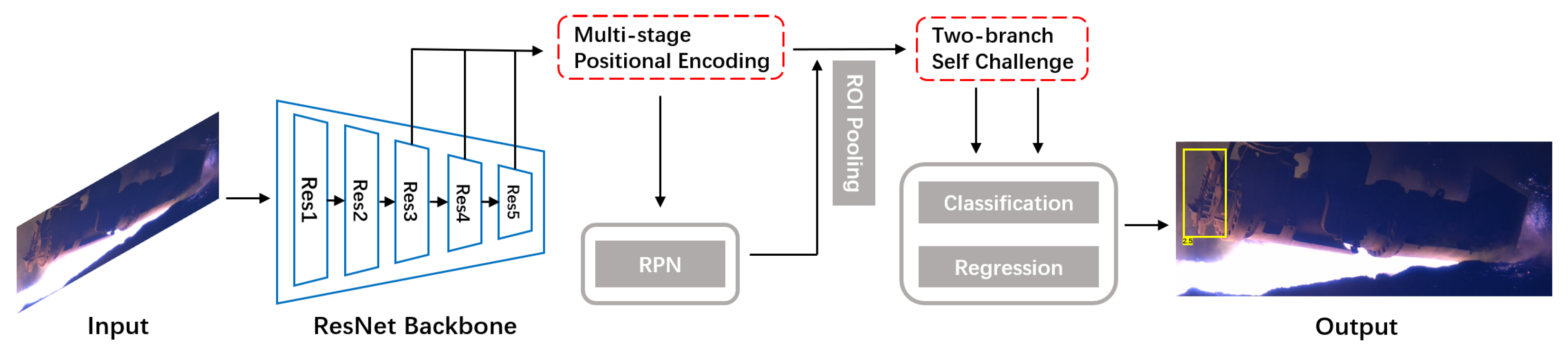
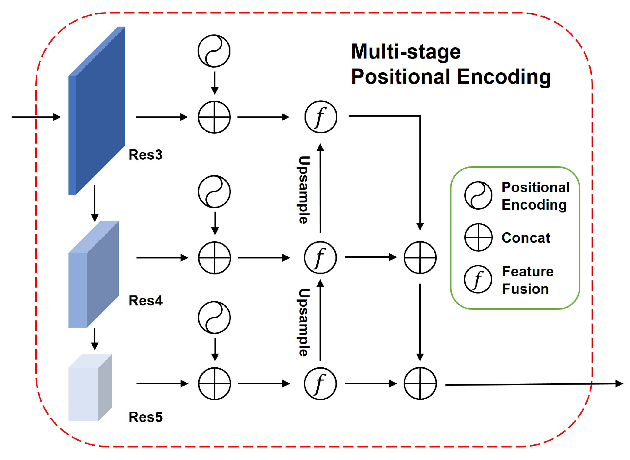
• We propose PSCfrcn, composed of multi-stage positional encoding and two-branch self-challenge, which consistently improves the accuracy and stability of the objective detection model for the problem we address.
• We conduct extensive experiments on the clay gun dataset from actual industrial scenarios, and use various metrics to validate the performance improvements brought by our model.

In the following parts of this paper, we commence by introducing related work and then delve into data collection and annotation. After carefully choosing the baseline, we elaborate on our innovations, the multi-stage PE and two-branch SC. Subsequently, through experiments, we compare our proposed PSCfrcn model with existing methods, clearly demonstrating its superiority. Finally, we conduct comprehensive ablation experiments to analyze the improvement of each module and the parameter settings.

2. Related Work

2.1. Injection Volume Monitoring of Clay Gun

There are three common methods for monitoring the injection volume of a clay gun: timing the injection, measuring the clay weight, and observing the vernier. The first method uses a stopwatch to control the injection time, estimating the volume based on duration. However, since the injection rate varies with the taphole’s condition, this approach is often inaccurate. The second method involves weighing the clay before loading it into the clay gun, but it requires precise prediction of the clay consumption and lacks flexibility in handling on-site abnormalities. The most widely used method is manually observing the vernier’s position, though this is prone to subjectivity due to poor visibility and variations in operators’ skills and experience.

Recently, some research studies have also explored intelligent technology for monitoring the clay injection volume, which primarily focuses on sensors or flow meters. In [4,5], they install linear displacement sensors at the end of the hydraulic clay injector, allowing the calculation of clay injection volume through programming, while [6] installs turbine flow sensors and accompanying calculation instruments in the hydraulic circuit of the rod chamber of the clay gun to measure the volume. Unlike the aforementioned work, refs. [7,8,9] modify the hydraulic control circuit by installing flow meters for the hydraulic oil pump’s discharge so as to calculate the clay injection volume indirectly. However, all these equipment and their auxiliary transmission devices have to be installed on the clay gun or near the taphole that is under high temperature, pressure, steam and dust. Due to long-term exposure to such typical harsh environments, the above-mentioned equipment is hard to widely applied in practice and easily damaged.

2.2. Object Detection

Object detection is a computer vision task whose goal is to detect and locate objects of interest in an image or video. The task involves identifying the position and boundaries of objects in an image, and classifying the objects into different categories. Over time, object detection models have evolved into one-stage and two-stage detectors, each with its advantages and limitations [10].

One-stage methods aim to directly predict the class and location of objects. Among the prominent examples of one-stage techniques is the YOLO (You Only Look Once) series [11,12], which uses a single Convolutional Neural Network (CNN) to achieve end-to-end object detection. Instead of using the anchor box as prior knowledge, CornerNet [13] calibrates the position of objects through diagonal points, which not only simplifies the model structure, but also reduces the complexity of the regression process. By adding a center point, CenterNet [14,15] detects each object as a triplet keypoint, which can locate objects with arbitrary geometries and perceive the global information of objects. The advantage of one-stage methods is their speed and simplicity, though they usually have lower accuracy compared to two-stage detectors, especially for small or occluded objects.

By contrast, the two-stage methods handle object detection in two steps: localization followed by classification. As a typical method of two-stage method, Faster R-CNN [16] introduces the Region Proposal Network (RPN) to generate candidate regions, which significantly optimizes the speed and accuracy of two-stage object detection. To address the challenge of detecting objects with significant size differences, FPN [17] introduced a feature pyramid network structure, which effectively handles multi-scale variations. Unlike RPN which generates prior boxes through anchors, the corner proposal network (CPN) [18] employs a corner pairing method similar to CenterNet and CornerNet to locate the classification targets. It possesses the capability to detect targets of arbitrary geometric shapes and capture global information within them, thereby effectively reducing the number of false positive samples.

Most existing object detection models use CNNs (e.g., ResNet and Darknet) for feature extraction. Compared to CNNs, Transformers offer a larger receptive field, more flexible weight configuration and superior global feature modeling capabilities. Recently, some studies have proposed object detection methods based on transformers. To reduce reliance on prior designs in the label assignment process, DETR (Detection Transformer) [19] redefines object detection as a set prediction problem. By predicting a set encompassing all targets in a single step, it achieves end-to-end training. Building upon DETR, many research studies have followed up [20,21,22,23]. As one of the most recent studies, ref. [24] propose the first real-time end-to-end DETR object detector (RT-DETR) which can improve speed by decoupling intra-scale inter action and cross-scale fusion. Some research studies propose a Transformer-based general-purpose backbone, such as Vision Transformer (ViT) [25] and Swin Transformer (Swin-T) [26]. However, Transformer-based object detection methods are generally computationally intensive, which requires high computational cost, large memory consumption, and a large amount of labeled data.

Most existing objective detection models are validated on standard image datasets like PASCAL VOC and MS COCO, which consist of relatively clear images. In contrast, our images contain significant noise due to harsh working conditions, including high temperatures, dust, and water vapor. This is the first attempt to apply object detection to the task of monitoring the injection volume of a clay gun, requiring a systematic design from data collection to model implementation, presenting considerable challenges.

3. Data Collection and Annotation

Recently, the furnace front monitoring system has been widely used, which uses cameras installed on factory walls or pillars to record the real-time furnace front operations. Through such a system, we can obtain the video recording of the whole process of the clay gun operation. In our experiment, the images are captured from the No.7 BF (1750 m³ in volume) at Tranvic Steel Co., Ltd., Neijiang, Sichuan, China, an example of which is shown in Figure 2a. By collecting videos with various vernier positions under different working conditions, we can construct a dataset for our object detection task.

The next step is annotation. In line with the object detection methods, we need to define the bounding box and label for each image. Since our area of interest is the vernier and the scales at the tail of the clay gun, the vernier and scale region is enclosed within a bounding box as illustrated in Figure 2a. We then assign a label based on the vernier’s position. For instance, in Figure 2a, the label is 2, as the vernier is aligned with the second scale. However, due to the narrow intervals and fuzzy boundaries between adjacent scales, manually classifying and labeling the images can be challenging, especially for non-integer categories. Given that the vernier moves nearly linearly during operation, we employ a linear interpolation method for data annotation to address this difficulty.

The image sequence of a clay gun operation video is taken as input. We first manually label the images in which the vernier is at integer scale (e.g., 1 and 2) or half scale (e.g., 1.5, 2.5). Then, we divide the frames evenly between the adjacent scales into four parts so as to obtain the intermediate categories. For example, the images between the labels 1 and 1.5 are divided so that each parts are automatically assigned with labels of 1.1 to 1.4, respectively. Through such an approach, we elegantly solve the labeling issue of intermediate scale categories regarding the dataset for this task.

4. Our Model

The overview of our model is shown in Figure 3. We incorporate our improvements into a vanilla Faster R-CNN. After extracting the raw image features with the ResNet backbone, we introduce multi-stage positional encoding to enhance the model’s focus on the spatial information of local features. Moreover, we apply our two-branch self-challenge to Region of Interest (ROI) pooling outputs, adjusting the model’s training on local features by leveraging the back propagation gradients and outputs of the last layer.

We adopt the same training method as Faster R-CNN [16]. The objective loss function is mainly divided into the loss of the RPN and the loss of the R-CNN. Moreover, both parts of the loss include the classification loss and the regression loss, which are calculated using the cross-entropy loss and the smooth L1 loss, respectively. The overall model is jointly optimized by minimizing a unified objective function as shown in Equation (1):

$${\mathcal{L}}_{total}=({\mathcal{L}}_{rpn}^{cls}+{\lambda }_{rpn}·{\mathcal{L}}_{rpn}^{reg})+\eta ·({\mathcal{L}}_{rcnn}^{cls}+{\lambda }_{rcnn}·{\mathcal{L}}_{rcnn}^{reg})$$

(1)

Among them, $\lambda$ and $\eta$ are hyperparameters used to balance the losses of each part.

In the rest of this section, we first analyze the performance of different models on this task and explain why we select a two-stage object detection model as our baseline in Section 4.1. Then, we propose multi-stage PE and two-branch SC in Section 4.2 and Section 4.3 to enhance the model’s discrimination and generalization abilities, respectively.

4.1. Basic Model Selection

The goal of this section is to select a suitable baseline for our task, ensuring that our method appears complete and clear. In practice, we conduct extensive attempts with robust analysis and justification during this process. For the convenience of discussion, we present the results using representative algorithms of YOLOX and Faster R-CNN in Figure 4, while the remaining detailed experimental results and analysis are presented in Section 5.3. We test these two pre-trained models with our validation dataset and select three representative results for clear comparison.

Figure 4 shows the predicted positions of the vernier during the clay gun working. Since clay is continuously injected into the taphole, the vernier should consistently maintain a non-decreasing state. As shown in Figure 4, although both lines are on an upward trend, the performance of the YOLO model is generally inferior to that of frcn. Poor working conditions like vernier shaking, dim light, and mist result in worse model recognition performance which is manifested in the violent shaking of the polygonal line. Compared to YOLO, the two-stage frcn method has more accurate recognition in harsh environments, even if the line wobbles a little, and its amplitude is relatively small.

Compared to one-stage methods, two-stage ones use a Region Proposal Network (RPN) to preliminarily distinguish foreground objects from the background, and then perform fine classification and bounding box regression in the second stage, thus improving accuracy. Due to the noise such as mist and vernier vibrations, keeping high accuracy under various adverse conditions is the most challenging in our detection task. Therefore, a two-stage approach is preferred. Furthermore, given that the target size is relatively fixed and regular, multi-scale structures and keypoint detection fail to leverage their advantages and instead increase detection difficulty under challenging conditions. Thus, we follow the typical two-stage model Faster R-CNN as the baseline.

However, Faster R-CNN still encounters conflicts due to the joint optimization between class-agnostic RPN and class-relevant RCNN through the shared backbone. These mismatched goals may result in diminished classification performance. To solve this issue, the Gradient Decoupled Layer (GDL) is proposed in DeFRCN [27]. It can be inserted between the shared backbone and RPN; meanwhile, between the backbone and RCNN to adjust the degree of decoupling among three modules. Thus, to build a strong baseline, we equip Faster R-CNN with GDL to decouple the RPN and RCNN parts.

4.2. Multi-Stage PE

In our task, distinguishing between different categories is essentially based on the relative position of the vernier to different scales. To enable the model to infer the category according to the location of the vernier, we propose a multi-stage PE method as shown in Figure 5.

In NLP models like Transformer [28], positional encoding (PE) provides the position information of each token within a sentence. Inspired by this method, we also use sine and cosine functions for the position encoding of each local descriptor in the feature maps. Here, we take the channel of the feature maps as the dimension of each positional encoding. The sine and cosine PE functions of each local descriptor are calculated by Equations (2) and (3). We adopt the 2D positional encoding implementation from MAE [29], which involves adding PE separately in the height (H) and width (W) directions and then concatenating them. Thus, the position encoding of the feature maps is a 3D sin-cos tensor of the same size as the feature maps:

$$\begin{array}{cc}\hfill & P{E}_{(pos,2i)}=sin(pos/{10,000}^{2i/C})\hfill \end{array}$$

(2)

$$\begin{array}{cc}\hfill & P{E}_{(pos,2i+1)}=cos(pos/{10,000}^{2i/C})\hfill \end{array}$$

(3)

where $P{E}_{(pos,2i)}$ and $P{E}_{(pos,2i+1)}$ are the position encoding of an arbitrary local feature descriptor $P{E}_{\left(pos\right)}$. $pos=0,\dots ,H\times W$, where H and W are the height and width of the feature maps, respectively. $i=0,\dots ,C/2-1$, where C is the channel of the feature maps.

Thanks to this positional encoding, the position of any local feature can be precisely represented, allowing for easy computation of the relative positions of different local feature descriptors. Moreover, this positional encoding shares the same dimension as the feature maps, enabling the two to be summed together. This fusion effectively combines the embeddings of both the features and their corresponding positions.

It is important to note that our model utilizes ResNet as the backbone, which comprises five stages. Inspired by the pyramid structure of FPN [17], the corresponding positional encoding (PE) can be derived for each stage. Through experimentation, we discover that combining the last three stages with PE yields the best performance for our task. Consequently, we inject PE into the outputs of these last three stages. Additionally, the combined features in different scales are fused with each other through upsampling, which unifies the feature outputs of high-level and low-level stages, providing a position-aware input for subsequent modules. The process of the multi-stage feature fusion with PE can be given by Equations (4)–(7):

$$\begin{array}{c}{\Phi }_{Bloc{k}_i}=Re{s}_i\oplus P{E}_i\hfill \end{array}$$

(4)

$$\begin{array}{c}{f}_{Block4}={\Psi }_{up}\left({\Phi }_{Block5}\right)+{\Phi }_{Block4}\hfill \end{array}$$

(5)

$$\begin{array}{c}{f}_{Block3}={\Psi }_{up}\left({\Phi }_{Block4}\right)+{\Phi }_{Block3}\hfill \end{array}$$

(6)

$$\begin{array}{c}{f}_{output}={\Phi }_{Block5}\oplus f_{Block4}\oplus f_{Block3}\hfill \end{array}$$

(7)

where ${\Phi }_{Bloc{k}_i}$ represents the output of the ResNet $Re{s}_i$ combined with the positional encoding $P{E}_i$ in the ith stage. ${\Psi }_{up}(·)$ represents upsampling and ⊕ is matrix concat. Note that we have also experimented with trainable positional encoding like ViT, but since it increases the training burden without providing any improvement, we opt for this constant form instead.

4.3. Two-Branch SC

The three adverse conditions mentioned earlier can actually be summarized as image blurring and key region occlusion. Therefore, we use self-challenge mask to suppresses the network’s overemphasis on specific features during training, allowing the model to have a certain tolerance for object recognition, such as vernier deformation caused by shaking. Consider that our problem involves both classification and regression tasks, we propose a two-branch SC method.

The core idea of our two-branch SC module is to identify the most predictive subset of the features z and deactivates it, where a mask is used to adaptively control the feature selection during iterations. As depicted in Figure 6, after obtaining the ROI features, we generate self-challenge masks for both the classification and regression branches. These masks are then adjusted through batch dropout operation. Finally, we apply a Hadamard product between the modified masks and the ROI features, producing outputs that are fed into the last layer of Faster R-CNN.

In this paper, we follow the locate strategy in [30] to calculate the gradient of the upper layers (i.e, the ResNet backbone and multi-stage positional encoding) so as to generate the self-challenge masks for classification and regression branches. Next, the batch dropout operation runs as follows.

For classification branch, we first compute the output of the classification branch $h^c(z;{\theta }_t^c)$ using the feature representation z (or Z) learned by the backbone along with the ROI pooling. And then, we run softmax function to obtain the probabilities of each class as shown in Equation (8). Similarly, we compute another output using the feature representation $\widetilde{z^c}$ after part of the features are discarded by classification masks, and run softmax function to obtain their probabilities as shown in Equation (9). Next, we calculate the classification probability differences for the correct class and use it as the impact measure as shown in Equation (10):

$$\tilde{s}=softmax\left(h^c(z;{\theta }_t^c)\right)$$

(8)

$${\tilde{s}}^{\prime }=softmax\left(h^c({\tilde{z}}^c;{\theta }_t^c)\right)$$

(9)

$$im{p}^c=\sum \tilde{s}\odot y^c-\sum {\tilde{s}}^{\prime }\odot y^c,$$

(10)

where ${\theta }_t^c$ are the parameters of the last layer of the classification breach in the $t^{th}$ iteration. ⊙ denotes the Hadamard product. $im{p}^c$ denotes the classification impact. $y^c$ represents the one hot ground truth class.

At last, with the batch percentage $p^c$, we can compute the ${(100-p^c)}^{th}$ percentile, denoted as $q^c$ and modify masks for the classification branch $m^c$ by Equation (11):

$${m^c\left(i\right)}^{\prime }=\left\{\begin{array}{cc}{m}^c\left(i\right),\hfill & \mathrm{if}im{p}^c\left(i\right)\ge q^c\hfill \\ 1,\hfill & \mathrm{otherwise}.\hfill \end{array}\right.$$

(11)

For the regression branch, we have to calculate the bounding box offsets, which is quite different from the classification branch. Thus, we formulate a new expression by Equations (12) and (13), and utilize Equation (14) to compute the impact for the regression branch. After that, we also use Equation (11) to adjust its mask $m^b$, where all the variables with superscript symbol c is replaced by b:

$$\tilde{d}=h^b(z;{\theta }_t^b)\odot y^c$$

(12)

$${\tilde{d}}^{\prime }=h^b({\tilde{z}}^b;{\theta }_t^b)\odot y^c$$

(13)

$$im{p}^b=\sum |\tilde{d}-{\tilde{d}}^{\prime }|,$$

(14)

where $\widetilde{z^b}$ is the feature representation after part of the features are discarded by the regression mask. ${\theta }_t^b$ are the parameters of the last layer of the regression breach in the $t^{th}$ iteration. $im{p}^b$ denotes the regression impact.

We summarize our two-branch SC in Algorithm 1. We set the same batch percentage p for both of the branches because [30] find that the variation of this hyperparameter has little effect on the results and fix it as a constant in their classification task. Since object detection models differentiate the background class, we exclude this class’s backward gradient impact for two-branch SC. Note that the new formulas are specifically designed for the regression branch of object detection without altering other components, ensuring that no new parameters need to be introduced for training.

Algorithm 1 Two-branch SC.

Input: Dataset $\langle X,Y\rangle$, percentage of batch to modify p, maximum number of epoches T, ROI features Z; Output: Last layer of our model $f(·;{\theta }_{t+1})$;  Random initialize the model ${\theta }_0$;  while$t\le T$ do   for every batch $x,y$ do    Generate $m^c$ and $m^b$ by the locate strategy [30];    if $p\ne -1$ then                    ▹ Use batch dropout     Calculate the probabilities by Equations (8) and(9);     Calculate the classification impact by Equation (10);     Calculate the offsets by Equations (12) and (13);     Calculate the regression impact by Equation (14);     Update ${m^c}^{\prime }$ and ${m^b}^{\prime }$ by Equation (11);    end if    Obtain classification features $Z^c={m^c}^{\prime }\odot Z$ and regression features $Z^b={m^b}^{\prime }\odot Z$;    Update $f(·;{\theta }_{t+1})$ by the gradient of the model;   end for  end while

5. Method Validation

5.1. Data Preparation

To validate the effectiveness of the model, we capture 20 BF clay gun videos in No.7 BF (1750 m³ in volume) at Tranvic Steel Co., Ltd., which cover different operational durations under various working conditions. We do not selectively choose images from the video; instead, we directly convert the video into dataset images by fixed interval frame sampling. This ensures that our interpolation labeling method can be effectively applied to our dataset. The annotated VOC image dataset is then split into training and validation sets in a 4:1 ratio, with the division performed at the video level. This helps avoid inflated test results due to similar environmental conditions in the same clay gun operation. Since the challenging conditions including mist, vernier vibrations, and varying lighting conditions are widespread and randomly distributed throughout our dataset, we ensure that our experiments can comprehensively evaluate the models’ performance under complex working conditions.

To ensure a fair comparison, all detectors are trained on one Tesla V100, 32G with Intel Xeon 6 Series, 12 Core. The original image size is $1920\times 1080$, but the clay gun always occupies only the upper half of the image. Then, we preprocess the images by cropping them, allowing us to set the batch size to 8. We also apply simple data augmentation methods, such as flipping and adjusting brightness. Furthermore, the detectors are optimized using SGD with a learning rate of 0.02, a momentum of 0.9, and a weight decay of 0.0001. The 2k and 1k region proposals are generated with a non-maximum suppression threshold of 0.7 for training and inference phase. In each training step, 512 proposals are sampled from 2k proposals as the box candidates to train RCNN.

5.2. Evaluation Metrics

Note that the injection volume of the clay gun is output by the classification result of our object detection model, in which we use different categories to represent vernier’s position. To intuitively assess the results for our task, we use accuracy—the ratio of correctly predicted samples to the total number of samples—as one of the evaluation metrics. The accuracy focuses on the correctness of classification rather than the precision of the bounding boxes, making it a valuable reference in our predominantly classification-oriented task.

Besides that, we take mAP (mean Average Precision), which is commonly used for object detection tasks, as the metric to evaluate our model. Specifically, we use IoU (Intersection Over Union) to determine whether the predicted boxes are accurate. Once the labeling is complete, the recall (R in Equation (16)) will always rise. And then, we employ the interpolation approximation method to average the precision (P in Equation (15)) across various recall levels, resulting in the Average Precision (AP in Equation (17)). Finally, we average the AP across all classes according to their proportions to obtain the mAP metric as Equation (18):

$$\begin{array}{cc}\hfill & P=TP/(TP+FP)\hfill \end{array}$$

(15)

$$\begin{array}{cc}\hfill & R=TP/(TP+FN)\hfill \end{array}$$

(16)

$$\begin{array}{cc}\hfill & AP=\sum _{i=1}^{m-1}(r_{i+1}-r_i)P_{inter}\left(r_{i+1}\right)\hfill \end{array}$$

(17)

$$\begin{array}{cc}\hfill & mAP={\displaystyle \frac{{\sum }_{i=1}^{k}A{P}_i}{k}},\hfill \end{array}$$

(18)

where $TP$ represents the true positive, $FN$ represents the false negative, and $FP$ represents the false positive. $r_1,r_2,\dots ,r_{m-1}$ are the recall values corresponding to each interpolated precision segment arranged in ascending order. $P_{inter}\left(r_{i+1}\right)$ is the precision value at $r_{i+1}$. k represents the number of categories.

During clay gun operation, the ideal vernier’s position should exhibit a non-decreasing trend and minimize jitter. To evaluate the smoothness of the final results, we introduce the standard deviation of the first-order derivative (1st deriv. SD) (20) as an additional evaluation metric. Obviously, a smaller value of this metric indicates more desirable outcomes. Here are the specific steps and formulas:

• Calculate the first-order derivative: Assume that the predicted vernier’s position of the $t_i$ frame is $f\left(t_i\right)$, the first-order derivative at a series of time points $f^{\prime }\left(t_i\right)$ can be approximated by Equation (19):

  $$f^{\prime }\left(t_i\right)={\displaystyle \frac{f\left(t_{i+1}\right)-f\left(t_i\right)}{t_{i+1}-t_i}}$$

  (19)
• Calculate the standard deviation of the derivatives: For a series of derivative values $\{f^{\prime }\left(t_1\right),f^{\prime }\left(t_2\right),\dots ,f^{\prime }\left(t_n\right)\}$, the 1st deriv. SD is calculated by Equation (20):

  $$\sigma =\sqrt{{\displaystyle \frac{1}{n-1}}\sum _{i=1}^n{(f^{\prime }\left(t_i\right)-{\overline{f}}^{\prime })}^2},$$

  (20)

  where ${\overline{f}}^{\prime }$ is the mean of the derivative values as Equation (21):

  $${\overline{f}}^{\prime }={\displaystyle \frac{1}{n}}\sum _{i=1}^n{f}^{\prime }\left(t_i\right)$$

  (21)

5.3. Experimental Results

Table 1. Performance of different object detection models. ^† denotes that the model is decoupled by GDL. The bolded results are the optimal experimental outcomes.

Model	Backbone	Accuracy (%)	mAP (%)				1st Deriv. SD (${10}^{-2}$)	Params (M)	Inference Time (s)
			All	0.0	0.5	mid
YOLOv5s	CSPDarknet	72.41	68.43	70.04	69.18	66.09	12.10	7.2	0.013
YOLOv5m	CSPDarknet	78.37	75.11	77.86	74.77	72.72	7.86	21.2	0.022
YOLOX-s [12]	Darknet	76.13	70.96	74.55	71.54	66.81	10.63	9.0	0.016
YOLOX-m [12]	Darknet	81.44	76.43	79.11	76.37	73.82	6.72	25.3	0.030
YOLOv8s	Darknet	78.82	74.56	78.27	75.44	69.97	8.15	11.2	0.014
YOLOv8m	Darknet	85.52	80.27	81.98	80.92	77.91	4.94	25.9	0.027
EfficientDet [31]	EfficientNet-D4	85.30	80.13	82.07	80.16	78.17	6.02	20.7	0.083
EfficientDet [31]	EfficientNet-D5	86.07	80.92	81.89	81.72	79.14	5.14	33.7	0.138
CenterNet-RT [15]	DLA34	84.72	79.06	80.53	79.10	77.54	5.31	26.5	0.045
RT-DETR [24]	Res50	86.36	81.46	82.22	81.76	80.39	4.42	41.4	0.021
Faster R-CNN † [16]	Res18	78.73	73.88	75.77	76.64	69.20	9.38	15.7	0.079
Faster R-CNN † [16]	Res34	87.23	81.60	83.07	81.91	79.84	4.27	24.8	0.127
Faster R-CNN † [16]	Res50	86.20	82.05	83.76	83.13	79.27	4.59	28.6	0.156
FPN [17]	Res50	84.95	79.14	80.91	79.89	76.62	5.63	30.1	0.174
CPN [18]	DLA34	83.68	78.57	80.14	79.48	76.07	6.21	19.8	0.237
Faster R-CNN	Swin-T [26]	86.61	81.28	82.58	82.20	79.08	4.85	34.6	0.286
PSCfrcn † (ours)	Res34	90.58	84.53	86.26	84.29	83.05	3.76	24.8	0.128
PSCfrcn † (ours)	Res50	89.76	84.29	85.72	85.35	81.79	3.92	28.6	0.158

systematically compares the accuracy and mAP of various object detection models trained with our clay gun dataset. The first part lists one-stage models, the second portion represents two-stage ones, ^† denotes that the model is decoupled by GDL [27]. In addition to the overall mAP, we also provide mAP for the three main categories: integer scales (0.0), half scales (0.5), and intermediate scales (mid), for a clearer comparison. Here, “intermediate scales” refer to categories such as 3.1, 3.2, 3.3 and 3.4, which are derived from linear interpolation. Furthermore, the 1st deriv. SD for each model on the validation set is provided to reflect the smoothness of their results. Considering a fair comparison and the need for model deployment in actual production, we select the models with smaller parameter sizes from each model series.

It is shown that Faster R-CNN ^† with ResNet34 achieves the highest accuracy, and Faster R-CNN ^† with ResNet50 achieves the best mAP. Following closely behind are the Transformer-based methods Swin-T and RT-DETR, whereas the inference time of Swin-T significantly increases. Although RT-DETR has better efficiency by optimizing the model network, the absence of an RPN module to preliminarily distinguish foreground objects from the background compromises the final performance. Models like FPN and EfficientDet are all based on the feature pyramid structure, which perform well in detecting multi-scale targets in standard datasets. However, since the clay gun target is relatively fixed and regular, multi-scale structures fail to leverage their advantages. The FPN structure is not compatible with the decoupling strategy [32] and thus cannot improve performance through GDL. Furthermore, due to the harsh working environment, blurred image results may make keypoint detection more challenging. Thus, the performance results of CenterNet-RT and CPN that replace RPN with keypoint detection are mediocre, which are not as outstanding as their performance in irregular object recognition problems. Finally, the YOLO series of classical one-stage detectors performs poorly in our task. It confirm that the use of one-stage detectors has the disadvantage of low accuracy in complex environments, which are not suitable for this task.

For Faster R-CNN ^†, in the comparison between the ResNet34 and ResNet50 backbones, we can see that although ResNet50 has a slightly better overall mAP, its accuracy and performance on intermediate scales are relatively worse. This results in an increase of 0.32 in the 1st deriv. SD, which is another reason we choose the former as our baseline. Furthermore, we observe that our proposed PSCfrcn-res34 model achieved the highest accuracy and overall mAP, showing 3.35% and 2.93% improvements over the baseline. We also apply our method to the ResNet50 backbone which has an equivalent parameter size. Although the overall mAP is quite similar, the ResNet34-based model performs better in terms of accuracy and intermediate scales’ mAP, with differences of 0.82% and 1.26%, respectively.

In terms of parameters and inference time presented in Table 1, our proposed method involves only minor adjustments to the original model without introducing new trainable parameters. As a result, the number of parameters and inference time remain similar to those of the baseline model. According to the experiment results, the inference time of our PSCfrcn-Res34 model is 0.128 s. Considering the time required for model inference, data I/O and result display, the system can still produce results in approximately 0.2 s. In practice, the clay gun operates continuously, with the vernier moving slowly upward. We confirm with the on-site worker that storing one piece of data in the database per second can meet practical needs. Thus, we believe that our model can meet the real-time requirements. As for the hardware consumption, both our model and the competing ones run on a computer equipped with an RTX-3090 24 GB GPU. It can be seen that the calculation requirements are not high, which is a conventional configuration for the image processing task. Since our model achieves the highest accuracy and mAP while meeting the real-time requirement with conventional hardware consumption, it stands out as the optimal solution for the problem we address.

In addition to the above overall results, we also provide the detailed results of the model’s recognition performance for each scale category in Figure 7. It is shown that the results of the accuracy criterion are consistent with those of the AP. The model’s recognition performance for manually annotated integer scales is significantly better than for half scales, while the performance for the automatically generated intermediate scale categories is relatively poor. It is challenging to distinguish between categories like 2.4, 2.5, and 2.6. Before attempting to explain this phenomenon, we must acknowledge that there may be some degree of error in the manual annotations for this task. In our annotation phase, we expand the intervals for integer and half scales as much as possible, which may have led to certain intermediate scales being mistakenly classified into incorrect categories.

Aside from the issues mentioned above, there is also imbalance in the amount of training data for each category. Although we obtain the ground truth videos for all categories, most of the footage merely covers the scale range between 1.5 and 4. Therefore, as shown in Figure 7, we can clearly observe a decline in the model’s recognition performance for categories above 4 and below 1.5.

5.4. Ablation Study

(1) Combination Setting of PE with ResNet Hierarchies: 

Table 2. Comparison of PE with different ResNet stages.

FRCN	Stages			mAP (%)
	Block3	Block4	Block5
✓	✓			81.72
✓		✓		82.19
✓			✓	82.54
✓		✓	✓	82.71
✓	✓	✓	✓	82.86

presents the experimental results for the three distinct blocks, where each block represents a combination of a ResNet34 stage and positional encoding. As shown, Block5 captures higher-level features, achieving the best scalability and accuracy among the single block outputs. Consequently, we consistently use Block5 in combination with other blocks. According to the table, the combination of Block3 with Block4 and Block5 yields the best results. Therefore, we select the last three stages of ResNet34 to integrate with PE. We also experiment with ResNet’s stage2, but there is no improvement after incorporating positional encoding in the same way, so we discard it.

(2) Effectiveness of Two-branch SC: We apply Grad-CAM [33] to demonstrate how our improvements enhance the model’s recognition ability in challenging environments. Figure 8 shows three rows of images, with the first column representing the target areas in previously mentioned harsh conditions: shaking, low light, and fog. The second column shows the results of the baseline Faster R-CNN, the third column presents the results when only the classification branch incorporates the self-challenge, and the last column displays the outcomes when our two-branch SC is applied.

As shown in Figure 8, the baseline primarily focuses on the vernier and the edges of the machine but does not pay much attention to the scales on the machine body. After incorporating SC into the classification branch, the situation is improved somewhat. By contrast, our two-branch SC can focus on both the vernier and scales accurately. We believe that using SC solely in the classification branch can lead to an imbalance: SC masks some features, causing the network to focus more on training the boundary box regression features, which are less prone to errors, while potentially degrading the features beneficial for classification. By further applying SC in the regression branch, the model’s training on features returns to a balanced state, thereby enhancing the model’s generalization capability.

(3) Effectiveness of the Drop Rate of Two-branch SC: Through experiments, we find that the hyperparameter drop rate in our proposed two-branch SC method is crucial in both branches. Figure 9 shows the impact of different drop rate combinations in the classification branch and the box regression branch on the improvement of the final model validation metric mAP. We can observe that the model’s performance is quite sensitive to the drop rate combinations: the smallest improvement is only 0.14 (with 0.2 for classification and 0.6 for box regression), while the largest improvement reaches 1.62 (with 0.3 for classification and 0.4 for box regression). These experimental results also validate our hypothesis: the drop rates of the two-branches should not differ significantly, and neither should be too large or too small.

6. Conclusions

In this paper, an object detection model is proposed for monitoring the injection volume of the BF clay gun. We collected a large amount of video footage captured by BF front monitoring system and proposed an interpolation method for image annotation. To address the challenging conditions during clay gun operation, we designed multi-stage PE and two-branch SC mechanism, enabling the model to focus more on the relative position of local features and enhance the model’s generalization. Through testing, we verified that these two modifications improved the baseline in terms of both accuracy and stability. The experimental results indicate that our PSCfrcn is a promising direction for this task.

Additionally, we believe that this task can be further improved, such as adopting fine-grained classification methods to improve the final detection results, designing algorithms to filter the obviously erroneous results, and ensuring stability through techniques like moving averages, which will be the focus of our future research.

References

1. Mousa, E. Modern blast furnace ironmaking technology: Potentials to meet the demand of high hot metal production and lower energy consumption. Metall. Mater. Eng. 2019, 25, 69–104. [Google Scholar] [CrossRef]
2. Jiang, Z.; Dong, J.; Pan, D.; Wang, T.; Gui, W. A new monitoring method for the blocking time of the taphole of blast furnace using molten iron flow images. Measurement 2022, 204, 112155. [Google Scholar] [CrossRef]
3. He, Q.; Liang, H.; Yan, B.; Guo, H. Angle Diagnosis of Blast Furnace Chute Through Deep Learning of Temporal Images. IEEE Trans. Instrum. Meas. 2024, 73, 1–11. [Google Scholar] [CrossRef]
4. Mao, R. A survey Technology for the Dischapge capacity of blast furnace hydraulic clay gun. Metrol. Meas. Tech. 2021. [Google Scholar]
5. Yi, A.; Wang, Z.; Ren, H. Application of intelligent measurement and control systems in blast furnace tapping machines and mud guns. Equip. Manag. Maint. 2021, 150–151. [Google Scholar] [CrossRef]
6. Fang, W. Development of Mud Quantity Detection Device for Hydraulic Mud Cannon. Metall. Equip. 2023, 57–59. [Google Scholar]
7. Liu, Q.; Zhang, S. Research on the Accurate Control of Sediment of Hydraulic Mud Cannon. Metal World 2022, 62–65. [Google Scholar]
8. Sun, J.; Kong, J. Research and Application of Digital Mud Injection Detection Technology in Tapping Operations. In Proceedings of the Ironmaking Academic Exchange Conference in Shandong Province, Laiwu, China, 9–11 December 2009; Laiwu Steel Co., Ltd., Ironmaking Plant: Laiwu, China, 2009; pp. 187–188. [Google Scholar]
9. Yu, C. Blast furnace mud gun play mud quantity indicating device improvement and application. Electron. Test 2013, 121–122. [Google Scholar]
10. Li, Y.; Wang, Y.; Wang, W.; Lin, D.; Li, B.; Yap, K.H. Open World Object Detection: A Survey. arXiv 2024, arXiv:2410.11301. [Google Scholar]
11. Redmon, J. You only look once: Unified, real-time object detection. In Proceedings of the IEEE Conference on Computer Vision and Pattern Recognition, Las Vegas, NV, USA, 27–30 June 2016. [Google Scholar]
12. Ge, Z. Yolox: Exceeding yolo series in 2021. arXiv 2021, arXiv:2107.08430. [Google Scholar]
13. Law, H.; Deng, J. Cornernet: Detecting objects as paired keypoints. In Proceedings of the European Conference on Computer Vision (ECCV), Munich, Germany, 8–14 September 2018; pp. 734–750. [Google Scholar]
14. Zhou, X.; Wang, D.; Krähenbühl, P. Objects as points. arXiv 2019, arXiv:1904.07850. [Google Scholar]
15. Duan, K.; Bai, S.; Xie, L.; Qi, H.; Huang, Q.; Tian, Q. CenterNet++ for Object Detection. IEEE Trans. Pattern Anal. Mach. Intell. 2024, 46, 3509–3521. [Google Scholar] [CrossRef]
16. Ren, S.; He, K.; Girshick, R.; Sun, J. Faster R-CNN: Towards real-time object detection with region proposal networks. IEEE Trans. Pattern Anal. Mach. Intell. 2016, 39, 1137–1149. [Google Scholar] [CrossRef] [PubMed]
17. Lin, T.Y.; Dollár, P.; Girshick, R.; He, K.; Hariharan, B.; Belongie, S. Feature pyramid networks for object detection. In Proceedings of the IEEE Conference on Computer Vision and Pattern Recognition, Honolulu, HI, USA, 21–26 July 2017; pp. 2117–2125. [Google Scholar]
18. Duan, K.; Xie, L.; Qi, H.; Bai, S.; Huang, Q.; Tian, Q. Corner proposal network for anchor-free, two-stage object detection. In Proceedings of the European Conference on Computer Vision, Glasgow, UK, 23–28 August 2020; Springer: Cham, Switzerland, 2020; pp. 399–416. [Google Scholar]
19. Carion, N.; Massa, F.; Synnaeve, G.; Usunier, N.; Kirillov, A.; Zagoruyko, S. End-to-end object detection with transformers. In Proceedings of the European Conference on Computer Vision, Glasgow, UK, 23–28 August 2020; Springer: Cham, Switzerland, 2020; pp. 213–229. [Google Scholar]
20. Zhu, X.; Su, W.; Lu, L.; Li, B.; Wang, X.; Dai, J. Deformable detr: Deformable transformers for end-to-end object detection. arXiv 2020, arXiv:2010.04159. [Google Scholar]
21. Jia, D.; Yuan, Y.; He, H.; Wu, X.; Yu, H.; Lin, W.; Sun, L.; Zhang, C.; Hu, H. Detrs with hybrid matching. In Proceedings of the IEEE/CVF Conference on Computer Vision and Pattern Recognition, Vancouver, BC, Canada, 17–24 June 2023; pp. 19702–19712. [Google Scholar]
22. Zheng, S.; Lu, J.; Zhao, H.; Zhu, X.; Luo, Z.; Wang, Y.; Fu, Y.; Feng, J.; Xiang, T.; Torr, P.H.; et al. Rethinking semantic segmentation from a sequence-to-sequence perspective with transformers. In Proceedings of the IEEE/CVF Conference on Computer Vision and Pattern Recognition, Nashville, TN, USA, 19–25 June 2021; pp. 6881–6890. [Google Scholar]
23. Zong, Z.; Song, G.; Liu, Y. Detrs with collaborative hybrid assignments training. In Proceedings of the IEEE/CVF International Conference on Computer Vision, Paris, France, 2–3 October 2023; pp. 6748–6758. [Google Scholar]
24. Zhao, Y.; Lv, W.; Xu, S.; Wei, J.; Wang, G.; Dang, Q.; Liu, Y.; Chen, J. Detrs beat yolos on real-time object detection. In Proceedings of the IEEE/CVF Conference on Computer Vision and Pattern Recognition, Seattle, WA, USA, 17–21 June 2024; pp. 16965–16974. [Google Scholar]
25. Dosovitskiy, A. An image is worth 16×16 words: Transformers for image recognition at scale. arXiv 2020, arXiv:2010.11929. [Google Scholar]
26. Liu, Z.; Lin, Y.; Cao, Y.; Hu, H.; Wei, Y.; Zhang, Z.; Lin, S.; Guo, B. Swin transformer: Hierarchical vision transformer using shifted windows. In Proceedings of the IEEE/CVF International Conference on Computer Vision, Montreal, BC, Canada, 11–17 October 2021; pp. 10012–10022. [Google Scholar]
27. Qiao, L.; Zhao, Y.; Li, Z.; Qiu, X.; Wu, J.; Zhang, C. Defrcn: Decoupled faster r-cnn for few-shot object detection. In Proceedings of the IEEE/CVF International Conference on Computer Vision, Montreal, QC, Canada, 10–17 October 2021; pp. 8681–8690. [Google Scholar]
28. Vaswani, A. Attention is all you need. In Proceedings of the Advances in Neural Information Processing Systems, Long Beach, CA, USA, 4–9 December 2017. [Google Scholar]
29. He, K.; Chen, X.; Xie, S.; Li, Y.; Dollár, P.; Girshick, R. Masked autoencoders are scalable vision learners. In Proceedings of the IEEE/CVF Conference on Computer Vision and Pattern Recognition, New Orleans, LA, USA, 18–24 June 2022; pp. 16000–16009. [Google Scholar]
30. Huang, Z.; Wang, H.; Xing, E.P.; Huang, D. Self-challenging improves cross-domain generalization. In Proceedings of the 16th European Conference of the Computer Vision (ECCV 2020), Glasgow, UK, 23–28 August 2020; Proceedings, Part II 16. Springer: Cham, Switzerland, 2020; pp. 124–140. [Google Scholar]
31. Tan, M.; Pang, R.; Le, Q.V. Efficientdet: Scalable and efficient object detection. In Proceedings of the IEEE/CVF Conference on Computer Vision and Pattern Recognition, Seattle, WA, USA, 13–19 June 2020; pp. 10781–10790. [Google Scholar]
32. Yan, D.; Huang, J.; Sun, H.; Ding, F. Few-shot object detection with weight imprinting. Cogn. Comput. 2023, 15, 1725–1735. [Google Scholar] [CrossRef]
33. Selvaraju, R.R.; Cogswell, M.; Das, A.; Vedantam, R.; Parikh, D.; Batra, D. Grad-CAM: Visual explanations from deep networks via gradient-based localization. Int. J. Comput. Vis. 2020, 128, 336–359. [Google Scholar] [CrossRef]
Figure 1. BF and taphole.
Processes 13 01006 g001
Figure 2. Overall view of the BF clay gun (ae).
Processes 13 01006 g002
Figure 3. Network structure of the proposed PSCfrcn model.
Processes 13 01006 g003
Figure 4. Comparison between YOLO and Faster R-CNN.
Processes 13 01006 g004
Figure 5. Multi-stage positional encoding.
Processes 13 01006 g005
Figure 6. An example of the two-branch SC.
Processes 13 01006 g006
Figure 7. Results of each scales.
Processes 13 01006 g007
Figure 8. Grad-CAM heatmap for different models.
Processes 13 01006 g008
Figure 9. Drop rate of two-branch SC.
Processes 13 01006 g009