A Data-Driven Algorithm for Dynamic Parameter Estimation of an Alkaline Electrolysis System Combining Online Reinforcement Learning and k-Means Clustering Analysis

Abstract

Determining the electrochemical, thermal, and mass transfer dynamics embedded in an alkaline electrolysis (AEL) system provides important information about the application of ancillary services provided by hydrogen energy for the elimination of carbon emissions. Therefore, there is an urgent need to develop methodologies for evaluating key parameters, such as overvoltage coefficients, stack transfer capacity, diaphragm thickness, and permeability, to accurately capture the system’s fluctuating characteristics. However, limited by the lack of superior sensor technology, some significant variables cannot be measured directly. In this context, comprehensively accurate parameters of an estimation strategy offer a novel alternative to characterize the system’s corresponding intrinsic nature. This paper was motivated by this arduous challenge and aims to address the large branching factors with irregular properties. Specifically, the associated mathematical models reflecting the transient operating parameters in terms of electrochemical, heat transfer, and mass transfer are first established. Subsequently, k-means clustering analysis is conducted to deduce the similarity of distribution of the measured variables, which can function as proxies of the separator to distinguish the working status. Furthermore, online reinforcement learning (RL), renowned for its ability to operate without extensive predefined datasets, is employed to conduct dynamic parameter estimation, thereby approximating the robust nonlinear and stochastic behaviors within AEL components. Finally, the experimental results verify that the proposed model achieves significant improvements in estimation errors compared to existing parameter estimation methods (such as EKF and UKF). The enhancements are 76.7%, 54.96%, 51.84%, and 31% in terms of RMSE, NRMSE, PCC, and MPE, respectively.

1. Introduction

Hydrogen, as a prominent carrier for reducing carbon emissions, can be used to achieve carbon reduction targets around the world thanks to its virtues of high energy density, non-polluting nature, and reproductivity [1]. In comparison with hydrogen production, which relies on fossil fuel, water electrolysis benefitting from renewable energy is accompanied with the merits of inexhaustibility and flexibility, and it can eliminate pollution to a certain degree. Furthermore, as a flammable electrical load, water electrolysis has a great capacity to exploit the negative circumstances induced by renewable energy, such as frequency regulation and peak shaving [2].

Today, for most mainstream water electrolysis technologies, including alkaline electrolysis (AEL), proton exchange membrane electrolysis (PEMEL), and solid oxide electrolysis (SOEL), the integration of a continuous and efficient hydrogen production process with renewable energy is a critical factor in their applications. Among these water electrolysis technologies, PEMEL features a short startup response time and a relatively wide loading range. However, compared to the AEL system, the high cost of key materials in PEMEL, such as platinum catalysts and perfluorosulfonic acid membranes, leads to higher initial investments [3]. From the perspective of operational requirements, SOEL facilitates the water-splitting process through high-temperature operation to achieve high energy conversion efficiency. However, this also results in significant corrosion risks, hindering its widespread and mature application in industrial fields. From a utility-scale perspective, the AEL system implements the “power-to-gas” concept under relatively stable and economical hydrogen production conditions.

A complete Alkaline Electrolysis (AEL) system primarily consists of an electrolysis stack, gas–liquid separator, heat exchanger, pumps, and other auxiliary equipment. During operation, the electrolysis stack decomposes water molecules into hydrogen and oxygen through electrochemical reactions, after which the gas–liquid separator efficiently separates the generated hydrogen and oxygen from the gas–liquid mixture. The heat exchanger removes excess reaction heat by cooling the alkaline solution, ensuring that the system temperature remains within a safe range. Therefore, the operational performance of the AEL system is influenced by a combination of internal dynamic processes, including electrochemical reaction models, heat transfer modules, and mass transfer subsystems.

With the high complexity inherent to the procedures of generating hydrogen, the AEL system represents the integrated entity performing the surging relevant power to gas process while being quantified by the conversion efficiency, which is easily affected by the varying conception parameters like ohmic resistance, the thickness and permeability of the diaphragm, and the solubility of the hydrogen. From a review of field experiences, these parameters cannot be directly measured through the Internet of technology (IOT). Hence, the community has brought to light the major contribution of emulating the AEL system. Referring to different strategies, these existing approaches can be broadly classified with the guidance of three metrics: the physical domain, an analytical approach, and the evaluated state [4]. Various parameter estimation methods have been developed to accurately determine electrolyzer parameters, with comprehensive comparisons provided in Supplementary Table S1.

Physical domain methods characterize the AEL system through a mechanistic approach [5,6,7,8,9,10], which calibrates parameters within the electrochemical model, heat transfer module, and mass transfer subsystem. Barros, R.L.G. developed a semi-empirical current-voltage model to study the effects of diaphragm thickness, temperature, and pressure on its performance. The model was extrapolated to thinner diaphragm thicknesses and higher temperatures, showing that a nominal current density of 1.8 A cm⁻² can be achieved with a 0.1 mm diaphragm at 100 °C [5]. Sanchez, M. proposed a semi-empirical mathematical model to predict the electrochemical behavior of an alkaline water electrolysis system based on the polarization curve and Faraday efficiency as functions of current density, considering different operating conditions such as temperature and pressure [6]. Huang, D. established a three-dimensional numerical model to investigate the quantitative relationship between electrochemical and fluid dynamics processes within industrial AWE cells. The model considered the structural design of industrial AWE equipment, revealing that the shunting current effect introduced by the design cannot be ignored, and it provides guidance for the design of industrial AWE cell electrolyzers [7]. The authors of [8] confirmed the impact of temperature dynamics on the durability of electrode stress and electrolysis stack. One-dimensional dynamic modeling of a high-pressure water electrolysis system has been proposed to explore the temperature distribution in the multi components of the electrolyzer. Sakas, G et al. proposed a parameter adjustable dynamic mass and energy balance simulation model for an industrial alkaline water electrolyzer plant that enables cost and energy efficiency optimization by means of system dimensioning and control [9]. Zhang, JC constructed a Digital Twin of wind farms using the Physics-Informed Deep Learning approach [10]. There is a relatively high requirement for the accuracy of the physical model; if the physical model is inaccurate, it may lead to estimation errors. Additionally, the computational complexity is relatively high, resulting in a longer training time. These papers attempted to construct the models by relying on the physical structure, but they neglected the deficiencies of the measured variables.

From the perspective of adaptively mining the fuzzy relationships between measured variables and estimated parameters, analytical approaches were employed to address these challenges. For example, in the context of PEMEL as a core research focus, the nonlinear distribution between current density and voltage scatter was analyzed using the least-squares (LS) approach, effectively exploring the relevance of visualized variables and unmeasured parameters. The results demonstrated the superiority of this method compared to numerical and heuristic optimization parameter identification techniques [11]. Additionally, a novel swarm-based procedure was utilized to determine the optimal operating conditions of a PEM stack, with its effectiveness validated by comparing it to four other optimizers, i.e., the Salp Swarm Optimizer [12], Sine Cosine Algorithm [13], Moth-Flame Optimization [14], and Particle Swarm Optimization [15], in the same simulated environment [16]. However, the more complex internal structure and dynamic properties of the AEL system make it challenging to achieve satisfactory results using the aforementioned methods, primarily due to the limitations of low-level mathematical models.

To capture the intricate complexity of the various mechanisms, the evaluated state at the center of the concentration for simulating the spatial distribution within historical data for electrolyzers has been adopted. A hybrid model incorporating box and whisker plots, decision tree classification, and regression tree modeling has been expanded to serve as a guide for designing PEM electrolyzers to achieve high current density [17]. With the assistance of deep learning approaches, the authors of [18] investigated the performance of data-driven techniques in understanding the relationships between the intrinsic properties of transition metal (TM)-based materials and their electrocatalytic conditions. A process model was developed to fully explore optimal conditions under the assumption that Faraday efficiency would remain constant at 100% [19]. This model revealed the fluctuating trend of temperature influenced by electrolyte flow rate, particularly under unstable conditions such as standby, shutdown, and varying loads. To investigate the effects of the electrolyte flow rate, temperature, process pressure, and power supply on the voltage of alkaline water electrolysis, the authors of [20] demonstrated that a higher electrolyte flow rate results in lower voltage due to reduced bubble coverage on the catalyst surface. Qiu et al. [21] analyzed a novel scheduling strategy incorporating dynamic temperature and high-temperature oxide (HTO) accumulation. The authors of [22] captured the intermittent characteristics of renewable energy, which can damage the electrode plates and corrode the catalyst of the coupled electrolyzer. To explore the operating conditions of the AEL system, essential factors such as temperature, pressure [23], concentration [24], plate material [25], and geometric cell shape [26] were considered for developing estimation models. Reviewing the aforementioned literature, these studies focused on interpreting the operating conditions of the AEL system based on monitored variables but neglected unmeasured parameters.

In summary, this study provides a reference for bridging significant gaps by proposing an innovative hybrid model that synthesizes the K-means clustering technique, online learning algorithms, and a reinforcement learning platform. The primary contributions of this paper are summarized as follows:

(1) Momentum factor is concurrently embedded into the mathematical foundations depicting the volatile and random characteristics within the AEL system with the historical data. To the best of our knowledge, this is the first effort to design a data driven model for capturing inherently complex conditions integrating the mechanism model.

(2) The K-means algorithm is devised as the first step to adaptively divide the corresponding datasets by mining the spatial distribution, which contribute to implementing the optimal estimator under different scenarios under the premise of ensuring the reliability and convergence.

(3) A reinforcement learning scheme guided by an online learning strategy filled with pretraining talent is procured to update the connecting weights within the actor-critic network, which is employed to tackle the estimates, covering the multi periods under different conditions which lack monitoring data.

The organization of the article is as follows. Section 2 introduces the model of the AEL system, which incorporates a momentum factor to address the issue of estimation inaccuracies caused by ignoring historical data trends. Section 3 elaborates on the proposed methodology, including sub-models that integrate K-means clustering analysis, online learning, and reinforcement learning approaches. Two case studies are presented to demonstrate the superiority of the proposed model, while an additional case is discussed in Section 4 to validate the advantages of the modified mathematical models of the AEL system. Finally, Section 5 summarizes the key findings of the study.

2. The Models of the AEL System and Estimated Parameters

To accommodate multiple components under fluctuating and varying loads, the AEL system must adaptively manage its hierarchical modules, which include the electrolysis stack, gas–lye separators, heat exchangers, water tank, pumps, and other components. At the cathode and anode sides, hydrogen and oxygen are produced through the function of the electrolysis stack. These gaseous products then flow into the gas–lye separators for purification. During this process, the gas is safely deposited under controlled temperature conditions. Simultaneously, the lye—a mixture of KOH and NaOH—acts as a recycling medium and returns to the stack. For temperature control, heat exchangers play a critical role by effectively removing excess heat in various forms. Additionally, a pump is equipped as a supplementary container to replenish the consumed water, ensuring the stabilization of liquid levels.

Figure 1 illustrates the structure of the AEL system, highlighting the relevant unmeasured parameters related to electrochemical reactions, thermal dynamics, and mass transfer dynamics. These parameters are detailed in

Table 1. Measurement parameters.

Sub-System	Parameters	Unit	Description
Electrochemical model	$U_{cell,t}$	V	Voltage of the electrolysis cell
	$I_{cell,t}$	A	Current of the electrolysis cell
	$T$	K	Temperature of the electrolysis cell
	$P$	MPa	Operating stress
Heat transfer model	$T_{s,in,t}$	K	Heat capacity of the lye in the separators
	$T_{s,out,t}$	K	Resistance of the lye in the electrolysis stack
	$T_{a,t}$	K	Heat capacity of the lye in the electrolysis stack
	$T_{sep,in,t}$	K	Resistance in the electrolysis stack
	$T_{sep,out,t}$	K	Heat capacities of the heat exchangers
	$T_{c,in,t}$	K	Outlet temperature of the water in the cooling coil
	$T_{c,out,t}$	K	Inlet temperature of the water in the cooling coil
Mass transfer model	$HTO$	%	Hydrogen-to-oxygen impurity

and

Table 2. Estimated parameters.

Sub-System	Parameters	Unit	Description
Electrochemical model	$r_1$	Ω m2	Parameter related to ohmic resistance
	$r_2$	Ω m2	Parameter related to ohmic resistance (pressure)
	$r_3$	Ω m2	Parameter related to ohmic resistance (temperature)
	$s$	V	Coefficient for overvoltage on Electrodes
	$t_1$	m2/A	Coefficient for overvoltage on Electrodes (temperature)
	$t_2$	m2/A
	$t_3$	m2/A
Heat transfer model	$C_{sep,lye}$	J/K	Heat capacity of the lye in the separators
	$C_{sep,struc}$	J/K	Heat capacities of the gas–liquid separators
	$R_{sep}$	K/W	Resistance of the lye in the electrolysis stack
	$C_s$	J/K	Heat capacity of the lye in the electrolysis stack
	$R$	K/W	Resistance in the electrolysis stack
	$C_{c,struc}$	J/K	Heat capacities of the heat exchangers
Mass transfer model	$\delta$	µm	Thickness of the diaphragm
	$S^{H_2}$	mol/m3	Ability of solubility of hydrogen

. The critical role of sensors is emphasized through their monitoring function, which ensures the performance, flexibility, and stability of the AEL system by supervising the inlet and outlet temperatures of key components. Furthermore, gas chromatographs are installed to monitor impurities in the oxygen and hydrogen phases. Given that renewable energy—characterized by its inexhaustibility and cleanness—is integral to the AEL system, the electrochemical reactions, thermal dynamics, and mass transfer dynamics become more pronounced under fluctuating loads. The most significant factors influencing the application of the AEL system are as follows:

(1) Mass transfer dynamics: The mixture of hydrogen and oxygen is a critical factor to consider during the operation of the AEL system [27]. Particularly in low-load intervals, gas permeation tends to exhibit a nonlinear trend, which can become more severe. To prevent explosions, the practical limit for hydrogen-to-oxygen (HTO) impurities is set at 2%. Consequently, the nature of mass transfer dynamics plays a decisive role in determining the lower load limit of the system.

(2) Temperature dynamics: In the AEL system, start and stop schemes exhibit distinct characteristics under different temperature conditions. For instance, a cold start may require several dozen minutes to reach the rated power during the heating process. In contrast, a hot start can produce hydrogen in just a few seconds [28,29,30]. Therefore, the upper operational limit of the AEL system is primarily determined by temperature.

2.1. Electrochemical Model and Parameters

The cell voltage, as a core variable, significantly impacts the power and hydrogen conversion efficiency, the pressure on both electrodes, and even the reaction heat of the AEL system. The classical mathematical equation for cell voltage [2] is expressed as follows:

$$U_{cell,t}=U_{rev}+(r_1+r_{2}T+r_{3}P)I_{cell,t}+s\mathit{log}[(t_1+{\displaystyle \frac{t_2}{T}}+{\displaystyle \frac{t_3}{T^2}})I_{cell,t}+1]$$

(1)

where $U_{cell,t}$, $I_{cell,t}$, T represent the cell voltage, current, and temperature of the electrolysis cell, respectively; $U_{rev}$ denotes the reversible voltage; and $P$ stands for the operating pressure of the AEL system. All of these variables can be directly measured.

From another point of view, $r_1, r_2, r_3, s, t_1, t_2, t_3$ are characteristics that need to be estimated. These parameters may vary during hydrogen generation due to degradation and corrosion reactions caused by chemical substances. As discussed in the Introduction section, the underestimated pressure and efficiency should be continuously updated during online operation. Therefore, the assessment task must simultaneously incorporate historical information on cell voltage, based on the physical model cited in [2]. This model can derive optimized equations by introducing a momentum factor, as shown below.

$$U_{cell,t}=U_{rev}+(r_1+r_{2}T+r_{3}P)I_{cell,t}+s\mathit{log}[(t_1+{\displaystyle \frac{t_2}{T}}+{\displaystyle \frac{t_3}{T^2}})I_{cell,t}+1]+{\tau }_U(U_{cell,t-1}-U_{cell,t-2})$$

(2)

where ${\tau }_U$ denotes the momentum factor. The difference between the last two values reflects an appropriately nonlinear relationship, capturing the trend of the cell voltage.

2.2. Heat Transfer Model and Parameters

As an analytical variable, temperature plays a critical role in maintenance tasks by regulating controllable behaviors. Low temperatures can lead to a decrease in energy efficiency by promoting overvoltage, while excessively high temperatures can significantly reduce the lifetime of the AEL system.

To address these issues, a third-order model has been adopted to evaluate temperature differences across the stack, gas–liquid separator, and heat exchanger. The corresponding mathematical equations are formulated as follows:

$$C_s(T_{s,out,t}-T_{s,out,t-1})=Q_{ele,t}-\left({\displaystyle \frac{T_{s,out,t}-T_{a,t}}{R}}\right)-c_{lye}{\vartheta }_{lye}{\rho }_{lye}(T_{s,out,t}-T_{s,in,t})$$

(3)

$$[C_{sep,lye}+C_{sep,struc}](T_{sep,out,t}-T_{sep,out,t-1})=0.5c_{lye}{\vartheta }_{lye}{\rho }_{lye}(T_{sep,in,t}-T_{sep,out,t})-k{A}_c\Delta T-{\displaystyle \frac{(\stackrel{\_}{T}-T_a)}{R_{sep}}}$$

(4)

$$[C_c+C_{c,struc}](T_{c,out,t}-T_{c,out,t-1})=c_c{\vartheta }_c{\rho }_c(T_{c,in,t}-T_{c,in,t-1})+k{A}_c\Delta T$$

(5)

$$T_{s,out}=T_{sep,in},T_{s,in}=T_{sep,out}$$

(6)

where $C_s$, $R$, $T_{s,in,t}$, and $T_{s,out,t}$ reflect the internal conditions of the lye within the electrolysis stack; $C_s$ represents the heat capacity; $R$ denotes the resistance value; $T_{s,in,t}$ and $T_{s,out,t}$ are the corresponding inlet and outlet temperatures at time point t; $T_{a,t}$ indicates the ambient temperature behavior; meanwhile, $C_{sep,lye}$, $R_{sep}$, $T_{sep,in,t}$ and $T_{sep,out,t}$ constitute the internal features of the separator from the perspective of tracking variability within the lye, including heat capacity, resistance, and inlet and outlet temperatures at time point t. $C_c$, $T_{c,in,t}$, $T_{c,out,t}$ describe the fluctuations of the cooling agent (water) within the cooling coil.These variables $c_{lye}$, ${\vartheta }_{lye}$, ${\rho }_{lye}$ are embedded into the theoretical equations for estimating the heat capacity, flow rate, and density of the lye in the AEL system, respectively. Similarly, $c_c$, ${\vartheta }_c$, ${\rho }_c$ are used to evaluate the same characteristics within the cooling coil; $k$ and $A_c$ represent the energy transfer efficiency and heat transfer extent of the heat exchangers; $C_{c,struc}$ and $C_{sep,struc}$ are defined as the heat capacities of the heat exchangers and gas–liquid separators, respectively. Specifically, the reactive heat characteristics $Q_{ele,t}$ are formulated as follows:

$$Q_{ele,t}=N_{cell}{A}_{cell}[(U_{cell,t}-U_{th,t})I_{cell,t}{\phi }_F+U_{cell,t}{I}_{cell,t}(1-{\phi }_F)]$$

(7)

$$Q_{ele,t}=N_{cell}{A}_{cell}[(U_{cell,t}-U_{th,t})I_{cell,t}{\phi }_F+U_{cell,t}{I}_{cell,t}(1-{\phi }_F)]+{\tau }_{ele}(Q_{ele,t-1}-Q_{ele,t-2})$$

(8)

Equation (8) is similar to Mathematical model (2) in the electrochemical system due to the inclusion of the momentum factor ${\tau }_{ele}(Q_{ele,t-1}-Q_{ele,t-2})$, which distinguishes it from the heat transfer model in [2], as shown in Equation (7). Here, $U_{th,t}$ represents the thermal neutral voltage, maintaining a fixed value of 1.48 V; $N_{cell}$ denotes the number of electrolysis cells in the stack; $A_{cell}$ represents the area of the electrolysis cell; and ${\phi }_F$ stands for the Faraday efficiency. In alignment with the optimization in the electrochemical model, momentum factor ${\tau }_{ele}$ is integrated to assess hidden trends, significantly reducing the risk of misinterpretation caused by corrosion degradation.

2.3. Mass Transfer Model and Parameters

Excessively high or low gas impurity levels can cause damage to the AEL system by creating flammable mixtures or triggering explosions. Therefore, as a critical factor determining the safe operating range of the AEL system, impurity crossover must be monitored in real time. The key variable $HTO$ is defined as follows:

$$HTO={\displaystyle \frac{n_{out}^{H_2}}{n_{pro}^{O_2}}}$$

(9)

where the numerator $n_{out}^{H_2}$ performs as the molar flow rate of H2 impurity contained in the $O_2$ product; the denominator $n_{pro}^{O_2}$ is constructed to be the molar flow rate of the by-product of $O_2$. The relevant expression is:

$$n_{pro}^{O_2}={\displaystyle \frac{{\eta }_F{I}_{cell}{A}_{cell}{N}_{cell}}{4F}}$$

(10)

where $F$ is the Faraday constant.

As the main origin of the impurity crossover, three primary procedures deriving from the lye circulation, diffusion, and convection present the homologous principle as follows:

$$n_{im,t}^{H_2}=n_{lye,t}^{H_2}+n_{diff,t}^{H_2}+n_{conv,t}^{H_2}$$

(11)

$$n_{im,t}^{H_2}=n_{lye,t}^{H_2}+n_{diff,t}^{H_2}+n_{conv,t}^{H_2}+{\tau }_n(n_{im,t-1}^{H_2}-n_{im,t-2}^{H_2})$$

(12)

$$n_{lye}^{H_2}={\displaystyle \frac{S^{H_2}p{v}_{lye}}{4}}$$

(13)

$$n_{diff}^{H_2}={\displaystyle \frac{D_{elf}^{H_2}\Delta c^{H_2}}{\delta }}\approx {\displaystyle \frac{D_{elf}^{H_2}{S}^{H_2}p}{\delta }}$$

(14)

$$n_{diff}^{H_2}={\displaystyle \frac{K}{\mu }}{S}^{H_2}{\displaystyle \frac{\Delta p}{\delta }}$$

(15)

Equation (11), derived from [2], incorporates a momentum factor into the traditional mathematical framework of the electrochemical and heat transfer model, thereby enhancing the system’s capability to utilize historical information for improved performance. Here, $n_{im,t}^{H_2}$ illustrates the hydrogen impurity flow rate; $n_{lye,t}^{H_2}$, $n_{diff,t}^{H_2}$ and $n_{conv,t}^{H_2}$ represent the generated volume of molar flow during the mentioned three primary procedures, respectively; $S^{H_2}$ and $D_{elf}^{H_2}$ designate the ability of solubility and diffusivity by the gas phase of hydrogen; $\Delta c^{H_2}$ and $\Delta p$ are the subtracted value of the concentration and pressure of hydrogen, respectively; $\delta$ is the thickness of the diaphragm, of which permeability $K$ can define the positive impact of transferring the hydrogen product; and $\mu$ describes the stickiness of the liquid medium. As for mitigating the spillover by the dynamic inclination, momentum factor ${\tau }_n$ is incorporated with the differential of the impurity in the last two time points.

In summary, the parameters of the AEL system were significantly affected by latent and volatile fluctuations within its internal structures. For instance, issues such as diaphragm pinholes and flow channel blockages created discrepancies between actual values and pre-estimated values, which must be carefully addressed. However, due to the limitations of immature disassembly technology, key quantifying parameters—such as heat capacity, mass flow rates, and diaphragm thickness—cannot be directly measured. As a result, traditional supervised approaches often fall short in accurately assessing approximated features, especially when monitoring data are scarce. These challenges underscore the need for the proposed model, which leverages reinforcement learning algorithms to dynamically calibrate evaluation tasks online and maximizes the utility of limited historical data.

3. The Proposed Model

3.1. The Architecture of the Proposed Model

The fundamental process of the Kmeans-Online Reinforcement Learning (Kmeans-ORL) model is illustrated in Figure 2. The complete scheme is outlined in detail as follows:

(1) K-means clustering analysis serves as a fundamental implementation step that adaptively partitions measured data into multiple sub-clusters by exploiting spatial distribution characteristics. This approach effectively supplements subsequent parameter estimation models by mitigating the risks associated with local optimization. The mathematical foundation and theoretical framework of the K-means clustering algorithm are comprehensively detailed in Section 3.2.

(2) The proposed approach employs an online learning framework integrated with a pre-training architecture, which is subsequently incorporated into a reinforcement learning (RL) paradigm to address the progressive performance degradation in alkaline electrolysis systems. Specifically, the actor-critic model, a prominent reinforcement learning architecture, is implemented to optimize parameter estimation tasks. The theoretical foundations and operational principles of this online reinforcement learning framework are comprehensively elaborated in Section 3.3.

(3) The final estimated results, obtained by integrating the AEL mechanism model to calculate fitting values, demonstrate the superior performance of the proposed model through comprehensive comparisons with five benchmark models: the extended Kalman filter model, the unscented Kalman filter model, the reinforcement learning module, the online reinforcement learning model, and the hybrid model combining K-means with reinforcement learning. These comparisons clearly indicate significant improvements in accuracy while effectively addressing the limitations associated with insufficient monitoring data.

3.2. K-Means Clustering Analysis

Given the absence of prior information regarding the measured variables, k-means clustering analysis can significantly enhance the spatial representation accuracy of subsequent estimation models. This approach effectively addresses the major challenge posed by the complex and nonlinear relationships among the measured variables. By leveraging its unsupervised partitioning capability, the k-means algorithm systematically categorizes measurement data from the electrochemical, heat transfer, and mass transfer models into a predefined number of clusters by minimizing the sum of squared errors. The mathematical formulation for determining similarity between individual data points is expressed as follows:

$$\begin{array}{l}J={\displaystyle \sum _{j=1}^k}{\displaystyle \sum _{i=1}^n}{r}_{nk}{‖x_i^{(j)}-c_j‖}^2\\ s.t. (1)r_{nk}\in \{\mathrm{0,1}\}\forall n,k, (2){\displaystyle \sum _{j=1}^k}{u}_{nk}=1\forall k\end{array}$$

(16)

$$d(x,y)=\sqrt{{\displaystyle \sum _{i=1}^N}(x_i-y_i{)}^2}$$

(17)

where $c_j$ represents the categorical centroids in vector form, $x_i^{(j)}$ denotes the individual data point assigned to the ith cluster, and $k$ is the predetermined number of clusters.

The k-means algorithm can be summarized as follows:

(1): Initialization: Randomly select k samples from the dataset as the initial cluster centers.

(2): Assignment: Compute the Euclidean distance between each data point and the current cluster centers, and assign each point to the nearest cluster.

(3): Recalculate the cluster centers by taking the mean of all data points assigned to each cluster. This can be expressed as:

$$u_j={\displaystyle \frac{1}{N_k}}{\displaystyle \sum _{i=1}^{N_k}}dat{a}_i^k$$

(18)

(4): Iteration: Repeat Steps 2 and 3 until convergence is achieved, i.e., the cluster centers no longer change significantly or the maximum number of iterations is reached.

k-means clustering analysis is employed to partition the measured variables into a predefined number of categories. For each resulting cluster, an online reinforcement learning module is subsequently linked and trained to capture the intrinsic patterns and relationships within the sub-category. During the validation and testing phases, the appropriate reinforcement learning module is selected from the model pool based on the cluster to which the data belong. Leveraging the advantages of clustering analysis, the online reinforcement learning framework can adaptively and effectively model the relationships between the measured and estimated variables to their fullest potential.

3.3. Notation of Reinforcement Learning

By nominating the peculiar process of the AEL system, the parameter estimation problem can be formulated as a Markov decision process (MDP), which is defined as a tuple $⟨s_t,actio{n}_t,p_t,r_t⟩$. The agent interacts with the environment to explore the current state, and under the guidance of the policy, an action is executed to determine the extent to which the state is modified. The reward function quantifies the degree of encouragement or penalty for the chosen action. Reinforcement learning is capable of addressing complex problems but carries the risk of a prolonged learning process. To mitigate this, this article proposes a pretraining framework utilizing a sub-dataset to initially obtain the weights for reinforcement learning. These weights are then used as the initial values for online reinforcement learning, as illustrated in Figure 3.

Firstly, the pretraining framework processes the sub-dataset to obtain the proposed reinforcement learning model, aiming to achieve a relatively accurate approximation of the weights. These weights serve as the initial values for the online reinforcement learning scheme. By leveraging the pretraining framework, the overall learning process can be significantly accelerated, as the optimal parameters are already derived during the pretraining phase.

The objective mechanism of reinforcement learning is to identify and exploit optimal policy $\pi$. The core elements of reinforcement learning are summarized as follows:

(a) State: The state stores the current information, which is assumed to satisfy the Markov properties inherent in the AEL system for the agent. For the electrochemical model, heat transfer model, and mass transfer model, the state vectors are formulated as follows:

$$s_{e,t}=⟨P,I_{cell},U_{cell}⟩$$

(19)

$$s_{h,t}=⟨T_s,T_{s,in},T_{sep,in},T_{c,in},T_{s,out},T_{sep,out},T_{c,out}⟩$$

(20)

$$s_{m,t}=⟨I_{cell},P,{\nu }_{lye},HTO⟩$$

(21)

(b) Action: The action represents the motivation of the agent, which is influenced by the state. Similar to the description of the state, hyperrectangular assignments for the action, corresponding to the three sub-models, are defined as follows:

$$actio{n}_{e,t}=⟨r_1,r_2,r_3,s,t_1,t_2,t_3⟩$$

(22)

$$actio{n}_{h,t}=⟨C_s,R_s,C_{sep,lye},C_{sep,sturc},k,R_{sep},C_{c,lyc},C_{c,struc}⟩$$

(23)

$$actio{n}_{m,t}=⟨a,S^{H_2},D_{elf}^{H_2},K,\mu ,{\tau }_{sep}⟩$$

(24)

where the vectors of action consist of the unmeasured parameters.

(c) Reward: The agent receives encouragement or penalties, referred to as rewards, based on the actions taken during the training process. These rewards help improve the fitting accuracy. As the core component of the training procedure, the agent aims to maximize the expected return. In this article, the mathematical formulation of the reward is introduced as follows:

$$r_{e,t}={\displaystyle \frac{1}{\sqrt{\frac{1}{N_d}{\sum }_i(T_i-T_{e,i}{)}^2}}}$$

(25)

$$r_{h,t}={\displaystyle \frac{1}{\sqrt{\frac{1}{N_d}{\sum }_i(T_{a,i}-T_{h,a,i}{)}^2}}}$$

(26)

$$r_{m,t}={\displaystyle \frac{1}{\sqrt{\frac{1}{N_d}{\sum }_i(HT{O}_i-HT{O}_{m,i}{)}^2}}}$$

(27)

where the symbols $T_i$, $T_{a,i}$, $HT{O}_i$ represent the fitted values of the measured variables, derived from the estimated parameters embedded in the mathematical theory (1)–(15). Meanwhile, $T_{e,i}$, $T_{h,a,i}$, and $HT{O}_{m,i}$ denote the actual values of the corresponding variables.

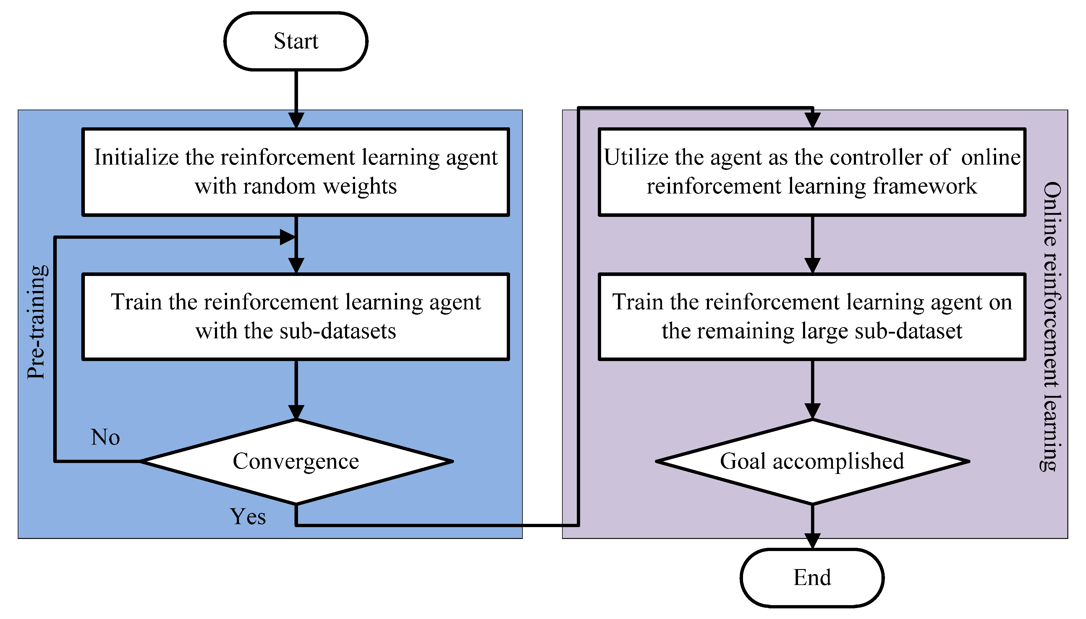
3.4. Online Reinforcement Learning

As illustrated in Figure 4, the flowchart of the proposed online reinforcement learning mechanism is primarily based on the actor-critic network, policy assessment architecture, maximum entropy, and online modification framework. Under the premise of achieving higher rewards, the actor provides the knowledge to fit the policy, which guides the actions to be taken. The critic’s function is to evaluate the proposed actions. The weights and biases of the actor and critic are iteratively updated until the terminal condition—the acquisition of the optimal policy—is satisfied. The policy and entropy mechanisms are utilized to enhance the agent’s exploration, enabling it to achieve a more universal model.

(a) Objective function: The theoretical formula is established as shown below:

$$J(\pi )={\displaystyle \sum _{t=0}^T}{E}_{(s_t,a_t)~d_{\pi }}[r(s_t,a_t)+\alpha H(\pi (|s_t))]$$

(28)

As can be seen from Equation (26), the objective function consists of a reward term and an entropy term, aiming to maximize the return:

$$H(\pi (•|s_t))=E_{a_t}[-\mathit{log}\pi (a_t|s_t)]$$

(29)

(b) Critic network: By evaluating the implemented actions, the critic network is designed to approximate the soft Q-function, as follows:

$$Q_{soft}(s_t,a_t)\triangleq r(s_t,a_t)+\gamma E_{s_{t+1}~p}[E_{a_t~\pi }[Q_{soft}(s_t,a_t)-\alpha \mathit{log}\pi (a_t|s_t)]]$$

(30)

The soft Q-function is modeled using deep neural networks (DNNs), whose weights are updated based on the soft Bellman residual.

$$J_Q(w)=E_{(s_t,a_t)~D}[{\displaystyle \frac{1}{2}}(Q_{soft}(s_t,a_t)-{\stackrel{\wedge }{Q}}_{soft}(s_t,a_t){)}^2]$$

(31)

where $Q_{soft}(s_t,a_t)$ is the evaluated soft Q-function, and ${\stackrel{\wedge }{Q}}_{soft}(s_t,a_t)$ denotes the target soft Q-function. The parameters of the soft Q-function are updated as shown in Equations (32)–(34).

$$\stackrel{̑}{w}=(1-\tau )\stackrel{̑}{w}+\tau w$$

(32)

$$\begin{array}{l}{\stackrel{̑}{▽}}_w{J}_Q(w)={▽}_w{Q}_{soft}(s_t,a_t)(Q_{soft}(s_t,a_t)-\\ r(s_t,a_t)-\gamma (Q_{soft}(s_{t+1},a_{t+1})-\alpha \mathit{log}{\pi }_{\varphi }(s_{t+1},a_{t+1})))\end{array}$$

(33)

$$w=w-{\lambda }_w{\stackrel{̑}{▽}}_w{J}_Q(w)$$

(34)

(c) Actor network: The actor network enables the integration of policy estimation to search for optimal actions by minimizing the Kullback-Leibler divergence.

$${\pi }_{new}=\underset{\pi \in \Pi }{argmin}{D}_{KL}({\pi }_{old}(|s_t)||{\displaystyle \frac{\mathit{exp}(Q^{{\pi }_{old}}(s_t,))}{Z^{{\pi }_{old}}(s_t)}})$$

(35)

where $\Pi$ denotes a set of policies, and $D_{KL}$ represents the value of the KL divergence, which measures the discrepancy between multiple distributions.

4. Results

4.1. Experiment Data

To evaluate the generalization capability of the proposed estimation model, real-time monitoring data from two alkaline electrolyzers at a hydrogen production plant in Hebei Province, China, were analyzed. Two categories of data, reflecting the inherent trends during the corresponding season, were used to generate the essential set of unmeasured variables. It should be noted that, in the proposed topology, steady-state statistics—including rated power and rated voltage, which play a vital role in assessing the estimation performance—are listed in Figure 5. This figure also illustrates the requisite parameters, such as rated power, rated pressure, rated hydrogen production rate, number of cells, cell area, and operating temperature. The data have a time resolution of 5 min, and the collection period spans from 00:00:16 on 1 July 2023 to 23:59:00 on 31 July 2023, resulting in a total of 8929 data points. As discussed in Section 2.1, Section 2.2 and Section 2.3, the aforementioned parameters significantly influence the inherent trends of the unmeasured variables. In summary, the measured data utilized in this study are listed in

Table 3. The measured parameters for the AEL system.

AEL Model	Measured Parameters
Electrochemical model	$U_{cell,t}$, $I_{cell,t}$, $T$, $P$
Heat transfer model	$T_{s,in,t}$, $T_{s,out,t}$, $T_{a,t}$, $T_{sep,in,t}$, $T_{sep,out,t}$, $T_{c,in,t}$, $T_{c,out,t}$
Mass transfer model	$I_{cell}$, $HTO$, T, $P$

.

4.2. Performance Metrics

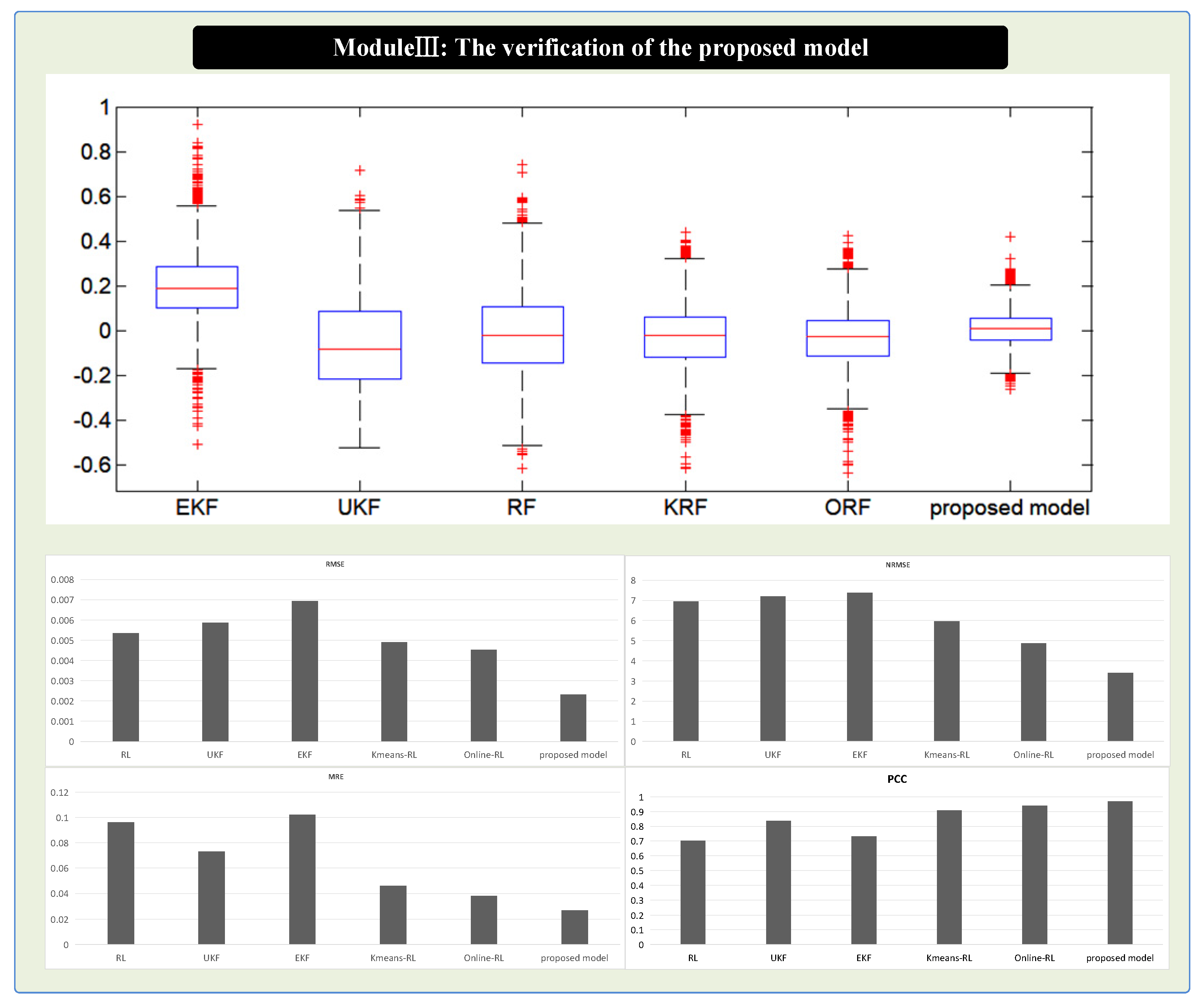
To evaluate the estimation accuracy of the unmeasured variables, four mainstream performance criteria—Mean Relative Error (MRE), Root Mean Square Error (RMSE), Normalized Root Mean Square Error (NRMSE), and Pearson Correlation Coefficient (PCC)—are employed. These metrics are used to assess the extent of improvement achieved by the proposed scheme compared to benchmark models.

$$MRE={\displaystyle \frac{\frac{{\sum }_{i=1}^N(\left|x(t)-\widehat{x}(t)\right|)}{x_r}}{N}}$$

(36)

$$RMSE=\sqrt{{\displaystyle \frac{{\sum }_{i=1}^N[x(t)-\widehat{x}(t){]}^2}{N}}}$$

(37)

$$NRMSE={\displaystyle \frac{RMSE}{\mathit{max}x(t)-\mathit{min}x(t)}}$$

(38)

$$PCC={\displaystyle \frac{{\sum }_{i=1}^N(x(t)-\overline{x}(t))(\stackrel{̑}{x}(t)-\overline{\stackrel{̑}{x}}(t))}{\sqrt{({\sum }_{i=1}^N(x(t)-\overline{x}(t){)}^2{\sum }_{i=1}^N((\stackrel{̑}{x}(t)-\overline{\stackrel{̑}{x}}(t){)}^2)}}}$$

(39)

where $x\left(t\right)$ represents the actual collected data, $\widehat{x}\left(t\right)$ denotes the calculated value derived from the estimated parameters, and $\overline{x}(t)$, $\overline{\stackrel{̑}{x}}(t)$ represent the average values of the monitoring and computational data, respectively. Note that for these four metrics, MRE, RMSE, and NRMSE share a similar origin, indicating that higher fitting accuracy corresponds to smaller values of these statistical criteria. On the other hand, PCC, which measures the linear relationship, yields higher values when the data exhibits a stronger linear correlation.

4.3. Case Study

By comparing the Kmeans-ORL model with alternative estimation engines, namely, the extended Kalman filter (EKF) model and the unscented Kalman filter (UKF) model, we evaluate its performance. Additionally, to demonstrate the advantages of each component in the proposed Kmeans-ORL model, the reinforcement learning (RL) module, the online reinforcement learning (ORL) algorithm, and the hybrid model combining Kmeans and reinforcement learning (KRL) have also been implemented.

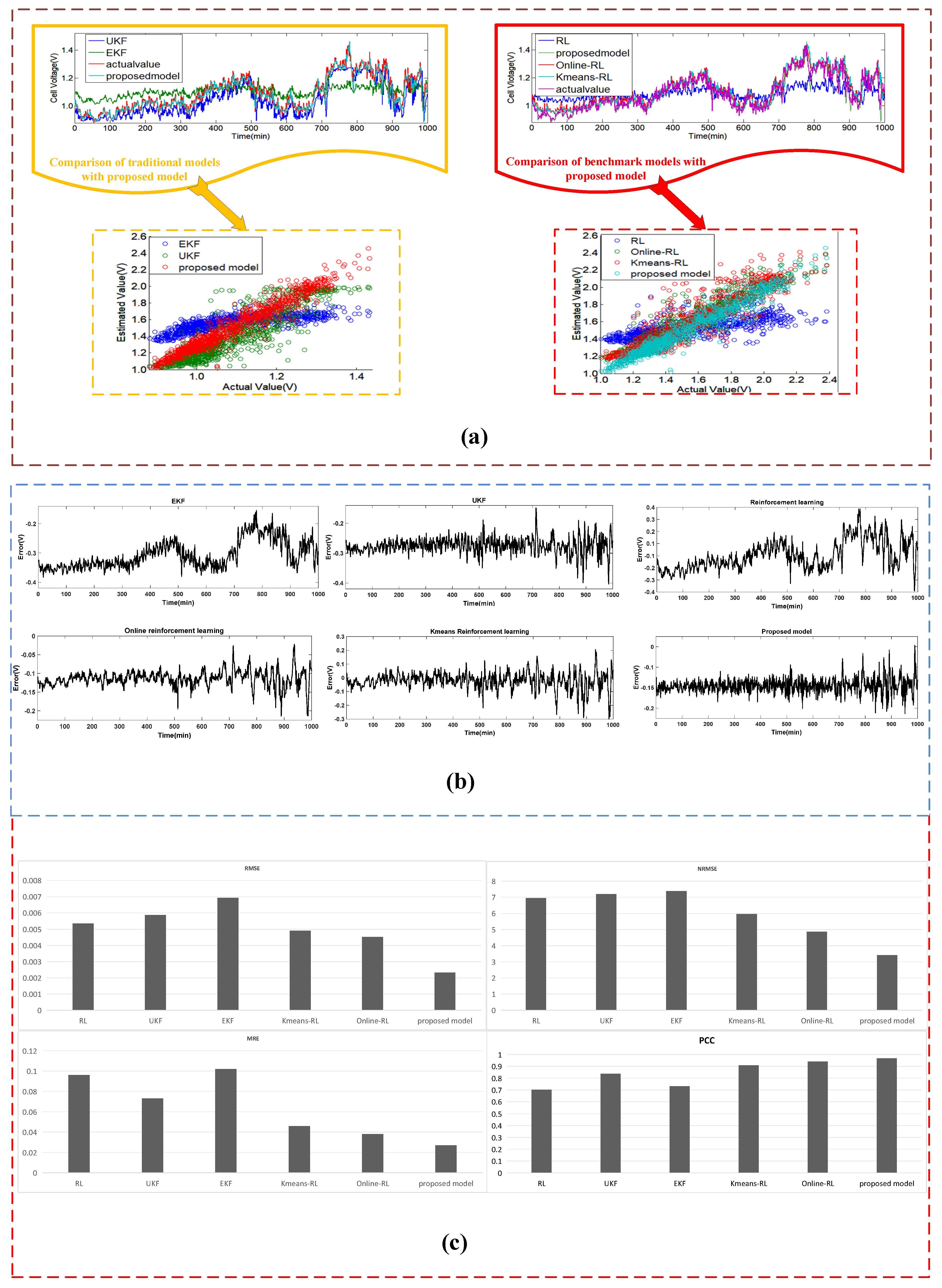
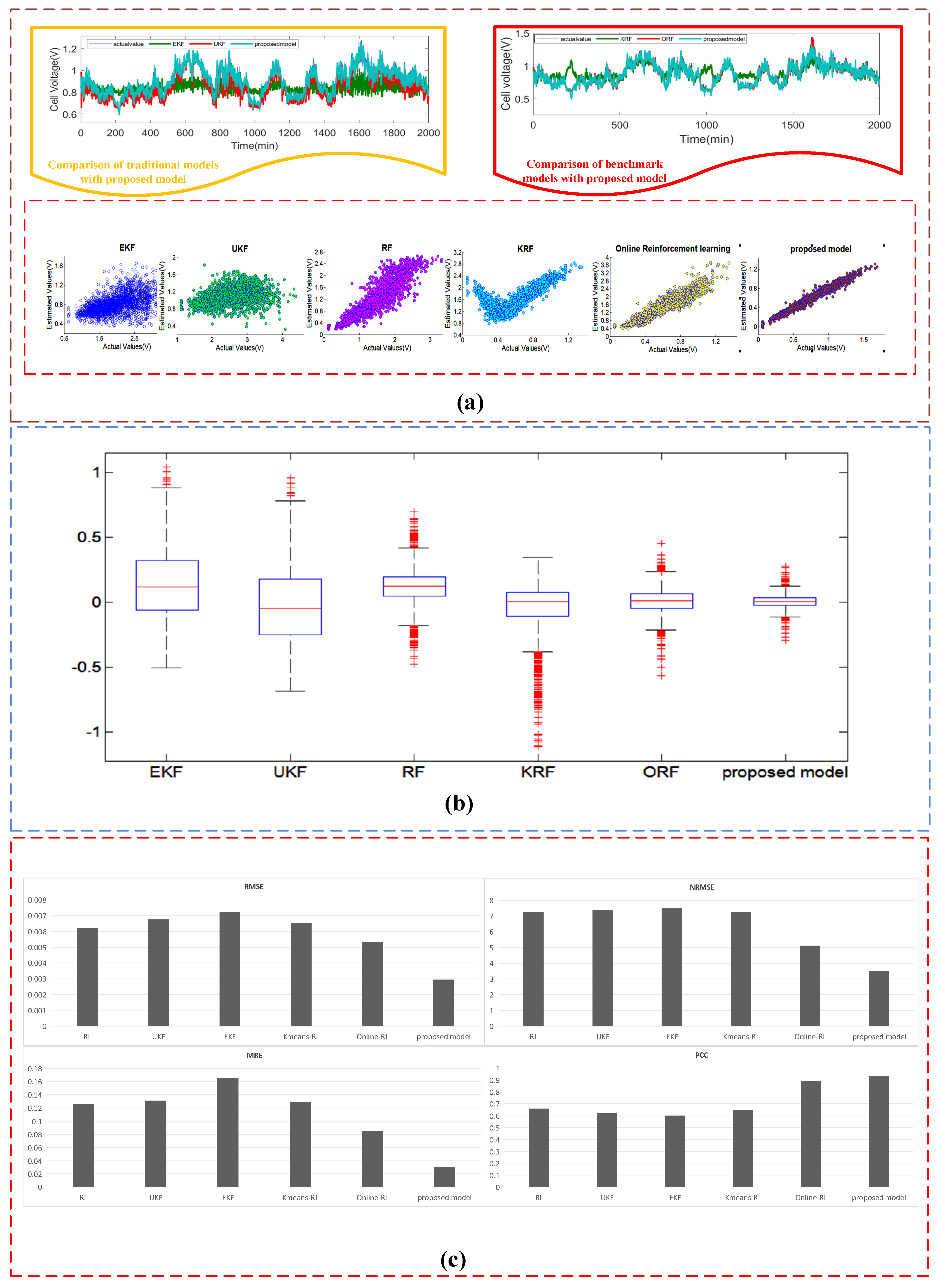
4.3.1. Case I: The Estimated Results of the Dataset #1

The estimated results of the unmeasured variables are listed in

Table 4. Estimated results of the unmeasured variables for Dataset #1.

Sub-System	Parameters	Value	Unit
Electrochemical model	$r_1$	$7.3\times 10^{-5}$	Ω m2
	$r_2$	$4.96\times 10^{-7}$	Ω m2
	$r_3$	$3.36\times 10^{-8}$	Ω m2
	$s$	$8.035\times 10^{-2}$	V
	$t_1$	−0.29	m2/A
	$t_2$	−0.35	m2/A
	$t_3$	0.12	m2/A
Heat transfer model	$C_{sep,lye}$	$4.806\times 10^4$	J/K
	$C_{sep,struc}$	$4.135\times 10^4$	J/K
	$R_{sep}$	$3.56\times 10^{-2}$	K/W
	$C_s$	$1.747\times 10^5$	J/K
	$R$	$3.93\times 10^{-2}$	K/W
	$C_{c,struc}$	$3.955\times 10^5$	J/K
Mass transfer model	$\delta$	610~700	µm
	$S^{H_2}$	0.53~1.24	mol/m3

. Based on the parameter estimation results, the fitting trends of the target variable can be directly observed in Figure 6, Figure 7 and Figure 8.

Table 5. Performance metrics of estimated models for the dataset #1.

Estimating Approaches	Sub System	MRE	RMSE	NRMSE	PCC
EKF	heat transfer	0.087	2.148	19.9	0.536
	electrochemical	0.102	0.00693	7.385	0.731
	mass transfer	0.07102	0.0693	8.385	0.769
UKF	heat transfer	0.092	2.07	19.3	0.813
	electrochemical	0.073	0.00587	7.201	0.837
	mass transfer	0.0673	0.0587	8.201	0.737
RL	heat transfer	0.041	1.492	10.81	0.905
	electrochemical	0.096	0.005353	6.958	0.702
	mass transfer	0.0596	0.0485	7.958	0.802
ORL	heat transfer	0.028	0.748	6.9	0.953
	electrochemical	0.038	0.004521	4.865	0.94
	mass transfer	0.038	0.0345	5.865	0.931
KRL	heat transfer	0.039	0.768	7.15	0.945
	electrochemical	0.046	0.00491	5.958	0.909
	mass transfer	0.046	0.03491	6.958	0.929
Proposed model	heat transfer	0.025	0.635	5.9	0.963
	electrochemical	0.027	0.00232	3.41	0.968
	mass transfer	0.027	0.0232	4.41	0.952

highlights the best-fitting performance in bold font, demonstrating the superior accuracy of the proposed model compared to the benchmark models. This is evident across the three sub-components of the AEL system in the first experiment. Notably, the estimated results for the mass transfer models differ from the others. While the other models exhibit small-scale fluctuations, leading to the use of mean values, the mass transfer models show fluctuations within a specific range. Therefore, the estimated results for these two parameters are presented as a range.

To further demonstrate the superiority of the core components within the proposed Kmeans-online reinforcement learning model, a comparative analysis is presented in Figure 6, Figure 7 and Figure 8 and Table 5. The intuitive conclusions, derived from the comparison between the proposed model and benchmark approaches using various combined schemes, are elaborated as follows:

(1) For verification I, the preponderance that the reinforcement learning model surpasses the existing methods which are adopted in other research endeavors has been vividly illustrated. As can be clearly seen from the figures and metrics, the erratic fitting results are revealed from the EKF and UKF strategies in the electrochemical, heat transfer, and mass transfer sub-systems. Specifically, for the electrochemical sub-system, in terms of the RMSE, MRE, and NRMSE criteria, the RL model generates the lowest values of 0.005353, 0.096, and 7.201, which have dwindled by 0.001577, 0.006, and 0.427 compared to the EKF strategy. With respect to the promotion when compared with the UKF approach, the RL scheme produces reductions in the three relevant metrics by 0.000517, −0.023, and 0.243. The greater value of the PCC index indicates the presence of more linearized characteristics. By means of the depicted trend and statistical results from Figure 6, Figure 7 and Figure 8 and Table 4, RL achieves the best value, which is 0.702, compared to the two traditional models. As for the heat transfer sub-system, a similar phenomenon was illustrated. By assessing the RMSE, MRE, and NRMSE indices, the RL model lowers the values by 0.656, 0.046, and 9.09 compared to the EKF algorithm. Regarding the enhancement when compared with the UKF approach, the RL module reduces the three corresponding metrics by 0.578, 0.051, and 8.49 and increases the PCC by 0.092. With the aim of judging the estimated outcomes in the mass transfer sub-system, the identical performance evaluation is implemented, which further reveals the merits of the RL mechanism.

(2) To evaluate the additional optimized aspects of the Kmeans and online learning schemes, the composite models, including the Kmeans reinforcement learning module and online reinforcement learning platform, are regarded as benchmark technologies to evaluate the preceding estimated capabilities of the reinforcement learning model. For Dataset #1, the Kmeans reinforcement learning model facilitates the reduction of RMSE, MRE, and NRMSE relative to the reinforcement learning model by 0.000443, 0.005, and 1, respectively, in the electrochemical sub-system. As for the heat transfer sub-system, the corresponding improvements are 0.724, 0.002, and 3.66, respectively. Even for the mass transfer system, the Kmeans reinforcement learning model also obtains prominent reductions of 0.01359, 0.0136, and 1 when inferring the dynamic fluctuation of unmeasured parameters. As illustrated within the calculated criteria, the online reinforcement learning platform exhibits similar behaviors with the above-mentioned process. The RMSE, MRE, and NRMSE of the online reinforcement learning platform reach 0.004521, 0.038, and 4.865 for the electrochemical system, which represent reductions of approximately 0.00832, 0.058, and 1.0003, respectively. The corresponding values for evaluating the heat transfer system are 0.748, 0.028, and 6.9. In the scenario of estimating the mass transfer, the targeted values are 0.0345, 0.038, and 5.865, which result in positive enhancements compared to the reinforcement learning model to a certain degree. Regarding the PCC index, the three compared models also provide refined results, in which the Kmeans reinforcement learning methodology achieves increases of 0.04, 0.207, and 0.127, and the online reinforcement learning platform achieves increases of 0.048, 0.238, and 0.002, which can be directly observed in Figure 6, Figure 7 and Figure 8 and Table 4. It should be noted that, owing to the computed criteria, the Kmeans clustering model and online learning scheme strengthen the significant impacts on the estimated tasks.

(3) To further provide a more stable and efficient estimator which can overcome the drawbacks induced by the inherently complex running environment within the AEL system, Kmeans clustering analysis and the online learning mechanism are embedded into the reinforcement learning model simultaneously to provide a better solution. With the strong proof given by the experimental results, comprehensive superiority can be obtained by the proposed model. In accordance with the previous demonstration, the Kmeans clustering analysis and online reinforcement learning are adopted to address the argument arising from the obscure spatial features by conducting a comparison with the proposed model, illustrating the determining role in the proposed model. We can intuitively discover that the proposed model enhances these four indices by 0.00259, 0.019, 2.548, and 0.059 in the field of assessing the electrochemical model when compared with the Kmeans reinforcement learning. This phenomenon also exists in the comparison for the heat transfer and mass transfer systems. As for the online reinforcement learning model, the proposed model achieves improvements of approximately 0.001021, 0.017, 1.455, and 0.028 in the electrochemical model; 0.0113, 0.011, 1.455, and 0.021 in the mass transfer system; and 0.113, 0.003, 1, and 0.01 in the heat transfer model, which means that the contribution of core components can be fully explored in terms of the estimation accuracy.

Figure 6. The performance of the estimated results of the electrochemical model for the dataset #1: (a) Scatter Diagram of Actual Values and Estimated Values; (b) Error Series of Benchmark Models; (c) Metrics of Benchmark Models.

Figure 6. The performance of the estimated results of the electrochemical model for the dataset #1: (a) Scatter Diagram of Actual Values and Estimated Values; (b) Error Series of Benchmark Models; (c) Metrics of Benchmark Models.

Figure 7. The performance of the estimated results of the heat transfer model for the dataset #1: (a) Scatter Diagram of Actual Values and Estimated Values; (b) Error Series of Benchmark Models; (c) Metrics of Benchmark Models.

Figure 7. The performance of the estimated results of the heat transfer model for the dataset #1: (a) Scatter Diagram of Actual Values and Estimated Values; (b) Error Series of Benchmark Models; (c) Metrics of Benchmark Models.

Figure 8. The performance of the estimated results of the mass transfer model for the dataset #1: (a) Scatter Diagram of Actual Values and Estimated Values; (b) Error Series of Benchmark Models; (c) Metrics of Benchmark Models.

Figure 8. The performance of the estimated results of the mass transfer model for the dataset #1: (a) Scatter Diagram of Actual Values and Estimated Values; (b) Error Series of Benchmark Models; (c) Metrics of Benchmark Models.

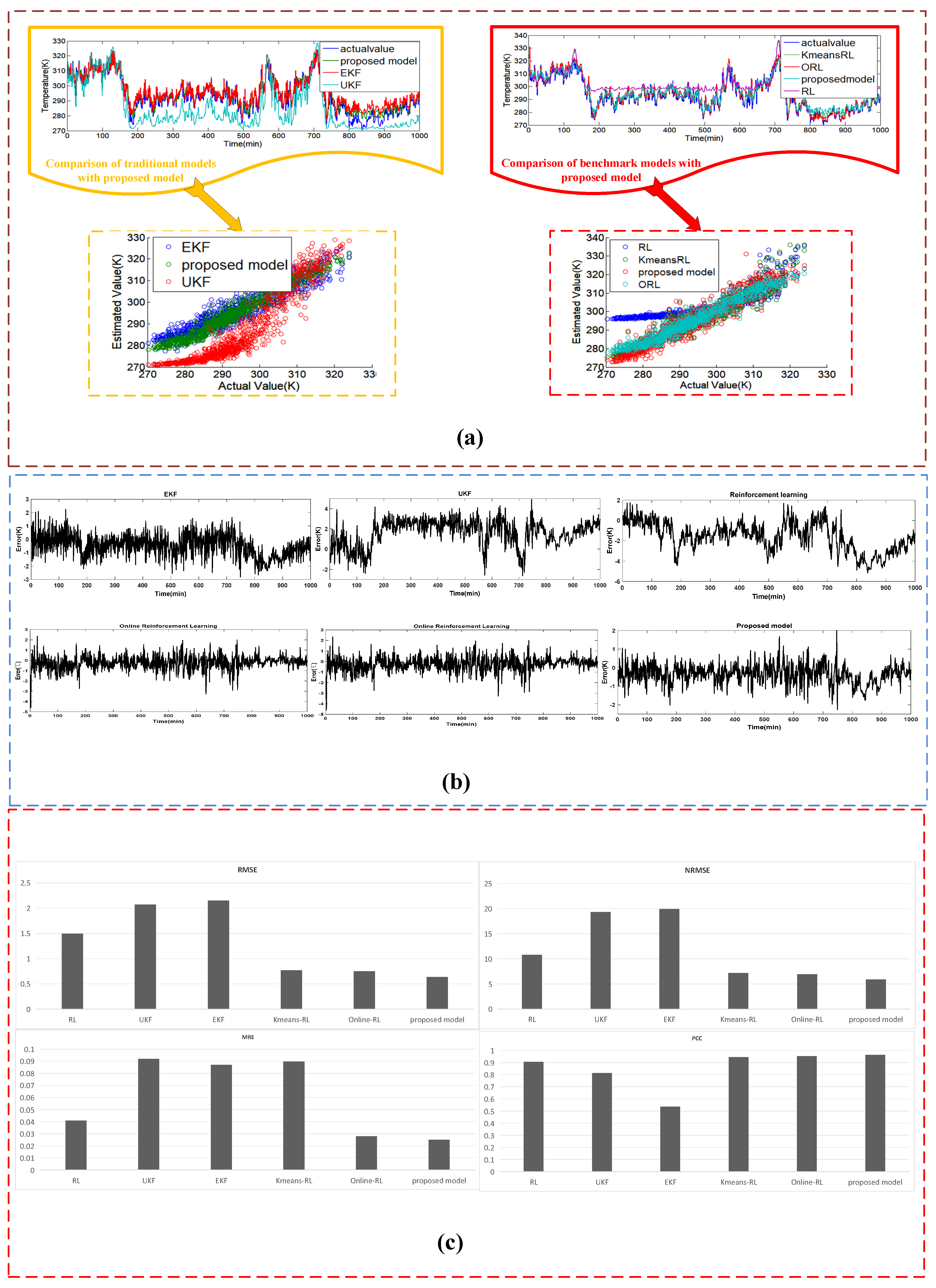
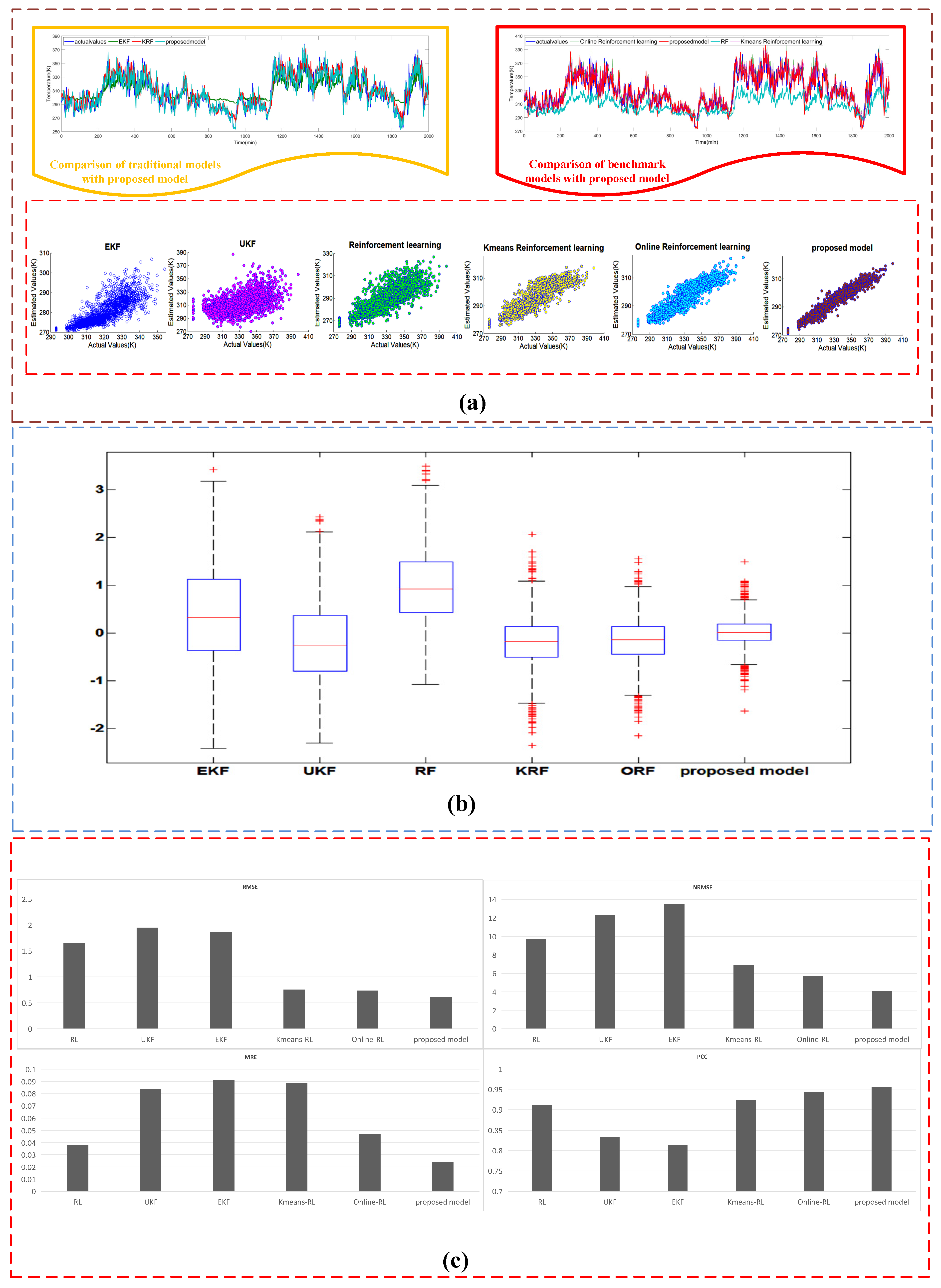
4.3.2. Case II: The Estimated Results of the Dataset #2

Case II evaluates the candidate proposed module by handling this specific dataset. Regarding the estimated performance, the estimators, including all the benchmark models, produce experimental results similar to those mentioned in Case I. However, significant conclusions can still be intuitively drawn, as displayed in Figure 9, Figure 10 and Figure 11 and

Table 6. Estimated results of the unmeasured variables for the dataset #2.

Sub-System	Parameters	Value	Unit
Electrochemical model	$r_1$	$7.12\times 10^{-5}$	Ω m2
	$r_2$	$4.45\times 10^{-7}$	Ω m2
	$r_3$	$4.75\times 10^{-8}$	Ω m2
	$s$	$8.758\times 10^{-2}$	V
	$t_1$	−0.51	m2/A
	$t_2$	−0.65	m2/A
	$t_3$	0.02	m2/A
Heat transfer model	$C_{sep,lye}$	$4.202\times 10^4$	J/K
	$C_{sep,struc}$	$3.569\times 10^4$	J/K
	$R_{sep}$	$3.88\times 10^{-2}$	K/W
	$C_s$	$1.622\times 10^5$	J/K
	$R$	$3.123\times 10^{-2}$	K/W
	$C_{c,struc}$	$3.452\times 10^5$	J/K
Mass transfer model	$\delta$	600~690	µm
	$S^{H_2}$	0.42~1.15	mol/m3

and

Table 7. Performance metrics of estimated models for the dataset #2.

Estimating Approaches	Sub system	MRE	RMSE	NRMSE	PCC
EKF	heat transfer	0.091	1.86	13.5	0.813
	electrochemical	0.165	0.00721	7.498	0.601
	mass transfer	0.07255	0.0688	8.972	0.716
UKF	heat transfer	0.084	1.95	12.3	0.834
	electrochemical	0.131	0.006765	7.391	0.624
	mass transfer	0.0685	0.0597	8.731	0.754
RL	heat transfer	0.038	1.651	9.73	0.912
	electrochemical	0.126	0.006238	7.265	0.659
	mass transfer	0.06346	0.0512	8.234	0.834
ORL	heat transfer	0.047	0.735	5.73	0.943
	electrochemical	0.085	0.00532	5.112	0.89
	mass transfer	0.049	0.0445	6.345	0.912
KRL	heat transfer	0.08865	0.7548	6.86	0.923
	electrochemical	0.129	0.00655	7.288	0.643
	mass transfer	0.052	0.0437	6.774	0.898
Proposed model	heat transfer	0.024	0.612	4.09	0.956
	electrochemical	0.03	0.00295	3.51	0.932
	mass transfer	0.033	0.0384	5.47	0.926

.

(1) To further evaluate the merits of the reinforcement learning algorithm, the calculated criteria, through which the superiority and accuracy can be demonstrated, are also analyzed. The corresponding values of RMSE, MRE, NRMSE, and PCC metrics describing the electrochemical system are 0.006238, 0.126, 7.265%, and 0.659, respectively, for the reinforcement learning model. Meanwhile, in the heat transfer sub-system, the RMSE, MRE, NRMSE, and PCC are 1.651, 0.038, 9.73%, and 0.912, respectively. A similar phenomenon appears in the task of assessing the mass transfer sub-system, where the relevant criteria are 0.0512, 0.06346, 8.234%, and 0.834. In contrast, the EKF model ranks last in estimating this dataset, producing 0.00721, 0.165, 7.498%, and 0.601 for the electrochemical system in terms of the four indices, respectively. As for the other two sub-systems, the EKF model produces the closest results. The corresponding values of RMSE, MRE, NRMSE, and PCC increase by approximately 20% compared to the reinforcement learning model.

(2) In this case, the advantages of the Kmeans clustering analysis, online learning, and reinforcement learning mechanism still exist in most cases. For the electrochemical system, among the mentioned models, the ranking of EKF, UKF, RL, Kmeans reinforcement learning, online reinforcement learning, and the proposed approaches in terms of accuracy, from best to worst, is EKF, UKF, RL, Kmeans reinforcement learning, online reinforcement learning, and the proposed approach, with the RMSE values of 0.00721, 0.006765, 0.00655, 0.006238, 0.00532, and 0.00295, respectively. The corresponding values in terms of the MRE index are 0.165, 0.131, 0.129, 0.126, 0.085, and 0.03. However, the rank changes to EKF, UKF, Kmeans reinforcement learning, reinforcement learning, online reinforcement learning, and proposed model. From these criteria and relevant curve graphs, error boxplots, and histograms, it can be easily found that the Kmeans reinforcement learning shows some degradation compared to reinforcement learning due to the inappropriate K value, which we will further optimize in future research. As for the other two metrics, certain improvements are achieved due to the optimized components. For instance, the proposed model improves by 76.7%, 54.96%, 51.84%, and 31% for MRE, RMSE, NRMSE, and PCC metrics in the context of the electrochemical system compared with Kmeans reinforcement learning. The corresponding values for the heat transfer model are 72.93%, 18.92%, 40.38%, and 3.45%, and the values for the mass transfer model are 36.54%, 12.13%, 19.25%, and 3.02%. By comparing the proposed model to the online reinforcement learning model, the enhancements of the proposed model are distributed as 64.71%, 44.55%, 31.44%, and 4.51% for the electrochemical subsystem. The relevant values for the heat transfer subsystem are 48.94%, 16.73%, 28.62%, and 1.36%. As for the mass transfer subsystem, the improvements reach 32.65%, 13.71%, 13.79%, and 1.51%. These similar trends emerge in the evaluation of the improvements achieved by the Kmeans reinforcement learning and online reinforcement learning compared to the reinforcement learning scheme, which is clearly illustrated in the graphs. In these mentioned figures, the boxplots represent the error performance of the estimated results by implicitly describing the maximum, mean, and minimum values of the error series, which are calculated from the comparative models, including the EKF, UKF, RF, KRF, ORF, and proposed model.

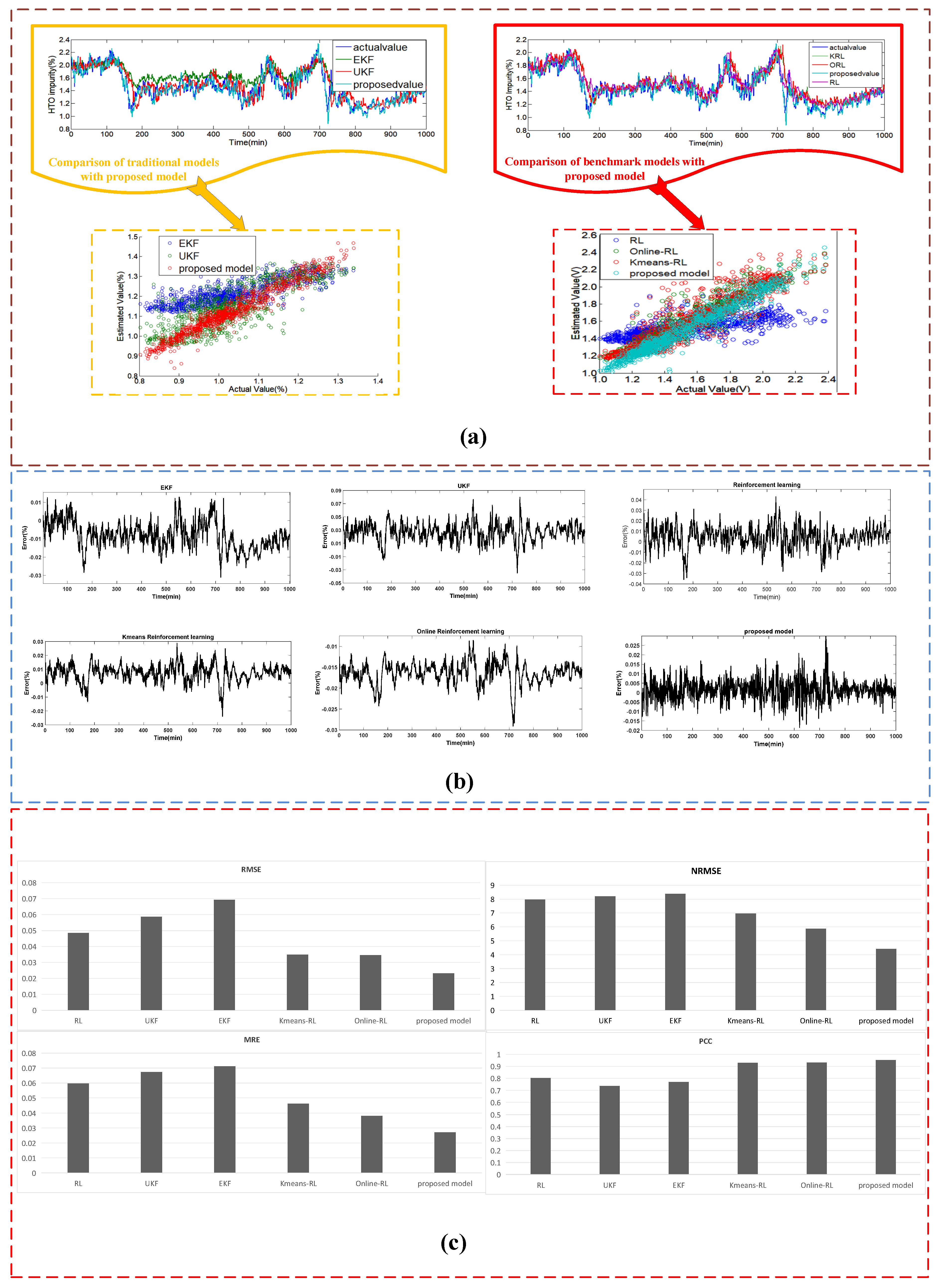
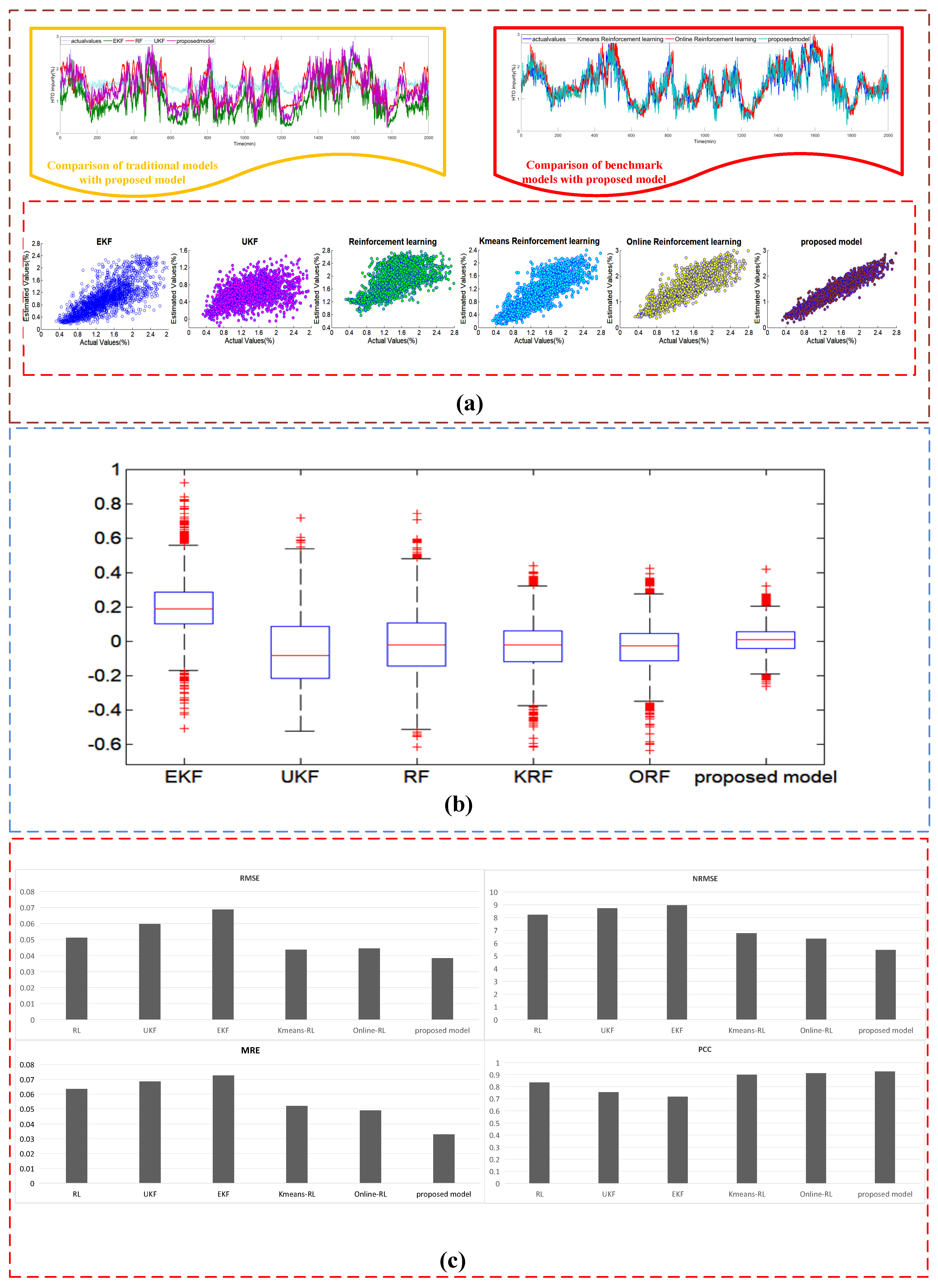
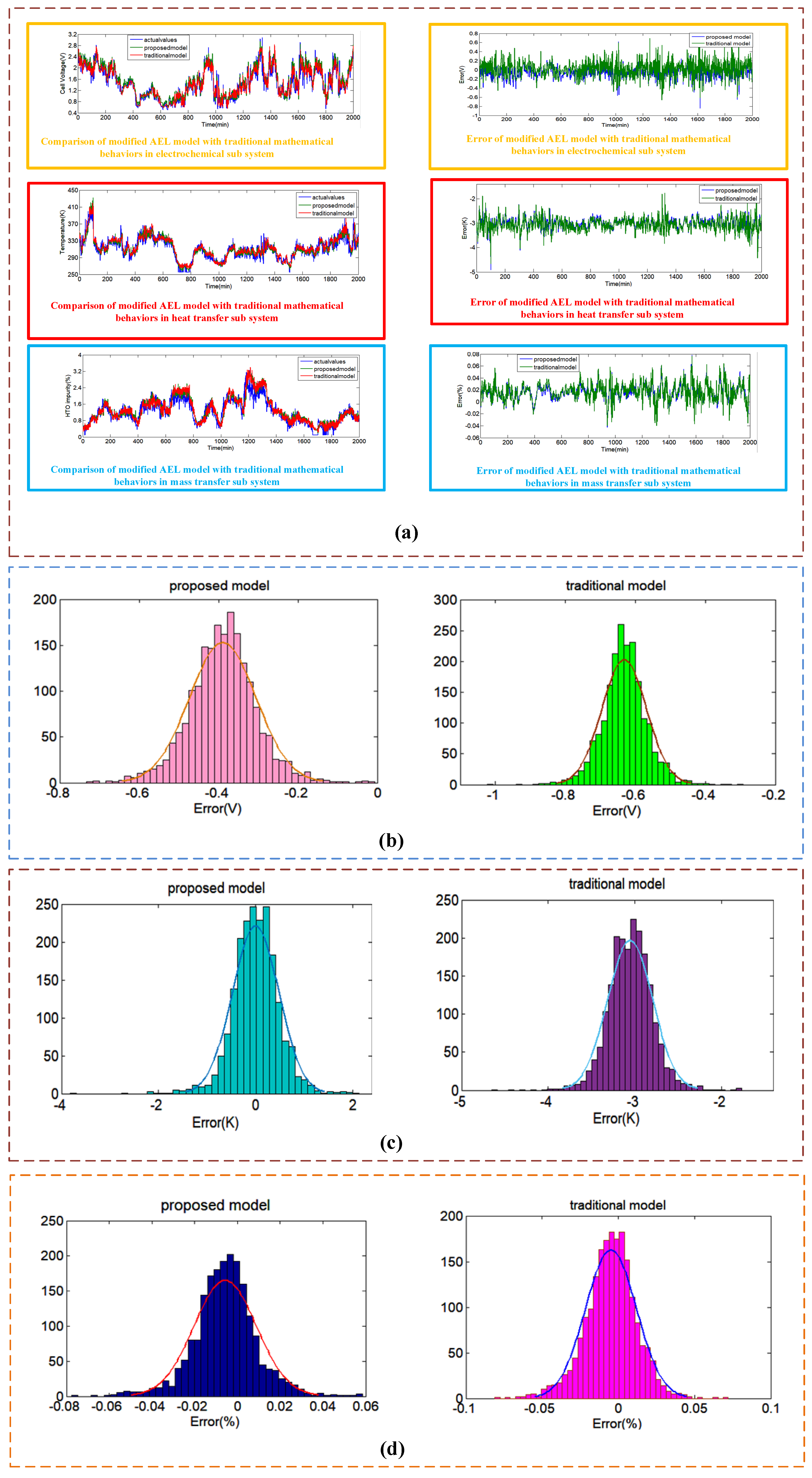
4.3.3. Case III Comparison with the Modified AEL Systems for Dataset #3

With the aim of presenting the superior performance achieved by the modified AEL system that embeds the momentum factor into its mathematical theories, as can be seen from Equations (2), (8) and (11), Dataset #3 and the proposed estimation model were adopted to conduct the verification experiment, the results of which are listed in

Table 8. Estimated results of the unmeasured variables for the dataset #3.

Sub-System	Parameters	Value	Unit
Electrochemical model	$r_1$	$6.95\times 10^{-5}$	Ω m2
	$r_2$	$4.31\times 10^{-7}$	Ω m2
	$r_3$	$4.98\times 10^{-8}$	Ω m2
	$s$	$7.433\times 10^{-2}$	V
	$t_1$	−0.62	m2/A
	$t_2$	−0.60	m2/A
	$t_3$	0.11	m2/A
Heat transfer model	$C_{sep,lye}$	$4.315\times 10^4$	J/K
	$C_{sep,struc}$	$3.522\times 10^4$	J/K
	$R_{sep}$	$3.97\times 10^{-2}$	K/W
	$C_s$	$1.438\times 10^5$	J/K
	$R$	$3.056\times 10^{-2}$	K/W
	$C_{c,struc}$	$3.568\times 10^5$	J/K
Mass transfer model	$\delta$	620~700	µm
	$S^{H_2}$	0.38~1.03	mol/m3

and

Table 9. Performance metrics of estimated models for the dataset #3.

Estimating Approaches	Sub System	MRE	RMSE	NRMSE	PCC
Traditional AEL system	heat transfer	0.042	0.724	5.36	0.922
	electrochemical	0.081	0.00632	5.768	0.854
	mass transfer	0.041	0.0398	6.553	0.865
Proposed AEL system	heat transfer	0.039	0.685	4.75	0.933
	electrochemical	0.075	0.00611	5.431	0.875
	mass transfer	0.032	0.0348	6.12	0.911

and Figure 12.

(1) As can be seen from Table 8 and Table 9 and Figure 12, the proposed model presented more accurate and efficient estimation results in handling the modified AEL system compared to the traditional AEL system. For the electrochemical sub-system, the values of the RMSE, MRE, NRMSE, and PCC metrics for the modified AEL system were 0.00611, 0.075, 5.431, and 0.854. In terms of the traditional AEL sub-system, the values of the four relevant criteria were 0.00632, 0.081, 5.768, and 0.875. Meanwhile, in the heat transfer sub-system, the RMSE, MRE, NRMSE, and PCC of the modified AEL system were 0.685, 0.039, 4.75, and 0.933. In contrast, the traditional AEL system yielded values of 0.724, 0.042, 5.36, and 0.922 for the corresponding metrics. As for the remaining mass transfer system, a similar phenomenon has also emerged, which comprehensively verifies the superiority of the theoretical modification upgrade.

(2) From the observations depicted in Figure 12, the comparative line diagrams of actual values and estimated variables presented similar fluctuating trends in the three sub-systems. The proposed model generated lines closer to the actual values compared to the traditional model. The same situation can be intuitively seen in the error series, in which the lines of the traditional model encompassed the proposed model in most cases. Moreover, from the histograms of the error series of the three sub-systems, the bandwidth of the proposed model was narrower compared to the traditional model, and the corresponding errors had smaller values.

5. Conclusions

This paper proposes a dynamic parameter estimation model that synthesizes modified mathematical theories, clustering analysis, online learning, and reinforcement learning. Benefiting from the proposed model, key knowledge within the AEL system can be fully explored under the predefined modified mechanism. The superiority of the proposed model can be attributed to three factors:

(1) By implanting the momentum factor into the mathematical theory, which bridges the gap between the historical data and unmeasured variables to achieve higher accuracy and convergence.

(2) K-means clustering analysis divides the isolated dataset into several categories, thereby eliminating the significant obstacles posed by the complex and nonlinear relationships among the measured variables. Subsequently, the associated online reinforcement learning scheme can enhance the reliability and stability of the system.

(3) This approach proposes a reinforcement learning strategy that leverages the advantages of online learning to estimate the parameters of an Alkaline Electrolysis (AEL) system. This method addresses the challenges posed by the strong nonlinearity of the system’s dynamic behavior and the correlations among parameters. Experimental validation on the AEL system confirmed the accuracy and robustness of the proposed approach. Compared to existing parameter estimation methods such as EKF and UKF, the proposed method achieved improvements of 76.7%, 54.96%, 51.84%, and 31% in terms of RMSE, NRMSE, PCC, and MPE, respectively. Additionally, the proposed method provides valuable physical insights into the dynamics of the AEL system.

References

1. Xu, Y.; Lv, H.; Lu, H.; Quan, Q.; Li, W.; Cui, X.; Liu, G.; Jiang, L. Mg/seawater batteries driven self-powered direct seawater electrolysis systems for hydrogen production. Nano Energy 2022, 98, 107295. [Google Scholar] [CrossRef]
2. Qiu, X.; Zhang, H.; Qiu, Y.; Zhou, Y.; Zang, T.; Zhou, B.; Qi, R.; Lin, J.; Wang, J. Dynamic parameter estimation of the alkaline electrolysis system combining Bayesian inference and adaptive polynomial surrogate models. Appl. Energy 2023, 348, 121533. [Google Scholar] [CrossRef]
3. Panah, P.G.; Cui, X.; Bornapour, M.; Hooshmand, R.-A.; Guerrero, J.M. Marketability analysis of green hydrogen production in Denmark: Scale-up effects on grid-connected electrolysis. Int. J. Hydrogen Energy 2022, 47, 12443–12455. [Google Scholar] [CrossRef]
4. Sebbahi, S.; Assila, A.; Belghiti, A.A.; Laasri, S.; Kaya, S.; Hlil, E.K.; Rachidi, S.; Hajjaji, A. A comprehensive review of recent advances in alkaline water electrolysis for hydrogen production. Int. J. Hydrogen Energy 2024, 82, 583–599. [Google Scholar] [CrossRef]
5. de Groot, M.T.; Kraakman, J.; Barros, R.L.G. Optimal operating parameters for advanced alkaline water electrolysis. Int. J. Hydrogen Energy 2022, 47, 34773–34783. [Google Scholar] [CrossRef]
6. Sanchez, M.; Amores, E.; Rodriguez, L.; Clemente-Jul, C. Semi-empirical model and experimental validation for the performance evaluation of a 15 kW alkaline water electrolyzer. Int. J. Hydrogen Energy 2018, 43, 20332–20345. [Google Scholar] [CrossRef]
7. Huang, D.; Xiong, B.; Fang, J.; Hu, K.; Zhong, Z.; Ying, Y.; Ai, X.; Chen, Z. A multiphysics model of the compactly-assembled industrial alkaline water electrolysis cell. Appl. Energy 2022, 314, 118987. [Google Scholar] [CrossRef]
8. Kim, H.; Park, M.; Lee, K.S. One-dimensional dynamic modeling of a high-pressure water electrolysis system for hydrogen production. Int. J. Hydrogen Energy 2013, 38, 2596–2609. [Google Scholar] [CrossRef]
9. Sakas, G.; Ibanez-Rioja, A.; Ruuskanen, V.; Kosonen, A.; Ahola, J.; Bergmann, O. Dynamic energy and mass balance model for an industrial alkaline water electrolyzer plant process. Int. J. Hydrogen Energy 2022, 47, 4328–4345. [Google Scholar] [CrossRef]
10. Zhang, J.; Zhao, X. Digital twin of wind farms via physics-informed deep learning. Energy Convers. Manag. 2023, 293, 117507. [Google Scholar] [CrossRef]
11. Abomazid, A.M.; El-Taweel, N.A.; Farag, H.E. Novel analytical approach for parameters identification of PEM electrolyzer. IEEE Trans. Ind. Inf. 2022, 18, 5870–5881. [Google Scholar]
12. El-Fergany, A.A. Extracting optimal parameters of PEM fuel cells using Salp Swarm Optimizer. Renew. Energy 2018, 119, 641–648. [Google Scholar]
13. Mirjalili, S. SCA: A Sine Cosine Algorithm for solving optimization problems. Knowl. Based Syst. 2016, 96, 120–133. [Google Scholar]
14. Ben Messaoud, R.; Midouni, A.; Hajji, S. PEM fuel cell model parameters extraction based on moth-flame optimization. Chem. Eng. Sci. 2021, 229, 116100. [Google Scholar]
15. Chen, K.; Peng, H.; Zhang, J.; Chen, P.; Ruan, J.; Li, B.; Wang, Y. Optimized Demand-Side Day-Ahead Generation Scheduling Model for a Wind-Photovoltaic-Energy Storage Hydrogen Production System. ACS Omega 2022, 7, 43036–43044. [Google Scholar]
16. Abaza, A.; El-Sehiemy, R.A.; Mahmoud, K.; Lehtonen, M.; Darwish, M.M. Optimal estimation of proton exchange membrane fuel cells parameter based on coyote optimization algorithm. Appl. Sci. 2021, 11, 2052. [Google Scholar] [CrossRef]
17. Gunay, M.E.; Tapan, N.A.; Akkoc, G. Analysis and modeling of high-performance polymer electrolyte membrane electrolyzers by machine learning. Int. J. Hydrogen Energy 2022, 47, 2134–2151. [Google Scholar]
18. Wang, M.; Zhu, H. Machine learning for transition-metal-based hydrogen generation electrocatalysts. ACS Catal. 2021, 11, 3930–3937. [Google Scholar]
19. Jang, D.; Choi, W.; Cho, H.-S.; Cho, W.C.; Kim, C.H.; Kang, S. Numerical modeling and analysis of the temperature effect on the performance of an alkaline water electrolysis system. J. Power Sources 2021, 506, 230106. [Google Scholar]
20. Li, Y.; Zhang, T.; Ma, J.; Deng, X.; Gu, J.; Yang, F.; Ouyang, M. Study the effect of lye flow rate, temperature, system pressure and different current density on energy consumption in catalyst test and 500W commercial alkaline water electrolysis. Mater. Today Phys. 2022, 22, 100606. [Google Scholar]
21. Qiu, Y.; Zhou, B.; Zang, T.; Zhou, Y.; Chen, S.; Qi, R.; Li, J.; Lin, J. Extended load flexibility of utility-scale P2H plants: Optimal production scheduling considering dynamic thermal and HTO impurity effects. Renew. Energy 2023, 217, 119198. [Google Scholar]
22. Kojima, H.; Nagasawa, K.; Todoroki, N.; Ito, Y.; Matsui, T.; Nakajima, R. Influence of renewable energy power fluctuations on water electrolysis for green hydrogen production. Int. J. Hydrogen Energy 2023, 48, 4572–4593. [Google Scholar]
23. Jang, D.; Cho, H.-S.; Kang, S. Numerical modeling and analysis of the effect of pressure on the performance of an alkaline water electrolysis system. Appl. Energy 2021, 287, 116554. [Google Scholar]
24. Rodriguez, J.; Amores, E. CFD modeling and experimental validation of an alkaline water electrolysis cell for hydrogen production. Processes 2020, 8, 1634. [Google Scholar] [CrossRef]
25. Haverkort, J.W.; Rajaei, H. Voltage losses in zero-gap alkaline water electrolysis. J. Power Sources 2021, 497, 229864. [Google Scholar]
26. Hammoudi, M.; Henao, C.; Agbossou, K.; Dubé, Y.; Doumbia, M.L. New multi-physics approach for modelling and design of alkaline electrolyzers. Int. J. Hydrogen Energy 2012, 37, 13895–13913. [Google Scholar]
27. Qi, R.; Gao, X.; Lin, J.; Song, Y.; Wang, J.; Qiu, Y.; Liu, M. Pressure control strategy to extend the loading range of an alkaline electrolysis system. Int. J. Hydrogen Energy 2021, 46, 35997–36011. [Google Scholar]
28. Qi, R.; Li, J.; Lin, J.; Song, Y.; Wang, J.; Cui, Q.; Qiu, Y.; Tang, M.; Wang, J. Thermal modeling and controller design of an alkaline electrolysis system under dynamic operating conditions. Appl. Energy 2023, 332, 120551. [Google Scholar]
29. Xia, Y.H.; Cheng, H.R.; He, H.H.; Hu, Z.Y.; Wei, W. Efficiency Enhancement for Alkaline Water Electrolyzers Directly Driven by Fluctuating PV Power. IEEE Trans. Ind. Electron. 2024, 71, 5755–5765. [Google Scholar]
30. Cantisani, N.; Dovits, J.; Jørgensen, J. Dynamic modeling of an alkaline electrolyzer plant for process simulation and optimization. arXiv 2023, arXiv:2311.09882. [Google Scholar]
Figure 1. The structure of the AEL system.
Processes 13 01009 g001
Figure 2. Architecture of the proposed model.
Processes 13 01009 g002aProcesses 13 01009 g002b
Figure 3. The flowchart of the proposed online reinforcement learning with the pretraining framework.
Processes 13 01009 g003
Figure 4. Flowchart of the online reinforcement learning.
Processes 13 01009 g004
Figure 5. Description of the data sets and the platform of the ALE system. (a) Description of the data sets; (b) the platform of the ALE system.
Processes 13 01009 g005
Figure 9. The performance of the estimated results of the electrochemical model for the dataset #2: (a) Scatter Diagram of Actual Values and Forecasting Values; (b) Boxplot for Error Series of Benchmark Models; (c) Metrics of Benchmark Models.
Processes 13 01009 g009
Figure 10. The performance of the estimated results of the heat transfer model for the dataset #2: (a) Scatter Diagram of Actual Values and Forecasting Values; (b) Boxplot for Error Series of Benchmark Models; (c) Metrics of Benchmark Models.
Processes 13 01009 g010
Figure 11. The performance of the estimated results of the mass transfer model for the dataset #2: (a) Scatter Diagram of Actual Values and Forecasting Values; (b) Boxplot for Error Series of Benchmark Models; (c) Metrics of Benchmark Models.
Processes 13 01009 g011
Figure 12. A comparison of the proposed mathematical models with traditional models on dataset #3: (a) Line Diagram of Actual Values and Estimating Values; (b) Histfit for Error Series of Electrochemical System; (c) Histfit for Error Series of Heat Transfer System; (d) Histfit for Error Series of Mass Transfer System.
Processes 13 01009 g012