Analysis of Safe Mud Density Window for Enhanced Wellbore Stability

Abstract

Deep drilling can lead to the encounter of complex geological conditions, with significant overburden pressure leading to a narrow safety window for mud density. In this study, we deviated wellbore instability conditions using the Mohr–Coulomb and tensile failure criteria, solving for collapse, shear, and fracture pressure using Newton’s method. The safe mud density window is defined between the maximum value of pore and collapse pressures and the minimum value of shear and fracture pressures. The analysis of the Anderson fault stress model, utilizing this method, enables a comprehensive investigation of how the safety mud density window varies with wellbore inclination and azimuth angles under various stress conditions. Additionally, applications in Chinese oilfields illustrate that this methodology can accurately calculate and analyze extremely narrow safety mud density windows at depths ranging from 2000 to 3000 m. In conclusion, this method enables rapid and accurate prediction of mud density limits, improving wellbore stability and reducing drilling risks.

1. Introductions

Ensuring wellbore stability is essential during drilling and extraction processes in oil and gas operations. Wellbore shrinkage can happen when plastic rocks compress into the borehole, while holes may occur due to the caving-in of shale or the disintegration of hard rock. Elevated fluid pressure in the wellbore can unintentionally induce hydraulic fracturing and result in lost circulation, whereas insufficient pressure may lead to the wellbore collapsing. Additionally, high production rates can trigger the influx of solid particles. Such instabilities can lead to challenges like stuck drill pipes and the failure of casing or liners, potentially causing side-tracked holes and abandoned wells. Therefore, maintaining wellbore stability requires carefully balancing uncontrollable factors, such as origin stresses, rock strength, and pore pressure, with controllable drilling mud. Important controllable factors include mud weight, as well as the azimuth angle and inclination of the wellbore [1]. Recent studies have shown that increasing mud and hydrate saturation can significantly enhance wellbore stability in hydrate-bearing sediments, while managing mud temperature and salinity is crucial to prevent borehole collapse [2]. Furthermore, the use of CO₂ fracturing fluids has been demonstrated to effectively facilitate crack propagation in low-permeability reservoirs, highlighting the importance of selecting appropriate drilling fluids to optimize reservoir performance [3].

If the mud weight is higher than necessary, it can invade the formation and cause tensile failure [4]. On the other hand, reducing the mud weight may result in rock collapse failures, referred to as borehole breakouts. As a result, particularly in the inclined sections of the wellbore, it is crucial to keep the drilling mud density within a safe range. This is generally achieved by employing a constitutive model to estimate the stresses surrounding the wellbore, combined with a failure criterion to forecast the ultimate strength of the reservoir rocks. Consequently, a key focus in analyzing wellbore stability is the choice of an appropriate rock strength criterion and the subsequent calculations involved in the assessment.

Coulomb’s criterion [5] for the shear fracture of a brittle material is that total shearing resistance is the sum of cohesive shear strength (independent of direction) and the product of effective normal stress and the coefficient of internal friction (a constant independent of normal stress). The Mohr–Coulomb (M-C) strength criterion [6], describing the relationship between normal stress and shear stress on the failure surface at peak strength, makes it a crucial tool for analyzing rock failure. In offshore drilling operations, where sedimentary rocks are predominant [7], the application of the M-C criterion becomes essential. This is because the unique characteristics of sedimentary rocks necessitate a reliable framework for predicting shear failure and ensuring borehole stability [8]. Therefore, utilizing the M-C criterion is vital for effectively addressing the challenges posed by drilling in sedimentary environments.

Natural oil and gas reservoirs are primarily found in deep, buried-hill-type meta- morphic formations. Thick, organic-rich source rocks, which have reached a high maturity stage, exhibit significant gas generation potential. Furthermore, tectonic evolution has led to the formation of large-scale buried-hill traps [9]. However, the associated over-pressure conditions and tight reservoir characteristics result in a relatively narrow safe mud density window [10,11]. Therefore, the development of natural gas fields demands precise development strategies and effective drilling plan management to maintain drilling fluid within the safe density window under complex conditions, ensuring the protection of the tight reservoir [12].

In this paper, we begin by calculating rock mechanic parameters to determine the stress distribution in deep, inclined drilling, using formation stress as a basis. We identify that the lower limit of the safe mud density window for wellbore stability is determined by the larger value between collapse pressure and pore pressure, while the upper limit is the smaller value between shear pressure and fracture pressure. The pore pressure is calculated using the Eaton method [13]. Collapse pressure and shear pressure are derived from the M-C criterion, and fracture pressure is derived from the tensile failure criterion. We derived the quadratic equation for wellbore pressure based on these guidelines, where the roots of the collapse and shear failure equations represent the collapse pressure and shear pressure, respectively. The larger root of the tensile failure equation corresponds to fracture pressure. We then applied Newton’s method, a stable and efficient algorithm, to solve these equations accurately. Drawing from Anderson’s fault regimes, we created three model groups to assess the effects of azimuth angle (the angle with the maximum horizontal principal stress) and well inclination on the safe mud density window. While this study focuses on the assumption that vertical principal stress is directed vertically downward, we acknowledge that geostress conditions can be complex, and the vertical principal stress may tilt, particularly in the presence of geological features such as folds or faults. This assumption allows for a clearer understanding of the fundamental mechanics involved. Future research could explore the implications of varying principal stress orientations on stress distribution. These analyses form a solid foundation for drilling planning, wellbore design, and mud density optimization. Finally, we apply this methodology to deep subterranean drilling in an oilfield in eastern China, analyzing rock mechanic parameters, optimizing the drilling trajectory, and determining the safe mud density window to ensure safe, efficient, and economical construction.

2. Methodology

In this section, we delve into the analysis of principal stresses, encompassing overburden pressure as well as the minimum and maximum horizontal principal stresses. We also explore pore pressure and the effective stress theory, examining the distribution of stress within vertical wells and then generalizing these findings to the case of inclined wells. Common parameter symbols are presented in the Nomenclature in the back matter, with any specialized parameters being thoroughly explained in their respective subsections.

2.1. Calculation of Rock Mechanics Parameters

Rock mechanic properties are primarily categorized into two key groups: elastic properties and strength properties. Elastic properties encompass Young’s modulus, Poisson’s ratio, bulk modulus, and shear modulus, which quantify the rock’s deformability under stress. Strength properties include compressive strength, tensile strength, cohesion stress, and the internal friction coefficient, reflecting the rock’s capacity to withstand failure. The determination of these properties is achieved through experimental and computational methods. Computational methods, which leverage logging and seismic data, offer the advantage of generating continuous parameter profiles and substantial data volumes for specific well sections or broader study areas. This approach has become prevalent due to its practicality and efficiency [14]. Utilizing these basic parameters allows for the calculation of critical formation pressures, such as pore pressure, fracture pressure, and collapse pressure. These pressures are essential for ascertaining the in situ stress of the wellbore, evaluating the stability of wellbore walls, and confirming the safety of the mud density window.

2.1.1. Analysis of Principal Stresses

It is generally considered that the stress state at the wellbore site is composed of three mutually orthogonal principal stresses: the overburden pressure (vertical principal stress), the minimum horizontal principal stress, and the maximum horizontal principal stress.

2.1.2. Overburden Pressure

The magnitude of ${\sigma }_v$ corresponds to the integration of rock densities from the surface down to the specified depth, $z$. Therefore, the overburden pressure can be written as follows [15]:

$${\sigma }_{\mathrm{v}}={\int }_0^z\rho \left(z\right)g\mathrm{d}z\approx \overline{\rho }gz,$$

(1)

where $\rho \left(z\right)$ is the density as a function of depth, $g$ is gravitational acceleration, and $\overline{\rho }$ is the mean overburden density. In offshore areas, Equation (1) can be corrected for water depth as follows:

$${\sigma }_{\mathrm{v}}\approx {\rho }_{W}g{z}_w+\overline{\rho }g\left(z-z_W\right)$$

(2)

where $z_W$ is the water depth and ${\rho }_W$ is the density of water.

2.1.3. Pore Pressure

From a macroscopic perspective, strata are mainly composed of two parts: sediments and pores, which are typically filled with fluids such as oil, gas, and water. The pressure exerted by these fluids on the surrounding rock is referred to as the pore pressure of the strata. Scholars, both domestically and internationally, have proposed various methods for obtaining pore pressure, including geological analysis [16], seismic methods [17], and well-logging techniques [18]. Among these, methods based on well logging and seismic data can provide relatively reliable pore pressure profiles, with the Eaton method being one commonly used approach. In 1975, Eaton proposed an empirical formula for estimating strata pore pressure based on extensive experimental data from the Gulf of Mexico:

$$P_P={\sigma }_v-\left({\sigma }_v-P_h\right){\left({\displaystyle \frac{∆t_n}{∆t_d}}\right)}^e$$

(3)

where $P_h$ is the formation of hydro-static pressure, $e$ is the compaction coefficient, $∆t_n$ is the measured acoustic travel time difference, and $∆t_d$ is the acoustic travel time difference under normal compaction conditions, which can be determined based on the normal compaction trend line.

2.1.4. Effective Stress Theory

Effective stress [19] is the force between the particles of the formation minerals plus pore pressure, which, together, give the total external stress. Considering the elastic properties of porous materials, we made the following correction to the pore pressure term [20]:

$${\sigma }_e=\sigma -\alpha P_P,$$

(4)

where $\alpha$ is the effective stress coefficient (Biot coefficient). For most sedimentary rocks, $\delta \le \alpha \le 1.$

2.1.5. Minimum and Maximum Horizontal Principal Stresses

The minimum and maximum horizontal principal stresses are primarily generated by the pressure of the overlying rock layers, tectonic stresses, and pore pressures. Although horizontal stress in the wellbore can be directly obtained through stress-testing experiments, this method is costly and operationally complex, and it can only measure stress values at specific depths. To obtain the distribution of horizontal stress variation with the well depth, researchers have proposed various simplified models, including the Anderson correction model [21], Huang’s model [22], and the composite spring model [23]. Among these, the composite spring model for a homogeneous isotropic linear elastic medium, derived from the generalized Hooke’s law and considering the formation’s vertical stress, tectonic stress, and pore pressure, is suitable for calculating the stress field in regions with intense tectonic activity and has been widely applied. Building on this, the classical composite spring model can be further refined by integrating the seismic curvature stress model to more accurately describe the influence of tectonic stresses on the formation [24,25]. Considering the effective stress theory, the expression is as follows:

$$\left\{\begin{array}{c}{\sigma }_h={\displaystyle \frac{v}{1-v}}\left({\sigma }_v-\alpha P_P\right)+{\displaystyle \frac{EZ}{1-v^2}}\left(K_{\mathrm{n}\mathrm{e}\mathrm{g}}+v{K}_{\mathrm{p}\mathrm{o}\mathrm{s}}\right)+\alpha P_P,\\ {\sigma }_H={\displaystyle \frac{v}{1-v}}\left({\sigma }_v-\alpha P_P\right)+{\displaystyle \frac{EZ}{1-v^2}}\left(v{K}_{\mathrm{n}\mathrm{e}\mathrm{g}}+K_{\mathrm{p}\mathrm{o}\mathrm{s}}\right)+\alpha P_P,\end{array}\right.$$

(5)

where $K_{\mathrm{p}\mathrm{o}\mathrm{s}}$ and $K_{\mathrm{n}\mathrm{e}\mathrm{g}}$ are the maximum positive curvature and minimum negative curvature, and $Z$ is the formation thickness.

2.2. Description of Stress Distribution Model in an Inclined Well

It can be assumed that the borehole is in an infinite elastic medium, the initial stress field is uniform, and the effect of gravity is ignored. According to [26], the stress components are as follows:

$$\begin{array}{c}{\sigma }_r={\displaystyle \frac{{\sigma }_{\mathrm{H}}+{\sigma }_{\mathrm{h}}}{2}}\left(1-{\displaystyle \frac{R^2}{r^2}}\right)+{\displaystyle \frac{{\sigma }_{\mathrm{H}}-{\sigma }_{\mathrm{h}}}{2}}\left(1+3{\displaystyle \frac{R^4}{r^4}}-4{\displaystyle \frac{R^2}{r^2}}\right)\cos 2\theta ,\hfill \\ {\sigma }_{\theta }={\displaystyle \frac{{\sigma }_{\mathrm{H}}+{\sigma }_{\mathrm{h}}}{2}}\left(1+{\displaystyle \frac{R^2}{r^2}}\right)-{\displaystyle \frac{{\sigma }_{\mathrm{H}}-{\sigma }_{\mathrm{h}}}{2}}\left(1+3{\displaystyle \frac{R^4}{r^4}}\right)\cos 2\theta ,\hfill \\ {\tau }_{r\theta }={\displaystyle \frac{{\sigma }_{\mathrm{H}}-{\sigma }_{\mathrm{h}}}{2}}\left(1-3{\displaystyle \frac{R^4}{r^4}}+2{\displaystyle \frac{R^2}{r^2}}\right)\sin 2\theta .\hfill \end{array}$$

(6)

According to the conversion relationship (Figure 1) between the ground stress coordinate system and the borehole coordinate system, the original formation stress component expression can be obtained. The stress distribution of the rocks around the inclined shaft borehole is expressed by converting azimuth coordinates into polar coordinates:

$$\left[\begin{array}{c}{\sigma }_{\mathbf{x}\mathbf{x}}\\ {\sigma }_{\mathbf{y}\mathbf{y}}\\ {\sigma }_{\mathbf{x}\mathbf{z}}\\ {\tau }_{\mathbf{x}\mathbf{y}}\\ {\tau }_{\mathbf{y}\mathbf{x}}\\ {\tau }_{\mathbf{z}\mathbf{x}}\end{array}\right]=\left[\begin{array}{ccc}{\cos }^2\beta \cdot {\cos }^2\psi & {\sin }^2\beta \cdot {\cos }^2\psi & {\sin }^2\psi \\ {\sin }^2\beta & {\cos }^2\beta & 0\\ {\cos }^2\beta \cdot {\sin }^2\psi & {\sin }^2\beta \cdot {\sin }^2\psi & {\cos }^2\psi \\ -{\displaystyle \frac{1}{2}}\sin \left(2\beta \right)\cdot \cos \psi & {\displaystyle \frac{1}{2}}\sin \left(2\beta \right)\cdot \cos \psi & 0\\ -{\displaystyle \frac{1}{2}}\sin \left(2\beta \right)\cdot \sin \psi & {\displaystyle \frac{1}{2}}\sin \left(2\beta \right)\cdot \sin \psi & 0\\ {\displaystyle \frac{1}{2}}{\cos }^2\beta \cdot \sin \left(2\psi \right)& {\displaystyle \frac{1}{2}}{\sin }^2\beta \cdot \sin \left(2\psi \right)& -{\displaystyle \frac{1}{2}}\sin \left(2\psi \right)\end{array}\right]\cdot \left[\begin{array}{c}{\sigma }_{\mathbf{H}}\\ {\sigma }_{\mathbf{h}}\\ {\sigma }_{\mathbf{v}}\end{array}\right]$$

(7)

The introduction of the borehole alters the in-situ stresses significantly near the borehole wall. In this scenario, we can model the surrounding formation as a linear elastic solid under plane strain conditions along the axis of the borehole without considering fluid flow into or out of the formation. The stresses around the borehole can be characterized using Kirsch’s solution in conjunction with Fairhurst’s solution [27]. Although this approach adheres to linear theory, empirical evidence suggests that, when paired with the failure criterion discussed in the subsequent section, it yields reasonably accurate predictions of failure across a broad spectrum of rock ductility. The stresses acting at the borehole wall can be expressed as follows:

$$\begin{array}{c}{\sigma }_r=P_{\mathrm{w}},\hfill \\ {\sigma }_0={\sigma }_{\mathbf{x}\mathbf{x}}+{\sigma }_{\mathbf{y}\mathbf{y}}-2\left({\sigma }_{\mathbf{x}\mathbf{x}}-{\sigma }_{\mathbf{y}\mathbf{y}}\right)\cos 2\theta -4{\tau }_{\mathbf{x}\mathbf{y}}\sin 2\theta -P_{\mathbf{w}},\hfill \\ {\sigma }_z={\sigma }_{\mathbf{z}\mathbf{z}}-v\left[2\right({\sigma }_{\mathbf{x}\mathbf{x}}-{\sigma }_{\mathbf{y}\mathbf{y}})\cos 2\theta +4{\tau }_{\mathbf{x}\mathbf{y}}\sin 2\theta ],\hfill \\ {\tau }_{\theta z}=2(-{\tau }_{\mathbf{x}\mathbf{z}}\sin \theta +{\tau }_{\mathbf{x}\mathbf{y}}\cos \theta ),\hfill \\ {\tau }_{\mathrm{r}0}=0,\hfill \\ {\tau }_{\mathrm{r}\mathrm{z}}=0.\hfill \end{array}$$

(8)

The elastic solution was first published by [28] and further discussed in [29]. A standard reference was provided for general elastic solutions of wellbore surrounding rocks [30]. Taking into account the effective stress theory, the stress distribution in the wellbore wall (r = R) can be written as follows:

$$\begin{array}{c}{\sigma }_r=P_{\mathbf{w}}-\eta \delta \left(P_{\mathbf{w}}-P_{\mathbf{p}}\right),\hfill \\ {\sigma }_{\theta }={\sigma }_{\mathbf{x}\mathbf{x}}+{\sigma }_{\mathbf{y}\mathbf{y}}-2{\sigma }_{\mathbf{x}\mathbf{x}}-{\sigma }_{\mathbf{y}\mathbf{y}}\cos 2\theta -P_{\mathbf{w}}+\eta \left[{\displaystyle \frac{\alpha \left(1-2v\right)}{1-v}}-\delta \right]\left(P_{\mathbf{w}}-P_{\mathbf{p}}\right),\hfill \\ {\sigma }_z={\sigma }_{\mathrm{z}\mathrm{z}}-2v\left[\left({\sigma }_{\mathrm{x}\mathrm{x}}-{\sigma }_{\mathrm{y}\mathrm{y}}\right)+2{\sigma }_{\mathrm{x}\mathrm{y}}\sin 2\theta \right]+\eta \left[{\displaystyle \frac{\alpha \left(1-2v\right)}{1-v}}-\delta \right]\left(P_{\mathrm{w}}-P_{\mathrm{p}}\right),\hfill \\ {\sigma }_{\mathrm{r}\theta }={\sigma }_{\mathbf{r}\mathbf{z}}=0,\hfill \\ \sigma =-2{\sigma }_{\mathrm{x}\mathrm{z}}\sin \theta +2{\sigma }_{\mathrm{y}\mathrm{z}}\cos \theta .\hfill \end{array}$$

(9)

2.3. Failure Criterion and Determination of Mud Safety Density Window

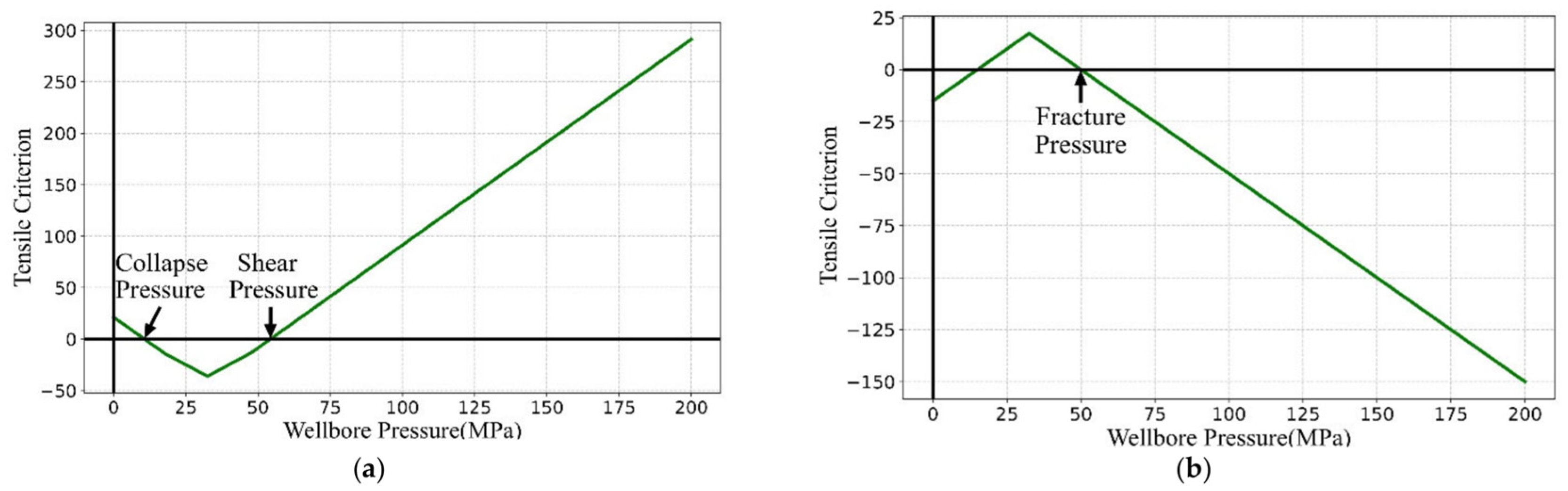
2.3.1. Shear Pressure and Collapse Pressure Based on the M-C Criterion

The M-C criterion is written as follows [31]:

$$\tau ={\sigma }_n\tan \varphi +C,$$

(10)

where $\tau$ and ${\sigma }_n$ are the shear stress and normal stress of the shear plane, respectively, $C$ is the cohesion stress, and $\varphi$ is the internal friction angle. Shear and normal stress can be expressed as follows:

$$\begin{array}{c}\tau ={\displaystyle \frac{1}{2}}\left({\sigma }_1+{\sigma }_2\right)+{\displaystyle \frac{1}{2}}\left({\sigma }_1-{\sigma }_3\right)\cos 2\theta ,\\ {\sigma }_{\mathrm{n}}={\displaystyle \frac{1}{2}}\left({\sigma }_1-{\sigma }_3\right)\sin 2\theta ,\end{array}$$

(11)

where ${\sigma }_1$, ${\sigma }_2$, and ${\sigma }_3$ are the largest principal stress, the next largest principal stress, and the smallest principal stress after principal stresses are sorted. $\theta ={\displaystyle \frac{\pi }{4}}+{\displaystyle \frac{\varphi }{2}}$ is the rock fracture angle. By combining Equation (11) with Equation (10), we can obtain the following:

$${\sigma }_1={\displaystyle \frac{2C\cos \varphi }{1-\sin \varphi }}+{\displaystyle \frac{1-\sin \varphi }{1+\sin \varphi }}{\sigma }_3.$$

(12)

Considering the effective stress theory, Equation (12) can be transformed into the following:

$$f_{\mathbf{m}\mathbf{c}}={\sigma }_1-{\sigma }_3-\sin \left({\sigma }_1+{\sigma }_3-2{\sigma }_{\mathbf{e}}\right)-2C\mathrm{c}\mathrm{o}\mathrm{s}\varphi .$$

(13)

This equation can be written as a quadratic function of $P_W$. Therefore, $P_c$ and $P_s$ are the smaller and larger roots of Equation (13).

2.3.2. Tensile Criterion

When the stress imposed by the drilling mud exceeds the tensile strength of the formations ($T_0$), tensile failure may occur. Here, tensile strength is an intrinsic property of the rock, and the value can be obtained through direct tensile testing [32] or estimated indirectly [33]. Tensile failure typically arises as the smallest effective principal stress exceeds the tensile strength of the formation rock. This criterion can be approximated using the following expression:

$$f_{ts}={\sigma }_3-P_P-T_0.$$

(14)

2.3.3. Determination of Mud Safety Density Window

According to the previous analysis, when the pressure of the drilling fluid column in the well is too low ($P_W<P_c$), the well wall is likely to collapse. Excessively high drilling mud density imposes excessive pressure on the well wall ($P_W>P_s (P_f )$), leading to localized shear stress concentrations in the rock that cause shear failure, as well as the development of tensile stress that results in tensile failure [34]. In addition, in order to maintain the stability of the wellbore and prevent blowout, the drilling fluid column pressure must be greater than the formation pore pressure ($P_W>P_P$) [35]. Therefore, the mud safety density $P$ is determined as follows:

$$\min (P_s,P_f)\ge P\ge \max (P_c,P_P).$$

(15)

Equations (13) and (14) can be written as quadratic functions of $P_W$. We can obtain the threshold value of the safe density range of mud by solving these two equations. Specifically, $P_c$ and $P_s$ are the smaller and larger roots of Equation (13), and $P_f$ is the smaller root of Equation (14).

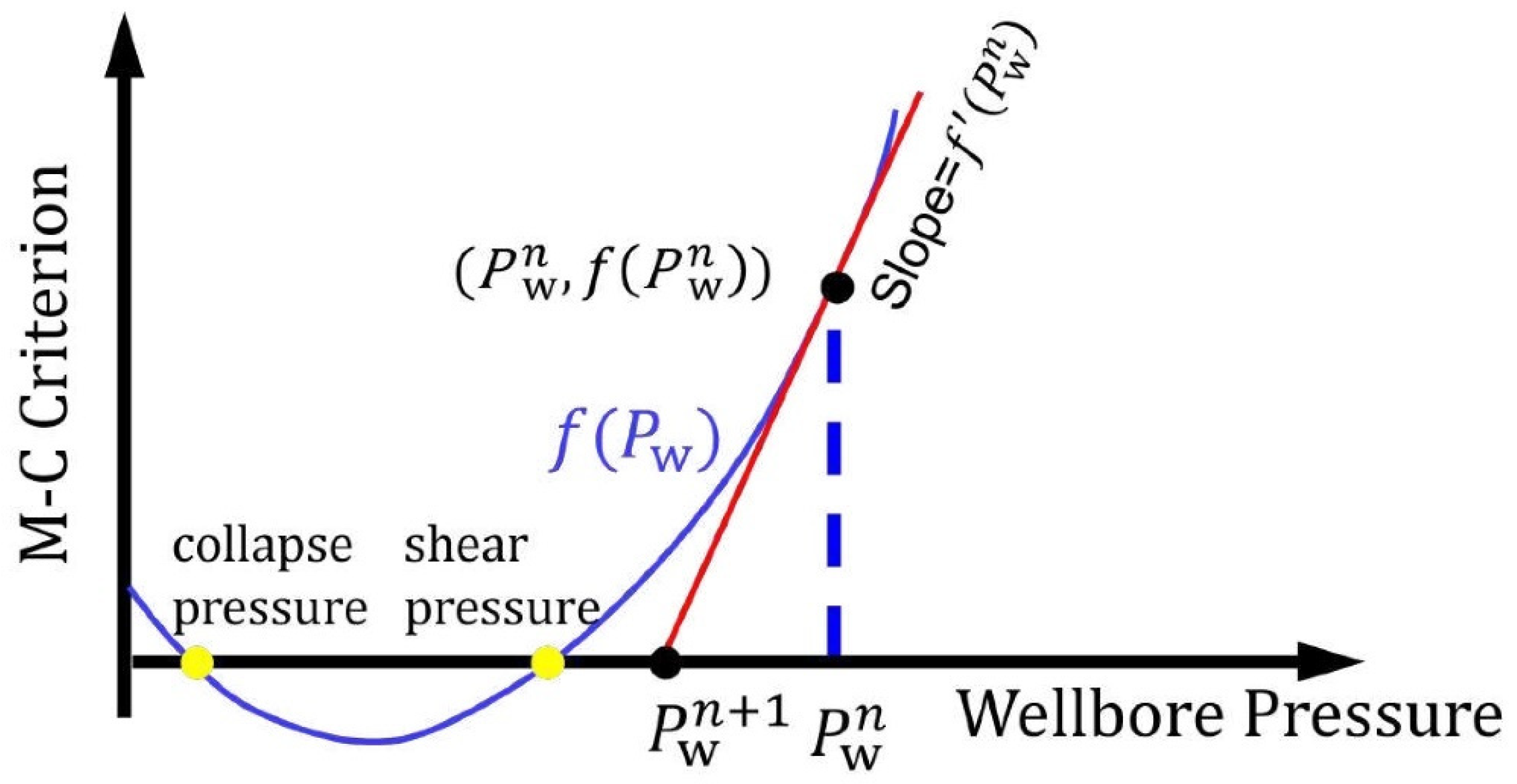
2.4. Calculation of Mud Safety Density Window Based on Newton’s Method

Equations (13) and (14) can be written as quadratic functions of $P_W$. Since quadratic functions are differentiable, we can obtain the threshold value of the safe density range of mud by solving these equations based on Newton’s method. In order to explain these two failure conditions more intuitively, we set up a model for analysis (

Table 1. Parameter values of the formation model.

Parameter	Value	Parameter	Value
$H$	1700 m	${\sigma }_h$	35 MPa
$\alpha$	1	${\sigma }_v$	40 MPa
$\varphi$	30°	St	5 MPa
$P_P$	20 MPa	$v$	0.25
${\sigma }_H$	45 MPa	$\delta$	0%

). Pw is set to range from 0 to 200 MPa, and the criterion value varies with $P_W$, as shown in Figure 2. For the M-C criterion, analyzing collapse pressure and shear pressure, the quadratic function exhibits a downward-facing parabolic curve (Figure 2a). However, the quadratic function for analyzing fracture pressure under the tensile failure criterion has an upward-facing parabolic shape (Figure 2b). Therefore, using Newton’s method, we can precisely solve these two criteria—the M-C criterion for collapse pressure and shear pressure and the tensile failure criterion for fracture pressure. This will allow us to obtain accurate threshold values for the safe mud density window.

It is important to note that this model does not account for the presence of faults, which can significantly influence drilling operations and safety. The strength of fault planes is generally lower than that of ordinary rocks, and if a fault plane intersects obliquely with the model, both the upper and lower limits of the safe drilling fluid density window may decrease. This limitation should be considered when interpreting the results of our study.

In numerical criterion analysis, Newton’s method [36] is a root-finding algorithm which produces successively better approximations of the roots (or zeroes) of a real-valued function. Since both the M-C criterion and the tensile failure criterion involve solving quadratic functions, we can use the solution process of the shear pressure under the M-C criterion as an example to demonstrate the application of Newton’s method (Figure 3). The procedure begins with an initial value $P_W^0$, followed by approximating the function using its tangent line $f^{\prime }\left(P_W^0\right)$. Next, the $P_W$-intercept of this tangent line is calculated. This $f^{\prime }\left(P_W^0\right)$-intercept generally serves as a more accurate approximation of the original function’s root compared to the initial value. For the $n$-th iteration, the slope of the criterion $f^{\prime }\left(P_W^0\right)$ is given by the following:

$$f^{\prime }\left(P_{\mathbf{w}}^n\right)={\displaystyle \frac{f\left(P_{\mathbf{w}}^n\right)-0}{P_{\mathbf{w}}^n-P_{\mathbf{w}}^{n+1}}}.$$

(16)

Solving Equation (16) for $P_W^{n+1}$ gives the following:

$$P_{\mathrm{w}}^{n+1}=P_{\mathrm{w}}^n-{\displaystyle \frac{f\left(P_{\mathrm{w}}^n\right)-0}{f^{\prime }\left(P_{\mathrm{w}}^n\right)}}.$$

(17)

This iterative process terminates when $f\left(P_W^n\right)$ satisfies certain conditions. Here, we can set the termination criterion as $\left|f\left(P_W^n\right)\right|<{10}^{-4}$. Therefore, the final shear pressure is calculated as ${ P}_W^n$. Moreover, the initial value is set to 0, and the smaller root of the quadratic equation based on the M-C criterion is iteratively obtained as $P_c$ through Newton’s method. Similarly, the smaller root of the quadratic equation derived from the tensile failure criterion is obtained as $P_f$.

3. Results

In this section, we established three different stress models based on Anderson fault models to analyze the conditions necessary for maintaining borehole stability. Subsequently, we use these models to guide the development of the borehole network in a real-world oilfield.

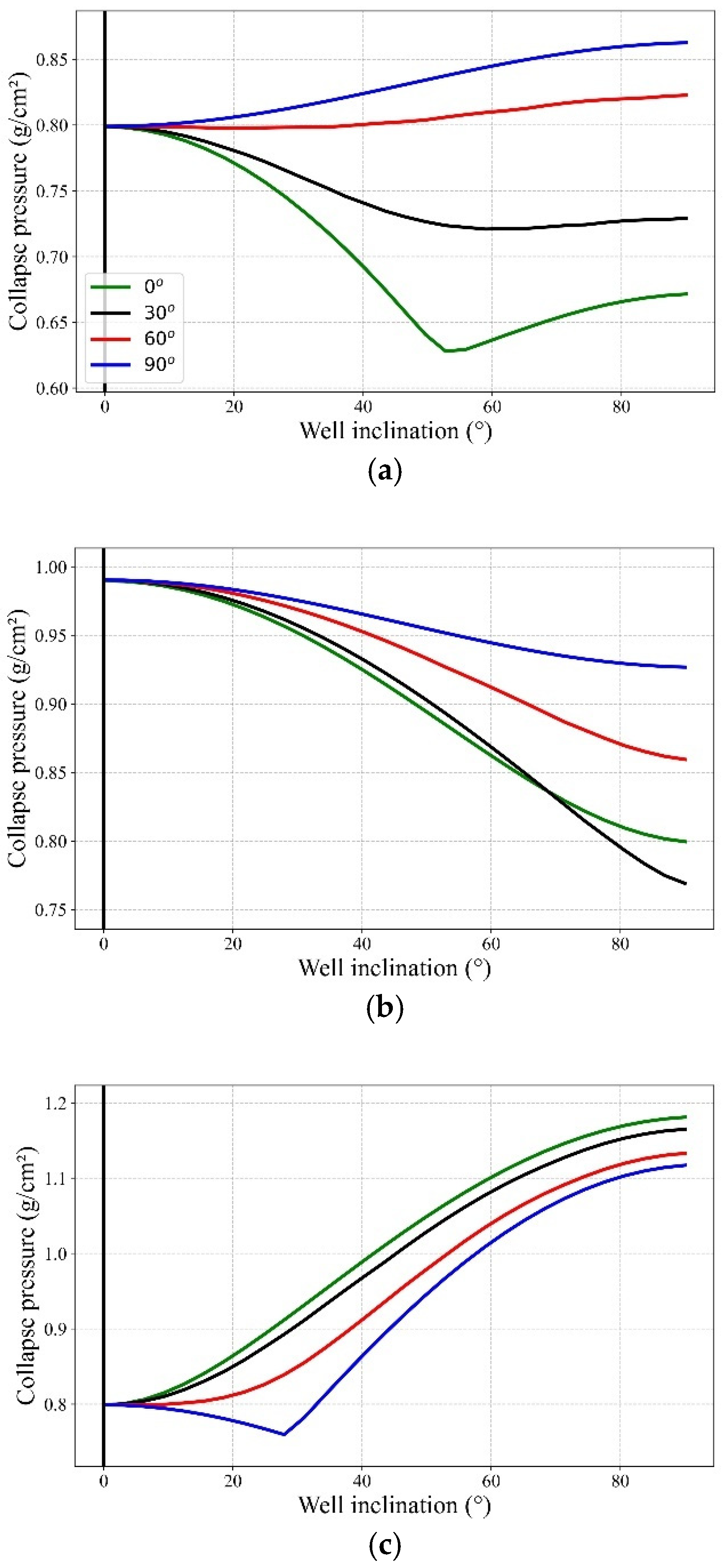
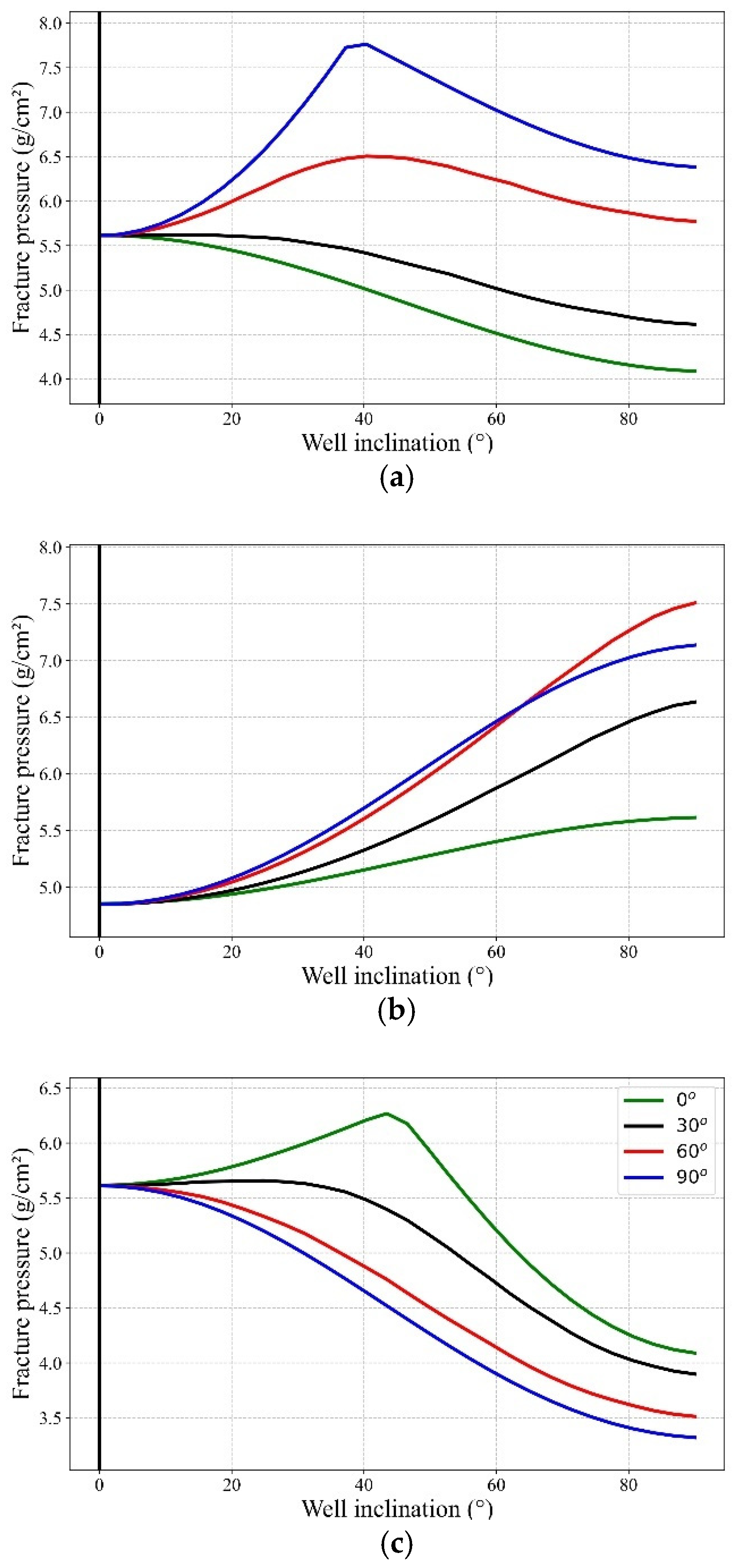
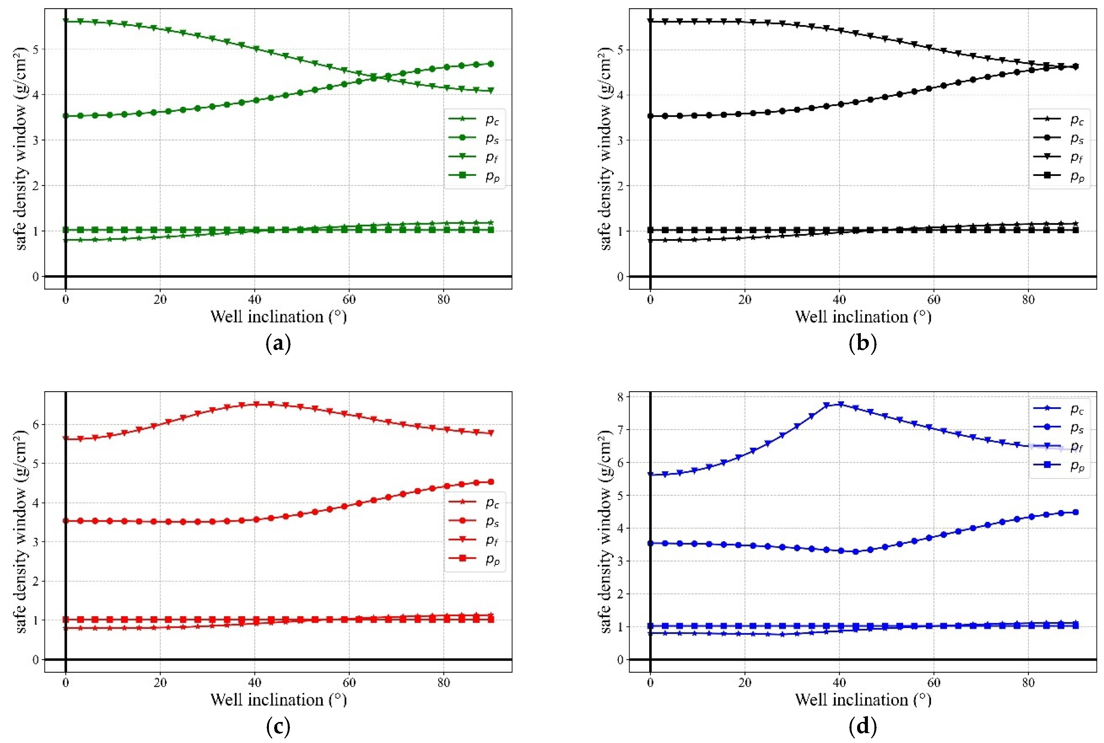
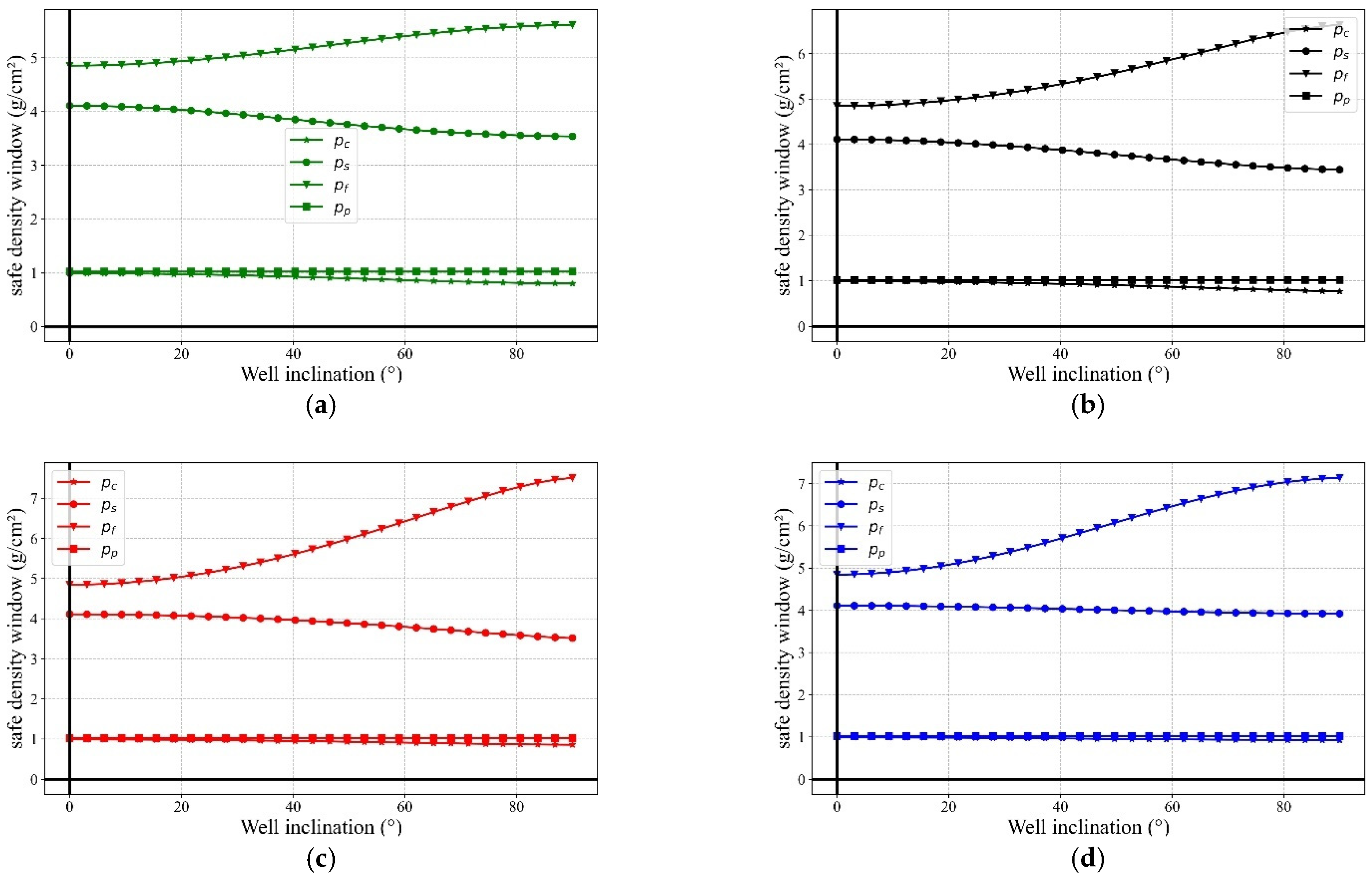
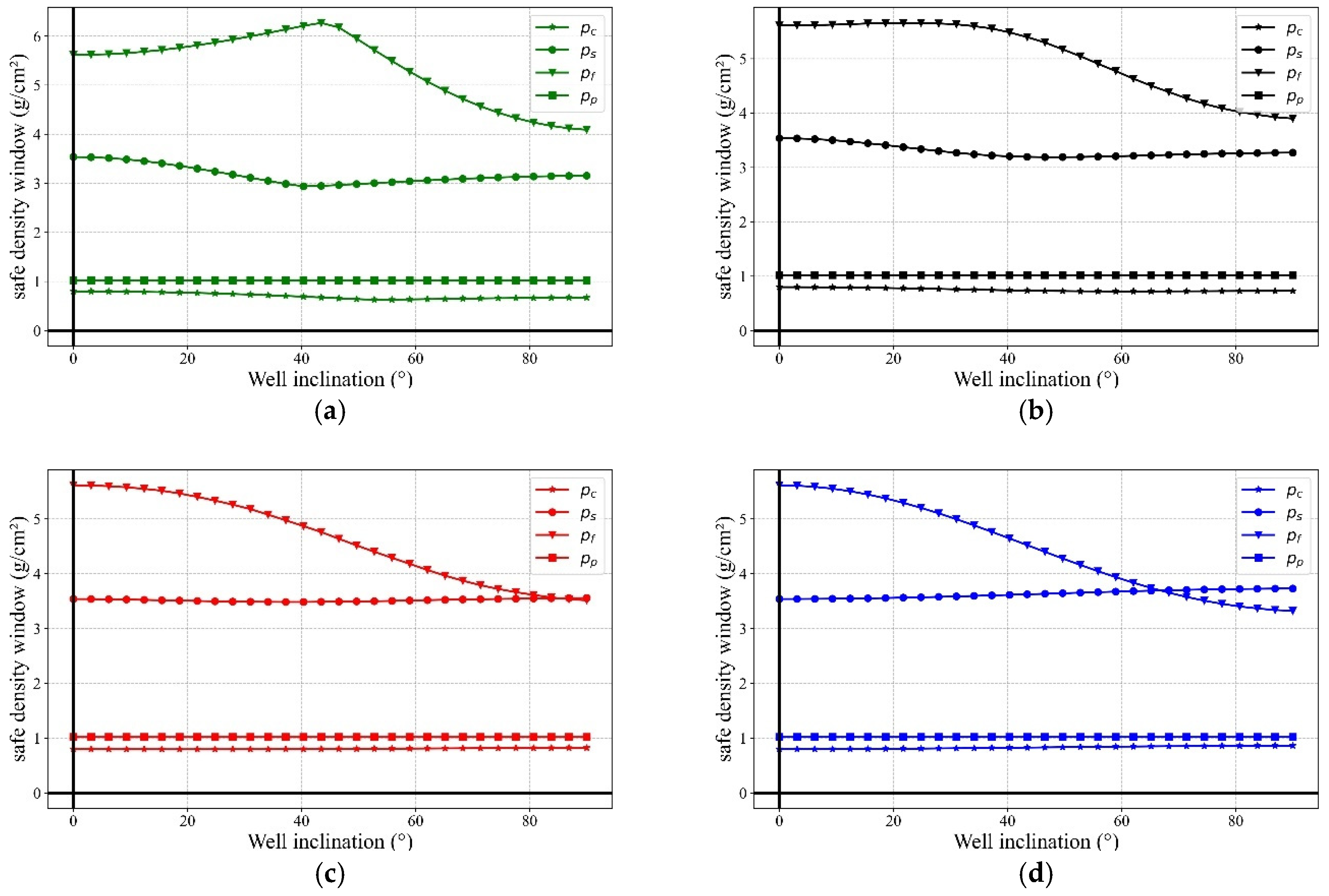
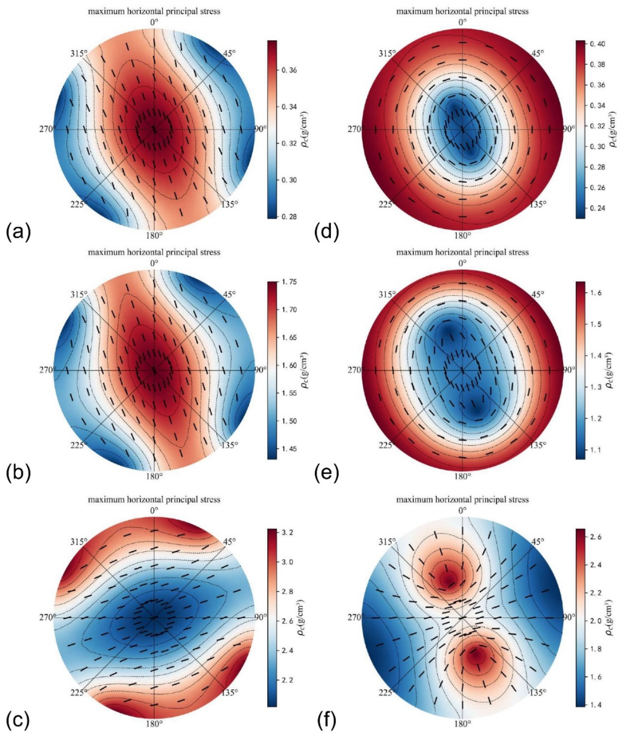
3.1. Safe Mud Density Window Analysis Based on Anderson’s Classification Scheme

In the Cartesian coordinate system, the subsurface medium is primarily subjected to stresses in three directions (Figure 1), including overburden pressure and the maximum and minimum principal stresses in the horizontal direction, which are perpendicular to each other. Anderson’s original framework [37] considers the magnitudes of the greatest, intermediate, and least principal stresses at depth, denoted as $S_1$, $S_2$, and $S_3$, in relation to ${ S}_v$, $S_{Hmax}$, and $S_{hmin}$. The values of horizontal principal stresses can be either less than or greater than the vertical stress, depending on the geological context, as outlined in

Table 2. Faulting regimes under different relative stress magnitudes.

Regime	Stress
	${\mathit{S}}_1$	${\mathit{S}}_2$	${\mathit{S}}_3$
Normal	$S_v$	$S_{Hmax}$	$S_{hmin}$
Strike-slip	$S_{Hmax}$	$S_v$	$S_{hmin}$
Reverse	$S_{Hmax}$	$S_{hmin}$	$S_v$

. Specifically, in normal faulting regimes, the vertical stress $S_v$ corresponds to the maximum principal stress $S_1$; in strike-slip regimes, it represents the intermediate principal stress $S_2$; and in reverse-faulting regimes, it is associated with the least principal stress $S_3$.

In order to analyze the relationship between the wellbore trajectory and the safe mud density window of drilling construction under various stress conditions and to provide a reference for the construction plan and ensure safe drilling construction, three groups of corresponding fault-type models were set up, as shown in

Table 3. Designed parameters of each model.

	${\mathit{S}}_{\mathit{v}}$ (MPa)	${\mathit{S}}_{\mathit{H}\mathit{m}\mathit{a}\mathit{x}}$ (MPa)	${\mathit{S}}_{\mathit{h}\mathit{m}\mathit{i}\mathit{n}}$ (MPa)
Normal	$50 \left(S_1\right)$	$40 \left(S_2\right)$	$35 \left(S_3\right)$
Strike-slip	$40 \left(S_2\right)$	$45 \left(S_1\right)$	$35 \left(S_3\right)$
Reverse	$30 \left(S_3\right)$	$40 \left(S_1\right)$	$35 \left(S_2\right)$

. The unified calculation condition is listed as follows: $P_P$ = 20 MPa, $\eta$ = 1, $C$ = 18 MPa, $\varphi$ = 30°, $H$ = 2000 m, $v$ = 0.25, and $\beta$ is 0° (North–South). Since pressure is axisymmetric, we analyzed the results for azimuth angles ranging from 0° to 90° using the density formula $\rho =P/gh$.

As shown in Figure 4, the collapse pressure varies with well inclination at different azimuth angles. In a normal fault regime, there is a positive correlation between collapse pressure and the well inclination angle. This indicates that a vertically drilled well is generally more structurally stable than a deviated wellbore. Additionally, when the well inclination angle remains constant, collapse pressure exhibits an inverse relationship with the azimuth angle, suggesting that aligning the wellbore orientation with the direction of the minimum horizontal principal stress is typically safer.

In the case of a strike-slip fault state, collapse pressure decreases as the well inclination angle increases while it remains independent of the well inclination angle itself. This makes this stress state more favorable for drilling deviated and horizontal wells. Conversely, in a reverse-fault state, collapse pressure shows a positive correlation with the azimuth angle. However, the relationship between collapse pressure and the well’s inclination angle can vary, potentially increasing or decreasing depending on the specific stress conditions.

Therefore, when designing the trajectory of an inclined wellbore in a reverse fault regime, a thorough analysis of the geomechanical parameters is crucial to ensure wellbore stability. Both shear pressure and collapse pressure are calculated using Equation (13). Consequently, the variation in shear pressure with the well’s inclination (Figure 5) aligns with the changes in collapse pressure with the well’s inclination (Figure 4).

As illustrated in Figure 6, fracture pressure at different azimuth angles changes with the well’s inclination. Under a normal fault state, the fracture pressure exhibits a positive correlation with the azimuth angle while remaining largely uncertain to changes in the wellbore inclination angle. Consequently, by aligning the wellbore trajectory with the direction of the minimum horizontal principal stress, a wider fracture pressure window can be achieved, which is advantageous for wellbore stability. Under the strike-slip fault state, the fracture pressure exhibits a positive correlation with the wellbore inclination angle. However, the fracture pressure does not demonstrate a consistent relationship with the azimuth angle. Consequently, vertically drilled wells are more susceptible to the risk of fracture failure compared to the deviated wellbore. And in the reverse fault state, the variation in fracture pressure is more complex. Generally speaking, the fracture pressure decreases with the increase in azimuth angles.

As shown in Figure 7, Figure 8 and Figure 9, the safe density window varies with the well’s inclination at different azimuth angles across various fault regimes. The green line represents the variation at an azimuth angle of 0°, the black line represents the variation at 30°, the red line represents the variation at 60°, and the yellow line represents the variation at 90°. In these different regimes, the lower limit of the safe density window does not change significantly.

For the upper limit of the safe density window, shear failure occurs under both normal fault and strike-slip fault regimes, irrespective of the azimuth angle. In the normal fault regime, tensile failure is more probable in a highly deviated well that aligns with the direction of the maximum principal stress. Conversely, for reverse fault regimes, as the azimuth angle transitions from the maximum principal stress direction to the minimum principal stress direction, shear pressure increases while fracture pressure decreases.

As illustrated in Figure 7, shear failure occurs when the azimuth angle remains below a certain threshold. Beyond this threshold, an increase in the well inclination angle tends to shift the failure mode from shear to tensile. This shift underscores the importance of carefully considering azimuth and inclination angles when evaluating wellbore stability and designing drilling trajectories.

The preceding analysis presupposes a set of values; however, empirical data are inherently more intricate. The safe density window, particularly its upper boundary, is contingent upon the actual fracture strength and pore pressure gradients. Consequently, these analyses provide significant insights into the refinement of drilling methodologies. In the context of shallow vertical well sections, the determination of the safe mud density window is pivotal to avert wellbore compromise and to establish a foundation for pinpointing the optimal deflection point. For deep-inclined wellbore intervals, a thorough examination of wellbore stability and the delineation of the safe drilling mud density window is imperative. Such an analysis underpins strategies to guarantee drilling operations that are both secure and efficacious.

3.2. Application to Optimize Drilling in Real-World Operations

The oilfield in question is governed by the Tan-Lu Fault Zone, which is predominantly characterized by the development of strike-slip faults [38,39]. The Cenozoic strata, which have accumulated to a thickness of at least 7000 m within the fault subbasins, are delineated by normal faults and, in some areas, by strike-slip faults as well, according to [40]. The region studied is a sedimentary basin rich in oil and gas reserves, marked by intricate fault structures, with strike-slip faults playing a dominant role.

As depicted in Figure 10a–c, the coherence of frequency decomposition of seismic data in certain areas of this oilfield is displayed from shallow to deep using a three-primary-color scheme: red–green–blue. Red represents a relatively low frequency, green indicates a medium frequency, and blue signifies a high frequency. A legend is included in Figure 10a to clarify the physical property parameters represented by each color block. The well, denoted as Well 1, has its planar well trajectory projection illustrated as a black curve line.

Figure 11 presents a profile along the drilling trajectory of the seismic coherence, highlighting distinct flower structures—typical seismic indicators of strike-slip faults [41]. The sectional projection of Well 1 is represented as a blue curved line in Figure 11. In Figure 10, subplots a–c correspond to the shallow layers between the blue and yellow lines, the middle layers between the yellow and purple lines, and the deep layers between the purple and green lines, respectively, in Figure 11.

Numerical simulation results and field data reveal that the direction of the maximum horizontal principal stress is approximately 75° to 80° east of the north. Therefore, the azimuth angle was established at 290°. Figure 12 presents the well-logging data along the measured depth alongside the elastic and rock mechanical parameters. The yellow arrow indicates the strike-slip fault regime, while the red arrow denotes the normal fault regime, corresponding to the color-coded arrows in Figure 11. These arrows identify the strata locations that are particularly vulnerable to leakage. This correlation between the fault regimes and the susceptibility of certain strata emphasizes the importance of understanding the stress orientations and geological conditions when evaluating wellbore stability and potential leakage risks.

Pore pressure, as an isotropic stress, is uniform in all directions. Consequently, the constraints of the safe mud density window are illustrated in Figure 13. This figure depicts the distribution of $\psi$ along the radial axis and $\beta$ along the circumferential axis. The center of the circle corresponds to a vertical well at 0° inclination, while the perimeter represents a horizontal well at 90° inclination. The azimuth angle varies along the circumference, with the 0° azimuth aligned with the direction of the maximum horizontal principal stress. The failure azimuths are denoted by short black lines.

(a–c) The collapse pressure, shear pressure, and fracture pressure under a strike-slip fault regime are shown at a measured depth of 2130 m with $P_P$ = 0.287 g/cm³, corresponding to the yellow arrow in Figure 12.

(d–f) The collapse pressure, shear pressure, and fracture pressure under a normal fault regime are shown at a measured depth of 2830 m with $P_P$ = 0.54 g/cm³, corresponding to the red arrow in Figure 12.

As the depth increases, the safe mud density window becomes narrower to prevent blowout, collapse, tensile, and shear failure. Therefore, we provide safe mud density windows for these locations of strata that are prone to leakage. We utilized an interpolation algorithm to pre-set the mechanical and strength parameters of the exploration well at the corresponding position within the formation. Subsequently, we applied this method to determine the mud safety density window, which facilitated the advance preparation of the mud mixture, ensuring the efficiency, safety, and economy of offshore drilling operations.

4. Conclusions

This study provides a thorough analysis of the geological and engineering challenges in drilling deep subterranean environments. We evaluated borehole stability, formation stress distribution, and risks such as lost circulation and blowouts. The safe mud density window is defined with the lower limit as the smaller value between the pore pressure and collapse pressure and the upper limit as the larger value between the fracture pressure and shear pressure. These pressures were analyzed using the M-C failure criterion and tensile failure, with calculations performed using Newton’s method.

The research integrates Anderson’s classification scheme into stress state analysis, refining its impact on mud density windows. It details how the safe mud density window varies with wellbore inclinations and azimuths, aiding in well trajectory optimization and mitigating instability. This approach allows for precise mud density adjustments in transition zones with varying stress regimes, enhancing drilling safety and reliability.

Finally, applying this method to the studied oilfield, we developed tailored mud density management strategies that could improve borehole stability and safety. In conclusion, this research offers a robust theoretical framework and practical guidelines, highlighting the importance of advanced stress analysis for safer and more efficient deep drilling operations in complex geological settings, contributing to the sustainable exploitation of oil and gas resources.

5. Discussion

In this study, we primarily adopted an isotropic assumption to calculate the mud-weight safety window. However, it is important to recognize that the anisotropic characteristics of geological materials can significantly impact the distribution of in situ stresses and the selection of mud density during actual drilling operations. Anisotropy refers to the directional dependence of physical properties, which is commonly observed in many geological formations, particularly in environments with varying mineral compositions and structures.

Considering the actual data from the Bohai Sea region, the anisotropic nature of the formations may lead to non-uniform stress distributions, thereby affecting wellbore stability and the calculations of the mud-weight safety window. Therefore, future research should aim to incorporate anisotropy into models to more accurately assess variations in mud-weight windows. This approach could enhance the reliability of the computed results and provide stronger support for engineers’ decision-making in complex geological conditions. By delving into the implications of anisotropy, we hope to offer more comprehensive guidance for drilling engineering, ultimately improving the safety and efficiency of drilling operations.

Additionally, while this study focuses on the assumption that the vertical principal stress is directed vertically downward, we acknowledge that geostress conditions can be complex, and the vertical principal stress may tilt, particularly in the presence of geological features such as folds or faults. This assumption facilitates a clearer understanding of the fundamental mechanics involved. We recommend that future research explore the implications of varying principal stress orientations on stress distribution, as this could further enhance our understanding of wellbore stability in more complex geological settings.

References

1. Mohiuddin, M.; Khan, K.; Abdulraheem, A.; Al-Majed, A.; Awal, M.R. Analysis of wellbore instability in vertical, directional, and horizontal wells using field data. J. Pet. Sci. Eng. 2007, 55, 83–92. [Google Scholar] [CrossRef]
2. Li, Q.; Liu, J.; Wang, S.; Guo, Y.; Han, X.; Li, Q.; Cheng, Y.; Dong, Z.; Li, X.; Zhang, X. Numerical insights into factors affecting collapse behavior of horizontal wellbore in clayey silt hydrate-bearing sediments and the accompanying control strategy. Ocean Eng. 2024, 297, 117029. [Google Scholar] [CrossRef]
3. Li, Q.; Li, Q.; Cao, H.; Wu, J.; Wang, F.; Wang, Y. The Crack Propagation Behaviour of CO2 Fracturing Fluid in Unconventional Low Permeability Reservoirs: Factor Analysis and Mechanism Revelation. Processes 2025, 13, 159. [Google Scholar] [CrossRef]
4. Peška, P.; Zoback, M. Compressive and tensile failure of inclined well bores and determination of in situ stress and rock strength. J. Geophys. Res. Solid Earth 1995, 100, 12791–12811. [Google Scholar] [CrossRef]
5. Mireille, C. Essai sur une application des règles de maximis & minimis à quelques problèmes de statique, relatifs à l’architecture. Rev. Fr. Géotech. 2003, 175, 1–43. [Google Scholar] [CrossRef]
6. Declan, G.; Winthrop, D. Mohr circles of the first and second kind and their use to represent tensor operations. J. Struct. Geol. 1984, 6, 693–701. [Google Scholar] [CrossRef]
7. Littke, R.; Sachsenhofer, R.F. Organic petrology of deep sea sediments: A compilation of results from the Ocean Drilling Program and the Deep Sea Drilling Project. Energy Fuels 1994, 8, 1498–1512. [Google Scholar] [CrossRef]
8. Barton, N. The shear strength of rock and rock joints. International Journal of rock mechanics and mining sciences & Geomechanics abstracts. Pergamon 1976, 13, 255–279. [Google Scholar] [CrossRef]
9. Xu, C.G.; Yu, H.B.; Wang, J.; Liu, X. Formation conditions and accumulation characteristics of Bozhong 19-6 large condensate gas field in offshore Bohai Bay Basin. Pet. Explor. Dev. 2019, 46, 27–40. [Google Scholar] [CrossRef]
10. Shi, L.; Jin, Z.K.; Yan, W.; Zhu, X.; Xu, X.; Peng, B. Influences of overpressure on reservoir compaction and cementation: A case from northwestern subsag, Bozhong sag, Bohai Bay Basin, East China. Pet. Explor. Dev. 2015, 42, 339–347. [Google Scholar] [CrossRef]
11. Xu, C.G.; Du, X.F.; Liu, X.J.; Xu, W.; Hao, Y. Formation mechanism of high-quality deep buried-hill reservoir of Archaean metamorphic rocks and its significance in petroleum exploration in Bohai Sea area. Oil Gas Geol. 2020, 41, 235–247, 294. (In Chinese) [Google Scholar]
12. Li, Z.; Xie, R.J.; Wu, Y.; Yuan, J. Progress and prospect of CNOOC’s oil and gas well drilling and completion technologies. Nat. Gas Ind. B 2022, 9, 209–217. [Google Scholar] [CrossRef]
13. Eaton, B.A. The equation for geopressure prediction from well logs. In Proceedings of the SPE Annual Technical Conference and Exhibition, Dallas, TX, USA, 28 September–1 October 1975. [Google Scholar] [CrossRef]
14. Lu, B.P.; Bao, H.Z. Advances in calculation method for rock mechanics parameters. Pet. Drill. Tech. 2005, 33, 44–47. [Google Scholar]
15. Leopold, M. Fundamentals of Rock Mechanics; Springer: Vienna, Austria, 1969; pp. 3–28. [Google Scholar] [CrossRef]
16. Mann, D.M.; Mackenzie, A.S. Prediction of pore fluid pressures in sedimentary basins. Mar. Pet. Geol. 1990, 7, 55–65. [Google Scholar] [CrossRef]
17. Sayers, C.M.; Johnson, G.; Denyer, G. Predrill pore pressure prediction using seismic data. Geophysics 2002, 67, 1286–1292. [Google Scholar] [CrossRef]
18. Zhang, J. Pore pressure prediction from well logs: Methods, modifications, and new approaches. Earth-Sci. Rev. 2011, 108, 50–63. [Google Scholar] [CrossRef]
19. Terzaghi, K. Erdbaumechanik auf Bodenphysikalischer Grundlage. 1925. Available online: https://scispace.com/papers/erdbaumechanik-auf-bodenphysikalischer-grundlage-539sbnypud (accessed on 19 January 2025).
20. Biot, M.A.; Willis, D.G. The elastic coefficients of the theory of consolidation. J. Appl. Mech. 1957, 24, 594–601. [Google Scholar] [CrossRef]
21. Ju, W.; Shen, J.; Qin, Y.; Meng, S.; Wu, C.; Shen, Y.; Yang, Z.; Li, G.; Li, C. In-situ stress state in the Linxing region, eastern Ordos Basin, China: Implications for unconventional gas exploration production. Mar. Pet. Geol. 2017, 86, 66–78. [Google Scholar] [CrossRef]
22. Huang, R.Z. A model for predicting formation fracture pressure. J. Univ. Pet. China 1984, 4, 335–347. [Google Scholar]
23. Thiercelin, M.J.; Plumb, R.A. Core-based prediction of lithologic stress contrasts in east texas formations. SPE Form. Eval. 1994, 9, 251–258. [Google Scholar] [CrossRef]
24. Cao, H.; Zhao, Y.; Shuai, D.; Qi, Y.; Chen, G.; Li, S. Using 3d seismic data to estimate stress based on seismic curvature attribute of HTI medium: Application to the weiyuan, southern sichuan basin, china. J. Geophys. 2024, 67, 1970–1986. (In Chinese) [Google Scholar] [CrossRef]
25. Roberts, A. Curvature attributes and their application to 3d interpreted horizons. First Break 2001, 19, 85–100. [Google Scholar] [CrossRef]
26. Kirsch, G. Die theorie der elastizität und die bedürfnisse der festigkeitslehre. Z. Des Vereines Dtsch. Ingenieure 1898, 42, 797–807. [Google Scholar]
27. Haimson, B.; Fairhurst, C. In-situ stress determination at great depth by means of hydraulic fracturing. In Proceedings of the 11th U.S. Symposium on Rock Mechanics (USRMS), Berkeley, CA, USA, 16–19 June 1969. [Google Scholar]
28. Hiramatsu, Y. Stress Around a Shaft or Level Excavated in Ground with a Three-Dimensional Stress State; Memoirs of the Faculty of Engineering, Kyoto University: Kyoto, Japan, 1962; Volume 24, Available online: http://hdl.handle.net/2433/280512 (accessed on 18 January 2025).
29. Hiramatsu, Y.; Oka, Y. Determination of the stress in rock unaffected by boreholes or drifts, from measured strains or deformations. Int. J. Rock Mech. Min. Sci. Geomech. Abstr. 1968, 5, 337–353. [Google Scholar] [CrossRef]
30. Bradley, W.B. Failure of inclined boreholes. J. Energy Resour. Technol. 1979, 101, 232–239. [Google Scholar] [CrossRef]
31. Labuz, J.; Zang, A. Mohr-coulomb failure criterion. In The ISRM Suggested Methods for Rock Characterization, Testing and Monitoring; Springer: Berlin/Heidelberg, Germany, 2015; pp. 227–231. [Google Scholar] [CrossRef]
32. Hobbs, D. The tensile strength of rocks. Int. J. Rock Mech. Min. Sci. Geomech. Abstr. 1964, 1, 385–396. [Google Scholar] [CrossRef]
33. Hoek, E. Fracture of anisotropic rock. J. S. Afr. Inst. Min. Metall. 1964, 64, 501–518. [Google Scholar]
34. Pašić, B.; Gaurina, M.; Matanović, D. Wellbore instability: Causes and consequences. Rud.-Geološko-Naft. Zb. 2007, 19, 87–98. Available online: https://hrcak.srce.hr/19296 (accessed on 18 January 2025).
35. Li, S.; George, J.; Purdy, C. Pore-pressure and wellbore stability prediction to increase drilling efficiency. J. Pet. Technol. 2012, 64, 98–101. [Google Scholar] [CrossRef]
36. Galántai, A. The theory of newton’s method. J. Comput. Appl. Math. 2000, 124, 25–44. [Google Scholar] [CrossRef]
37. Anderson, E.M. The Dynamics of Faulting and Dyke Formation with Applications to Britain; Oliver and Boyd: Edinburgh, UK, 1997. [Google Scholar] [CrossRef]
38. Allen, M.B.; Macdonald, D.; Zhao, X.; Vincent, S.J.; Brouet-Menzies, C. Early Cenozoic two-phase extension and late Cenozoic thermal subsidence and inversion of the Bohai Basin, northern China. Mar. Pet. Geol. 1997, 14, 951–972. [Google Scholar] [CrossRef]
39. Hsiao, L.Y.; Graham, S.A.; Tilander, N. Seismic reflection imaging of a major strike-slip fault zone in a rift system: Paleogene structure and evolution of the Tan-Lu fault system, Liaodong Bay, Bohai, offshore China. AAPG Bull. 2004, 88, 71–97. [Google Scholar] [CrossRef]
40. Ye, H.; Shedlock, K.M.; Hellinger, S.J.; Sclater, J.G. The north China basin: An example of a Cenozoic rifted intraplate basin. Tectonics 1985, 4, 153–169. [Google Scholar] [CrossRef]
41. Christie, B.N.; Biddle, K. Deformation and Basin Formation Along Strike-Slip Fault; SEPM Special Publications: Claremore, OK, USA, 1985; SP 37. [Google Scholar]
Figure 1. Polar coordinate transformation of stresses in an inclined well.
Processes 13 01046 g001
Figure 2. Relationship between wellbore pressure and failure criterion. (a) M-C criterion, and (b) tensile failure criterion.
Processes 13 01046 g002
Figure 3. Illustration of solving the M-C criterion to calculate shear stress and collapse pressure using Newton’s method.
Processes 13 01046 g003
Figure 4. Collapse pressure as a function of well inclination at different azimuth angles under various stress regimes: (a) normal fault, (b) strike-slip fault, and (c) reverse fault.
Processes 13 01046 g004
Figure 5. Shear pressure as a function of the well’s inclination at different azimuth angles under various stress regimes: (a) normal fault, (b) strike-slip fault, and (c) reverse fault.
Processes 13 01046 g005
Figure 6. Fracture pressure as a function of the well’s inclination at different azimuth angles under various stress regimes: (a) normal fault, (b) strike-slip fault, and (c) reverse fault.
Processes 13 01046 g006
Figure 7. Safe density window as a function of the well’s inclination at different azimuth angles under normal fault regimes: (a) 0°, (b) 30°, (c) 60°, and (d) 90°.
Processes 13 01046 g007
Figure 8. Safe density window as a function of the well’s inclination at different azimuth angles under strike-slip fault regimes: (a) 0°, (b) 30°, (c) 60°, and (d) 90°.
Processes 13 01046 g008
Figure 9. Safe density window as a function of the well’s inclination at different azimuth angles under reverse fault regimes: (a) 0°, (b) 30°, (c) 60°, and (d) 90°.
Processes 13 01046 g009
Figure 10. The three-primary-color scheme displays the coherence of frequency decomposition of seismic data for faults and fractures in certain areas of the studied oilfield from shallow to deep zones: (a) shallow depth, (b) middle depth, and (c) deep depth. The color scheme is as follows: red represents relatively low frequency, green indicates medium frequency, and blue signifies high frequency.
Processes 13 01046 g010
Figure 11. A joint display of the seismic wave profile, horizon line, and fault recognition. The blue, yellow, and green curve presents horizon line. The pink curve is the fault recognition result, and the yellow arrow indicates the strike-slip fault regime, while the red arrow denotes the normal fault regime.
Processes 13 01046 g011
Figure 12. Well-logging data of a specific well in the studied oilfield. The yellow arrow presents the depth in the strike-slip fault regime, and the red arrow denotes the depth in the normal fault regime.
Processes 13 01046 g012
Figure 13. The limitation of the safe mud density window varies with different fault regimes at various depths, with the failure azimuth angle illustrated by short black lines. (ac) The collapse pressure, shear pressure, and fracture pressure are shown under a strike-slip fault regime at a measured depth of 2130 m with P P = 0.287 g/cm3, corresponding to the yellow arrow in Figure 12. (df) The collapse pressure, shear pressure, and fracture pressure are shown under a normal fault regime at a measured depth of 2830 m with P P = 0.54 g/cm3, corresponding to the red arrow in Figure 12.
Processes 13 01046 g013