Machine Learning-Based Sizing Model for Tapered Electrical Submersible Pumps Under Multiple Operating Conditions

Abstract

Dewatering gas wells typically exhibit a high gas–liquid ratio, making tapered electrical submersible pump (ESP) systems a common choice. However, the flow rate within the pump varies significantly along its length, and production parameters fluctuate considerably across different stages of operation for a gas reservoir. Traditional ESP sizing methods typically consider one single operating case and one single pump model. In contrast, tapered ESP systems require the designer to manually select and combine pump models, stage numbers, and operating frequencies based largely on experience. This process can be cumbersome and time-consuming. To address the limitations of existing ESP sizing methods, this study develops a computational program for ESP operation parameters stage by stage and generates extensive training data. A fully connected neural network (FCNN) based on the backpropagation (BP) algorithm is then trained on these data. The model can predict key parameters such as gas volume fraction (GVF) and flow rate along the pump, operating frequency, and total pump efficiency, using input data such as fluid parameters at the pump’s intake and discharge, as well as pump stage numbers and performance curve data. The model demonstrates high accuracy, with a mean absolute error (MAE) of 0.3431, a mean squared error (MSE) of 0.3231, and a coefficient of determination (R²) of 0.9991. By integrating a wellbore two-phase flow model and leveraging industry experience in pump sizing, a hybrid model for automatic ESP sizing under multiple working conditions is proposed, with the objective of maximizing pump efficiency. This model enables optimal pump sizing, calculates the operating frequency corresponding to given working cases, significantly reduces the workload of designers, and enhances the overall design outcomes.

1. Introduction

The electrical submersible pump (ESP) system offers flexibility in adjusting production parameters, generating significant economic benefits, and has thus been widely adopted [1]. In recent years, it has found extensive application in gas well dewatering applications due to its ability to accommodate high liquid production rates and substantially reduce bottom hole pressure during drainage and gas production [2,3,4,5].

Recent studies have also focused on the challenges of ESP operation in high gas–liquid ratio (GLR) conditions. The flow rate within the pump fluctuates considerably due to the gas compression caused by the stage-by-stage pressurization within the pump. As a result, a tapered ESP system is required [6,7]. A schematic of its structure is shown in Figure 1. In such systems, a multiphase flow pump with a higher nameplate flow rate is typically used as the lower pump, while a conventional pump with a lower nameplate flow rate is usually employed as the upper pump [8,9]. Designers need to consider the appropriate combination of pump models and stage numbers. Moreover, for most gas reservoirs, the daily liquid and gas production rates of the same gas well can vary significantly over time, making the sizing procedure even more challenging.

Traditional ESP sizing procedures [10] usually consider only one single operating condition and one single pump model. However, in gas well dewatering applications, the applicability of two ESP models under multiple working conditions must be evaluated. The choice of pump models and stage numbers affects the operating frequency under each working condition, which in turn impacts the operating efficiency of each pump. This iterative process complicates the sizing of the pump model and stage number combination.

In 2024, Yao [11] proposed an automatic sizing method for tapered ESP under multiple working conditions. This method ensures that the flow rates fall within the recommended operating range for each pump. The method analyzes the intake and discharge conditions and the connection points of the two pumps as design nodes. The node data, calculated based on the preset working conditions, are used as design parameters. The tapered pump selection is performed from the bottom up. After designing the lower pump, the parameters for the upper nodes are updated for the selection of the upper pump. Once all pump models are designed, the operating frequency under the preset working conditions is calculated to determine if the design falls within the recommended operating range. If the conditions are met, the design is complete; otherwise, a redesign with alternative pump models is required. This method addresses the complex task of automatic sizing of tapered ESP under multiple working conditions. It can automatically select a reasonable pump model and stage number combination and calculate the corresponding operating frequencies for different working conditions.

However, this approach has certain limitations. It only uses the flow rate range of each pump section as a constraint without considering the optimization of pump efficiency. Additionally, the pump head is calculated based on the average flow rate in the pump rather than stage-by-stage calculations, leading to potential errors. Furthermore, the method requires substantial computational resources, as it generates all feasible pump models and stage number combinations, leading to long calculation times.

Machine learning is gradually playing an important role in the oil industry, especially in the field of ESP, including flow rate estimation [12], ESP fault diagnosis [13,14,15], lifespan prediction [16], operating parameters optimization [17,18], etc. It is becoming an important tool for improving oil production efficiency. However, there is no study on applying machine learning algorithms to the sizing job of tapered ESP systems.

This paper proposes a stage-by-stage simulator for the tapered ESP system, which generates extensive calculation data. These data are then used to train a fully connected neural network (FCNN) model based on the backpropagation (BP) algorithm. The model’s input parameters include surface liquid production, the tubing GLR, pump intake and discharge pressures, and ESP performance curves and stages. The output parameters include overall pump efficiency, intake and discharge flow rates, gas volume fractions (GVF) for each pump, and operating frequency. The machine learning model is integrated with empirical models, such as the wellbore two-phase flow model and the ESP sizing empirical rules, to form a hybrid model for automatic sizing of tapered ESP system under multiple working conditions with the goal of optimizing pump efficiency. This hybrid model can quickly calculate parameters for various pump models and stage number combinations, enabling the identification of configurations that maximize pump efficiency, thus providing valuable insights for ESP sizing.

This study addresses the following key challenges: the integration of machine learning with empirical models to optimize tapered ESP systems under multiple operating conditions and the improvement of computational efficiency in ESP sizing while maintaining high prediction accuracy. By addressing these challenges, this work provides a robust and efficient framework for tapered ESP sizing, reducing the reliance on manual design and enhancing overall system performance.

2. Overview of ESP Hybrid Sizing Model

2.1. Conventional Design Methods

The traditional ESP sizing method is based on the nodal analysis method [19]. It is generally based on a set of design conditions (including liquid/gas production, reservoir inflow performance, wellbore structure, wellhead pressures, and other parameters), calculates the pressure difference between the pump discharge and intake, selects a reasonable pump model according to the fluid production rate, obtains the single-stage head through the performance curve, and calculates the required stage number.

Firstly, calculating the pump intake parameters, gas reservoir numerical simulation is used to calculate the bottom hole flowing pressure under each set of preset conditions; then wellbore two-phase flow calculation models are used, such as the Beggs–Brill model [20], to calculate the intake pressure. Assuming that the liquid phase is incompressible water and the gas phase is natural gas, the gas volume under certain conditions can be calculated by pressure, temperature, and gas compression factor [21,22]. And the gas compression factor under the given condition can be calculated with the Hall–Yarborough model; the calculation formula is as follows [23]:

$$Z=\left[{\displaystyle \frac{0.06125p_{r}t}{Y}}\right]\mathit{exp}\left[-1.2{\left(1-t\right)}^2\right]$$

(1)

where Z is the gas compression factor, dimensionless, p_r is the relative pressure, MPa; t is the inverse of the relative temperature, and K⁻¹; Y is the relative density, dimensionless.

According to the fluid flow rate, GVF, and other information, a reasonable gas–liquid separator is selected to obtain the separator separation efficiency. The pump intake gas flow rate after the separator is calculated using the separator separation efficiency to obtain the gas/liquid phase volume flow rate, GVF, and other data at the pump intake. The pump intake working condition calculation is completed.

Secondly, the pump discharge parameters are calculated. According to the gas and liquid phase flow rate in the tubing and the wellhead tubing pressure, the wellbore two-phase flow calculation model is used to calculate the pressure and other data at the pump discharge.

When only one type of pump is used, the designer shall select the appropriate pump model according to the flow rate, then determine the single-stage head according to the pump flow rate and the performance curve at the design frequency; finally, the designer shall determine the number of stages according to the ratio of the total dynamic head to the single-stage head.

When designing a tapered pump, the designer usually needs to determine the design operating frequency based on experience; select the two pump models based on the fluid volume flow rate at the pump intake discharge; and manually design the corresponding stage numbers of each pump. After the pump model and stage number combination are completed, the operating frequency under each given working condition is calculated. Pump model selection and stage number sizing usually rely on the designer’s experience. Due to the large number of pump models and stage number combinations, it is extremely difficult to determine the optimal combination.

2.2. Hybrid Model Framework

Based on the above analysis, the main calculation steps to achieve the optimal design of tapered ESP efficiency under multiple working conditions are as follows:

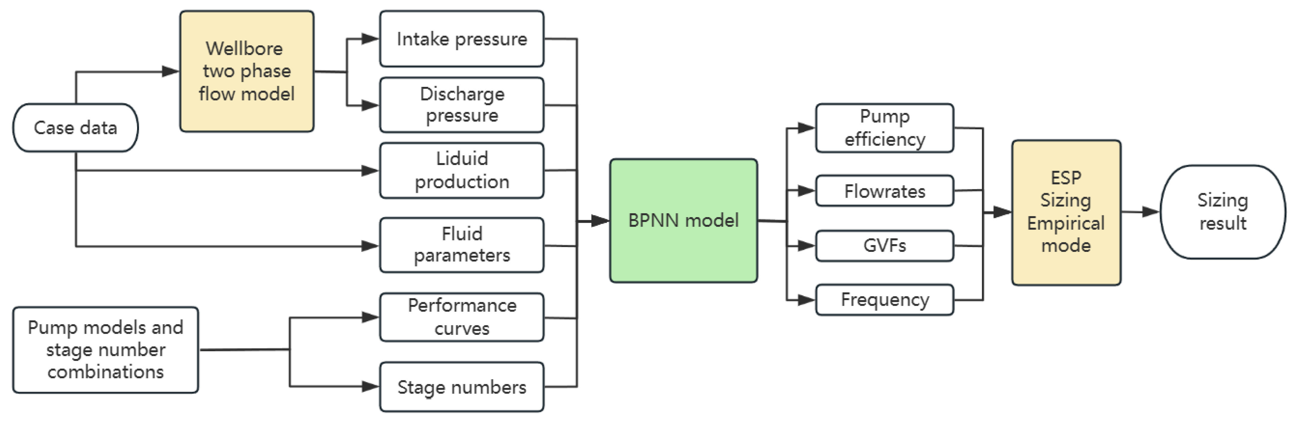
• Wellbore two-phase flow calculation: Using the gas reservoir numerical simulation results, the bottom hole flowing pressure for each given working condition is determined. This pressure serves as the starting point to calculate the pump intake parameters (before the separator) under each working condition using the wellbore two-phase flow calculating model, including total fluid flow, pressure, and GVF. A reasonable separator is then selected, and the separating efficiency is determined. Then, the pump intake (after the separator) parameters are calculated. Then, using the wellbore two-phase flow model, the pump discharge data under each working condition are calculated, starting from the wellhead tubing pressure.
• Pump efficiency calculation: After obtaining the pump intake and discharge working data, the stage-by-stage pump calculation model is used to calculate pump efficiency, operating frequency, and other data for the inlet and outlet of each pump under different pump models and stage number combinations.
• Pump selection and optimization: The primary objective of this process is to eliminate designs that may cause operational failures and to maximize the overall pump efficiency of tapered ESP systems under multiple operating conditions. To avoid operational failures, the key constraints include GVF inside two pumps that must be below the pump limit to prevent gas locking; and the operating frequency must remain within a certain range to ensure proper lubrication and avoid increased equipment costs. To maximize the pump efficiency, each operating condition is assigned a weight, and the pump efficiency is calculated as a weighted average; the weighted average efficiencies for various pump models and stage numbers are then compared to determine the optimal combination of the pump model and stage number.

According to the procedure above, the number of calls to the wellbore two-phase flow model in step 1 is the number of working conditions. The calculation load is relatively small, so a machine learning model is not necessary at this stage. In step 2, the number of calls to the pump stage-by-stage calculation model depends on the number of ESP models and the range of stages. The calculation load is high in this step. For example, if there are 10 types of multiphase pump models and 10 types of conventional pump models in the ESP database, with stage ranges from 101 to 200, the calculation program needs to be called 1,000,000 times to cover all combinations of pump models and stage numbers. In actual applications, the number of pump models and stage ranges will be even larger, resulting in even higher computational demands. Therefore, a machine learning model is suited for speeding up the calculation process in this step. In step 3, since it only involves screening data obtained from step 2 and calculating weighted averages, the computational load is small, and a machine learning model is not required.

Based on the above analysis, the process for the hybrid model is as follows: Firstly, the wellbore two-phase flow model is used to calculate the pump intake and discharge parameters under various working conditions. Then, the FCNN model is used to calculate the ESP operating frequency, flow rate, GVF, and total pump efficiency for each pump model and stage number combination under each given operating condition. Finally, the empirical ESP sizing rules are applied to filter out invalid designs, and the remaining designs are sorted according to weighted pump efficiency to obtain the final selection results.

The structural diagram of the hybrid model for tapered ESP sizing under multiple working conditions is shown in Figure 2.

2.3. ESP Sizing Empirical Model

In conjunction with the conventional ESP sizing method, before determining the final tapered ESP design, it is necessary to screen all results calculated by the FCNN model. The specific steps are as follows:

• GVF constraint: The constraint of filtering out designs with a gas volume fraction (GVF) exceeding 30% [24,25,26] at the intake of the upper pump is based on well-established engineering principles and field experience. Conventional pumps with mixed-flow designs are not capable of handling high GVF conditions efficiently, as excessive gas content can lead to gas locking, reduced pump efficiency, and even operational failure. By excluding such designs, we ensure that the selected pump configurations operate within their recommended performance range, thereby maintaining high efficiency and reliability.
• Frequency range: The minimum operating frequency of all working conditions should not be less than 35 Hz. Based on field experience, ESP systems should run under a frequency of at least 35 Hz to ensure proper lubrication of the seal bearing and prevent failure. The maximum operating frequency of all working conditions should be close to the design frequency. When the design frequency is set at 60 Hz, in some cases, the pump model and stage number combination with the highest weighted pump efficiency may result in a maximum operating frequency significantly lower than 60 Hz. While this design may provide higher pump efficiency, it can also lead to a higher number of ESP stages and increased equipment costs, which is not optimal. Therefore, the model restricts the maximum operating frequency range to 59–60 Hz across all working conditions. The model is flexible in adjusting this frequency range to accommodate specific field conditions. Users can modify the lower frequency limit and design frequency within the model’s input parameters, allowing for customization based on well-specific requirements or operational constraints. For example, in wells with lower liquid production rates, the lower frequency limit can be reduced to 30 Hz, while in high-flow-rate wells, the design frequency can be increased to 70 Hz [27].
• Weighted averaging of pump efficiencies: After screening, the ESP operating conditions are assigned weights based on factors such as condition duration. The objective function for the optimization is defined as the maximization of the weighted pump efficiency across all operating conditions. Mathematically, the objective function can be expressed as the following:

  $${\eta }_{weighted}={\sum }_1^n{w}_i{·\eta }_i$$

  (2)

  where n is the total number of operating conditions, η_weighted is the weighted pump efficiency, fraction; η_i is the total pump efficiency for working condition i, fraction; and w_i is the weight assigned to the operating condition i, reflecting its relative importance. This objective function ensures that the optimization process prioritizes designs that perform well under the most critical operating conditions while maintaining high efficiency across all scenarios.

3. Tapered ESP Operating Parameters FCNN Model

3.1. Mechanism Model for Calculating the Operating Parameters of Tapered ESP

The input parameters for the model include pump intake and discharge pressure, surface liquid production, surface water and gas production, tubing GLR, gas and water relative densities, fluid temperature in the pump, and the head and efficiency performance curves for both the upper and lower pumps. The performance curve is usually in the form of a series of flow rates corresponding to the head and efficiency, so the head and efficiency performance curves must be parameterized so that they can be used as input variables. The method of parameterizing the performance curves in this model involves using the flow rate as the independent variable and the head and efficiency as dependent variables. These curves are then fitted to a quintic equation [28], and the coefficients derived from this fitting process are used as the parameters in the model input.

The operating frequency of the ESP is determined using the dichotomy method. Once the operating frequency is obtained, the remaining operational parameters of the ESP are calculated.

The calculation process for the ESP operation parameter model is as follows:

(1)

Set initial frequencies f₁ and f₂ to 0 Hz and 100 Hz, respectively.

(2)

Calculate the median value of f₁ and f₂, denoted as f₃, and use the ESP affinity law [11] to calculate the head and efficiency performance curves for the two pumps under f₃.

(3)

Perform stage-by-stage calculations in the pump. Starting from the pump intake, obtain the head of the first-stage pump based on the pump intake flow rate from the performance curve. This is then converted into a pressure boost, and the fluid pressure and flow rate at the outlet of this stage are calculated. These values are used as the intake parameters for the second-stage pump to calculate the discharge pressure and flow rate of the second-stage pump. This step is repeated until the last pump is calculated.

(4)

If the discharge pressure of the last pump exceeds the design discharge pressure, assign the value of f₃ to f₂; otherwise, assign f₃ to f₁.

(5)

If the difference between f₂ and f₁ is less than 0.2 Hz, the final operating frequency is the median value of f₁ and f₂. If the difference is greater than 0.2 Hz, return to step 2 to recalculate.

(6)

For the final operating frequency, perform stage-by-stage calculation and save the flow rate and GVF at the pump intake, the connection point between the two pumps, and the pump discharge. During the stage-by-stage calculation process, the power consumption of each stage is calculated. The power consumption at each stage is then used to calculate the total efficiency of the ESP. The formula for calculating the total pump efficiency is as follows:

$$\eta ={\displaystyle \frac{\sum _1^{n_1+n_2}{\rho }_{i}g{H}_i{Q}_i}{\sum _1^{n_1+n_2}{P}_i}}={\displaystyle \frac{\sum _1^{n_1+n_2}{\rho }_{i}g{H}_i{Q}_i}{\sum _1^{n_1+n_2}{\rho }_{i}g{H}_i{Q}_i/{\eta }_i}}$$

(3)

where η is the total pump efficiency, dimensionless; n₁ and n₂ are the stage numbers of two pumps; ρ_i is the average density of the fluid in the i-th stage pump, which is the average density of the fluid at the inlet and outlet of this stage pump, kg/m³; g is the acceleration of gravity, which is 9.81 m/s²; H_i is the head of the i-th stage pump, which is read through the performance curve, m; Q_i is the fluid flow rate of the i-th stage pump, which is the average flow rate of the fluid at the inlet and outlet of this stage pump, m³/s; P_i is the power of the i-th stage pump, W; and η_i is the efficiency of the i-th stage pump, which is read through the performance curve, fraction.

3.2. Data Genreration and Preprocessing

The ESP operating parameters mentioned above are used to generate the training data for the FCNN model. For the lower pump, the G series multiphase pump from Centrilift (Baker Hughes, Houston, TX, USA) in the IPM-Prosper 10.0 software database is selected, totaling 9 models. The upper pump is selected from the P series, with a total of 29 models. The remaining parameters are randomly generated within a specified range, as shown in

Table 1. Input parameter generation range.

Parameters	Minimum Value	Maximum Value
Intake pressure (MPa)	5	16
Discharge pressure (MPa)	Intake pressure + 4 MPa	Intake pressure + 25 MPa
Water production rate (m3/d)	20	500
Tubing GLR (m3/m3)	10	110
Water relative density	1	1.1
Gas relative density	60	80
Fluid temperature (K)	333	373
Stage number	50	300

.

A total of 6,800,000 calculation data points were generated. Before training the FCNN model, some data needed to be screened and processed.

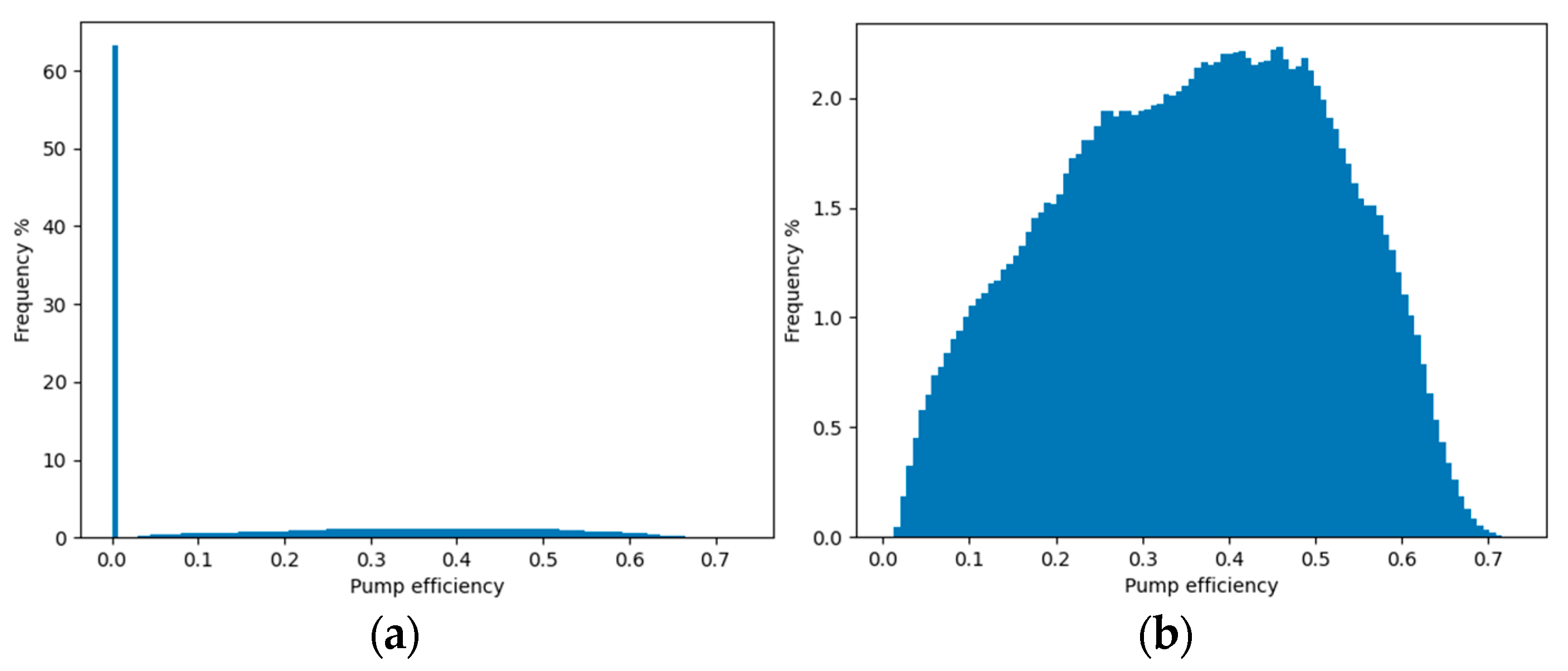
• Screening out data with a pump efficiency of 0:

Since the parameters were randomly generated, in most cases, most of the tapered pump combinations did not meet the production requirements, resulting in a pump efficiency of 0 for most calculation cases. This type of data constitutes a large proportion and, if retained, would negatively affect the model’s accuracy. Moreover, low pump efficiency combinations have little reference value for the final selection. Therefore, before training, these cases were excluded. After the screening, 3,659,452 valid data points remained. The pump efficiency distribution histogram before and after screening is shown in Figure 3.

• Screening out data with an operating frequency greater than 99 Hz:

During the calculation process, there may be instances where, due to small ESP models or levels, even if the operating frequency reaches the set upper limit, the ESP head still cannot meet the required lifting conditions. In such cases, an operating frequency is calculated, but this has no practical significance. This part of the data was also screened out. After this screening, 3,653,647 valid data points remained.

• Parameter normalization:

Normalization is the process of scaling the original data within a fixed range [0–1] to eliminate the impact of differences in the order of magnitude between various parameters and reduce analysis errors. This process is performed for both input and output parameters. The normalization function is as follows:

$$x^{*}={\displaystyle \frac{x-min\left(x\right)}{max\left(x\right)-min\left(x\right)}}$$

(4)

Additionally, since the overall pump efficiency is the most important output parameter in the model, it was normalized and multiplied by a factor of 1.2 to amplify its contribution to the error during training, thereby improving the accuracy of the calculations.

• Data set division:

After preprocessing, the dataset was divided into a training set, validation set, and test set in the following proportions: 70%, 15%, and 15%, respectively.

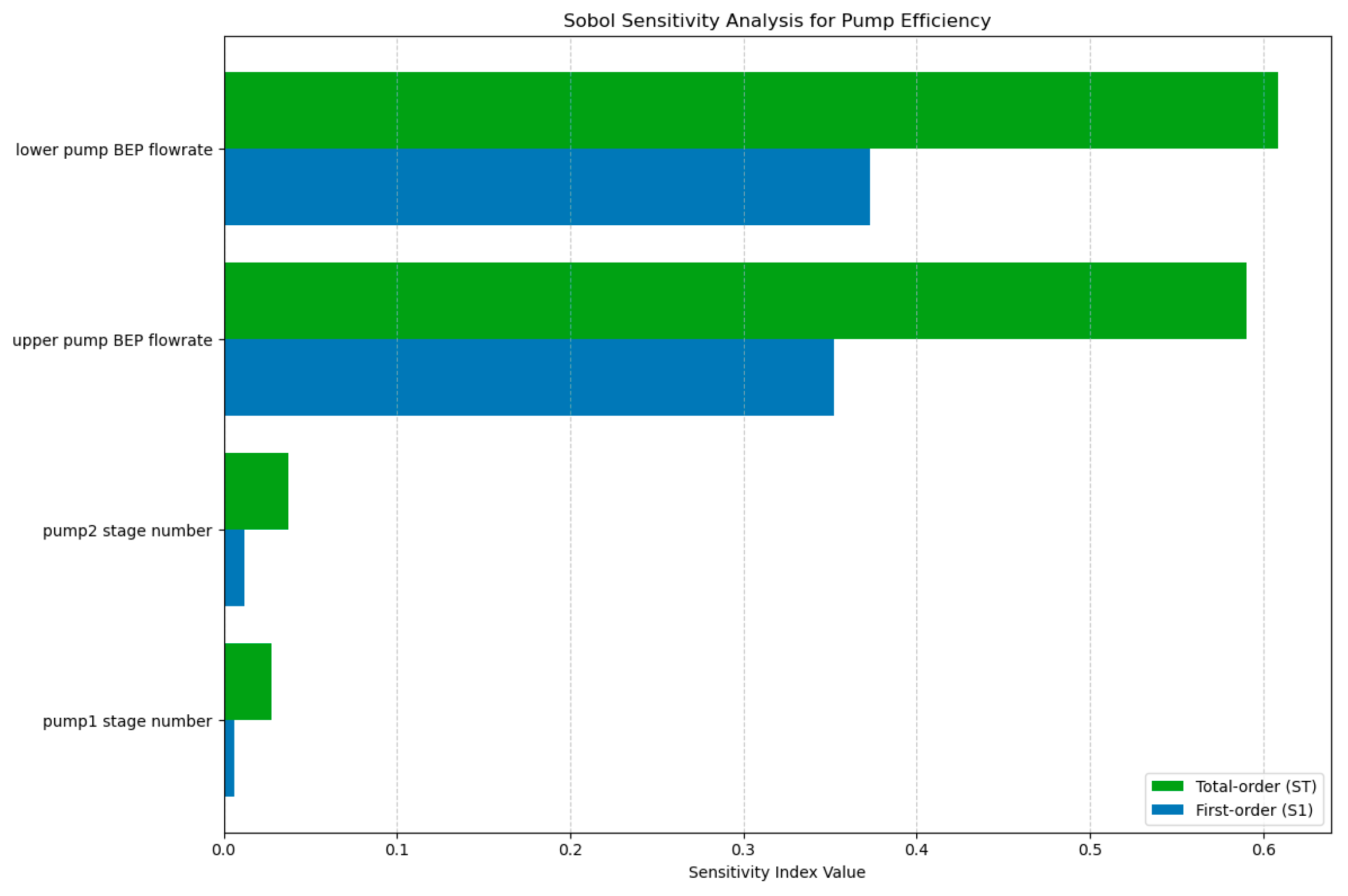
• Sensitivity analysis of input parameters:

To identify the most influential pump sizing parameters on pump efficiency, a sensitivity analysis was conducted using the Sobol method. Given the complexity of the ESP performance curves, the best efficiency point (BEP) flow rate of each pump model was used to represent the pump characteristics. The results of the sensitivity analysis are shown in Figure 4. The analysis reveals that the BEP flow rates (pump models) of two pumps are the most significant factors affecting pump efficiency, accounting for approximately 60% of the total variance. In contrast, the pump stage numbers have a relatively minor impact. This finding underscores the importance of selecting pumps with appropriate BEP flow rates to maximize efficiency while the number of stages can be adjusted within a reasonable range without significantly affecting performance.

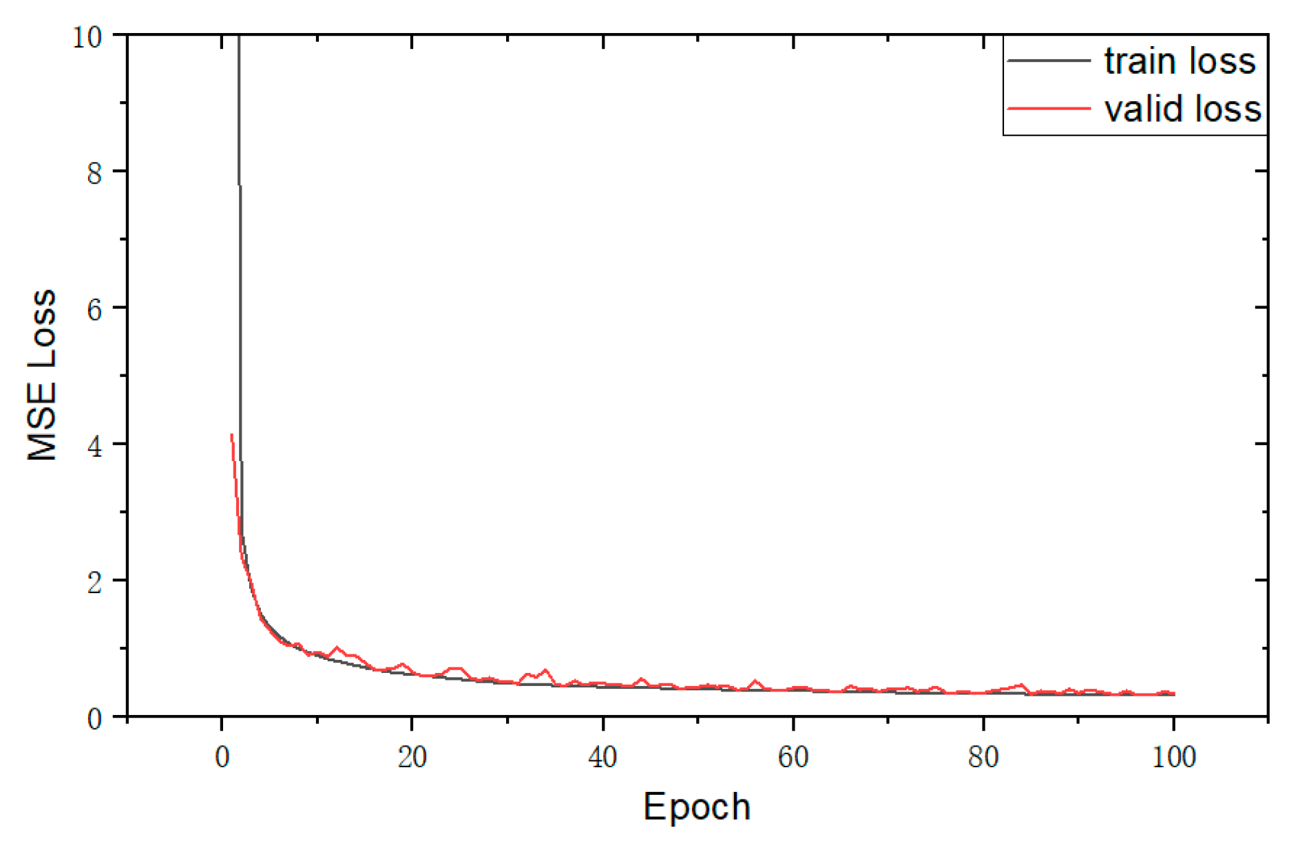
3.3. Model Building and Training

The FCNN model was trained on a PC equipped with an Intel i7-14700K CPU (Intel Corporation, Santa Clara, CA, USA, 20 cores, 5.6 GHz) and 32 GB RAM, utilizing PyTorch 2.5.1 in CPU-only mode. To determine the optimal architecture for the fully connected neural network (FCNN), we evaluated several configurations with varying numbers of hidden layers and neurons. The performance metrics and training times for each configuration are summarized in

Table 2. Performance comparison of different neural network architectures.

Network Architecture *	Training Time (s)	Test MAE	Test MSE	Test R2
33-16-8	1714.06	2.6474	16.7345	0.9569
33-64-8	1952.41	1.1303	3.2766	0.9910
33-64-32-8	2672.63	0.6147	0.9529	0.9974
33-64-32-16-8	2716.26	0.6151	0.9172	0.9974
33-128-64-32-8	2811.20	0.3431	0.3231	0.9991
33-128-64-32-16-8	3327.19	0.3168	0.2610	0.9993

* The notation “X-Y-Z-…” represents the number of neurons in each layer, where X is the input layer, Y, Z, … are hidden layers, and the last number is the output layer.

. The mean absolute error (MAE), the mean squared error (MSE), and the coefficient of determination (R²) were used to evaluate the accuracy of the FCNN model.

The results show that architecture 33-128-64-32-8 achieved the best balance between prediction accuracy and computational efficiency. While the more complex architecture achieved slightly better performance, its training time was significantly longer. On the other hand, simpler architectures exhibited higher prediction errors despite their shorter training times. So, the network architecture used in this model consists of five fully connected layers. The input layer contains 33 neurons, corresponding to 33 input features. The three hidden layers contain 128, 64, and 32 neurons, respectively. The output layer consists of eight neurons, each corresponding to a target variable. The input and output parameters are shown in

Table 3. Input and output parameters for FCNN model.

Network Layer	Parameters	Number of Neurons
Input layer	Intake pressure	1
	Discharge pressure	1
	Liquid production rate	1
	Tubing GLR	1
	Fluid temperature	1
	Water relative density	1
	Water relative density	1
	Head curve of lower pump	6
	Efficiency curve of lower pump	6
	Stage number of lower pump	1
	Head curve of upper pump	6
	Efficiency curve of upper pump	6
	Stage number of upper pump	1
Output layer	Operating frequency	1
	Total pump efficiency	1
	Flow rate at intake/discharge/connection point	3
	GVF at intake/discharge/connection point	3

.

During the training process, the mean squared error (MSE) was used to define the loss function during the training process. To enhance the model’s accuracy, we conducted extensive experiments to fine-tune the hyperparameters, including the learning rate, batch size, and number of epochs. The optimal combination was found to be a learning rate of 0.001 and a batch size of 128, which resulted in the lowest loss for the validation dataset. Additionally, we employed the rectified linear unit (ReLU) activation function for all hidden layers to introduce nonlinearity while avoiding the vanishing gradient problem. We experimented with different combinations of batch size and learning rate. The optimal combination was found to be a batch size of 128 and a learning rate of 0.001, which resulted in the lowest loss for the test data set. To ensure the robustness and generalizability of the proposed model, several measures were implemented during the data generation and model training phases. First, the input parameters for the training data were randomly generated within specified ranges, and a large-scale dataset was created to minimize the risk of overfitting. Second, L2 regularization with a coefficient of 0.0001 was incorporated into the loss function during model training to control the complexity of the neural network and prevent overfitting. Finally, to rigorously evaluate the model’s stability and generalization ability, a 5-fold cross-validation was performed. The results showed consistent performance across all folds, with an average MSE of 0.3538 for the training set and 0.3905 for the validation set, indicating the model’s high reliability and robustness. The train loss and valid loss for each epoch are shown in Figure 5.

Minor discrepancies can be attributed to the nonlinear behavior of multiphase flow under such scenarios. However, these errors are within acceptable limits for engineering applications, and the overall performance of the FCNN model is deemed satisfactory. A comparison of the operating frequency, flow rate, GVF, and pump efficiency, as calculated by the mechanism model and the FCNN model, is presented in Figure 6.

Additionally, based on this comparison, under the same hardware configuration, the mechanism model took 62.57 s to calculate 1000 data points, whereas the FCNN model only required 2.58 s to calculate 2,300,000 data points, significantly increasing the calculation speed.

4. Case Study and Validation

4.1. Case Description

As an example, consider an actual dewatering gas well. The basic information for the well is shown in

Table 4. D1 well data.

Data	Value	Data	Value
Well structure	Vertical	Tubing ID (mm)	63
Water relative density	1.02	Casing ID (mm)	121
Gas specific gravity	0.66	Pump fluid temperature (K)	353
Perforation depth (m)	3200	Pump hanging depth (m)	3000
Gas separator efficiency	0.9

.

The production characteristics of the gas reservoir vary across different stages. During the initial production stage, the system is in a strong dewatering stage, characterized by a high liquid production rate. In the middle stage, as the bottom hole pressure decreases, gas production increases while water production declines. In the late stage, liquid production continues to decrease, and gas production remains at a high level. The production parameters of the gas well under three typical operating conditions are provided in

Table 5. Operating parameters of Well D1 under three typical cycles.

Working Condition Name	Gas Rate (m3/d)	Water Rate (m3/d)	Intake Pressure (MPa)	Discharge Pressure (MPa)	Tubing GLR (m3/m3)	Weight Coefficients
1	20,000	200	17.90	28.04	10	0.25
2	30,000	100	13.21	24.72	30	0.25
3	30,000	50	8.3	22.15	60	0.5

. The intake and discharge pressure are determined using the Beggs–Brill wellbore two-phase flow calculation model, with the bottom hole flowing pressure and wellhead tubing pressure serving as the starting points, respectively. When calculating the weighted pump efficiency, working condition 3 has the longest duration, so the weight coefficients for the three working conditions are set as 0.25, 0.25, and 0.5, respectively.

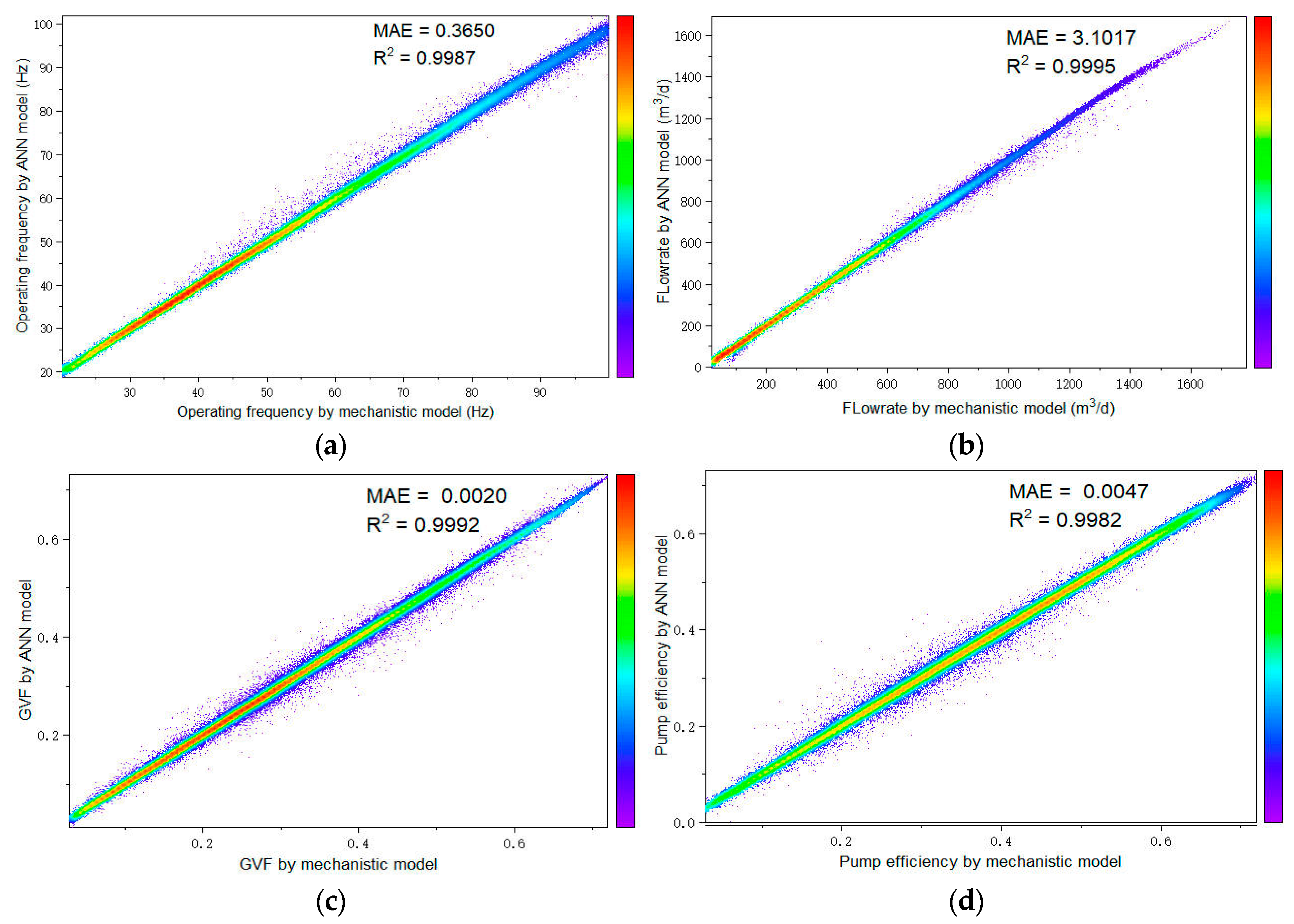
4.2. FCNN Model Calculation Results

Based on the parameters outlined above and using the parameters from the ESP database, the operating parameters of tapered ESP with each pump model and stage number combination are calculated using the FCNN model. After applying the ESP sizing empirical model to screen out invalid combinations, a total of 10,901 pump model and stage number combinations are retained. Among these, the tapered pump combination with the highest weighted pump efficiency consists of a 74-stage G12 and a 92-stage P10, and the weighted efficiency is 43.36%. The operating parameters for this combination under various working conditions are shown in

Table 6. Operating parameters of 74-G12 and 92-P10 tapered pumps under three typical working conditions.

Working Condition	Operating Frequency (Hz)	Intake Flow Rate (m3/d)	Connection Point Flow Rate (m3/d)	Discharge Flow Rate (m3/d)	Intake GVF	Connection Point GVF	Discharge GVF	Pump Efficiency (%)
1	56.8	215.62	206.97	211.49	0.0494	0.0481	0.0422	45.37
2	51.3	124.02	114.06	112.11	0.1830	0.1396	0.1138	59.53
3	59.5	87.39	68.08	65.50	0.4292	0.2991	0.2138	38.31

.

Additionally, the pump efficiency and operating frequency for several sets of ESP models and series combinations, ranked by weighted pump efficiency, are displayed in

Table 7. Operation parameters of several tapered pump models and stage number combinations with higher weighted pump efficiency.

Lower Pump	Upper Pump	Condition 1		Condition 2		Condition 3		Weighted Pump Efficiency
		Operating Frequency (Hz)	Pump Efficiency	Operating Frequency (Hz)	Pump Efficiency	Operating Frequency (Hz)	Pump Efficiency
74-G12	92-P10	56.8	45.37%	51.3	51.45%	59.5	38.31%	43.36%
100-G22	128-P18	49.1	62.90%	50.9	47.10%	59.2	30.37%	42.69%
74-G12	96-P8	60.5	38.95%	51.4	51.55%	59.2	39.45%	42.35%
76-G12	96-P12	52.5	50.84%	50.4	49.79%	59.5	34.01%	42.16%
98-G22	98-P12	50.7	54.30%	49.5	48.58%	59.2	32.33%	41.88%
98-G22	92-P10	55.7	45.86%	50.4	49.79%	59.4	35.44%	41.63%
98-G22	94-P8	59.4	40.22%	51.8	49.02%	59.5	36.27%	40.44%

. The combinations with the same pump model and similar stage numbers have been screened out. The selected pump models belong to the same series and can be used as tapered ESP systems.

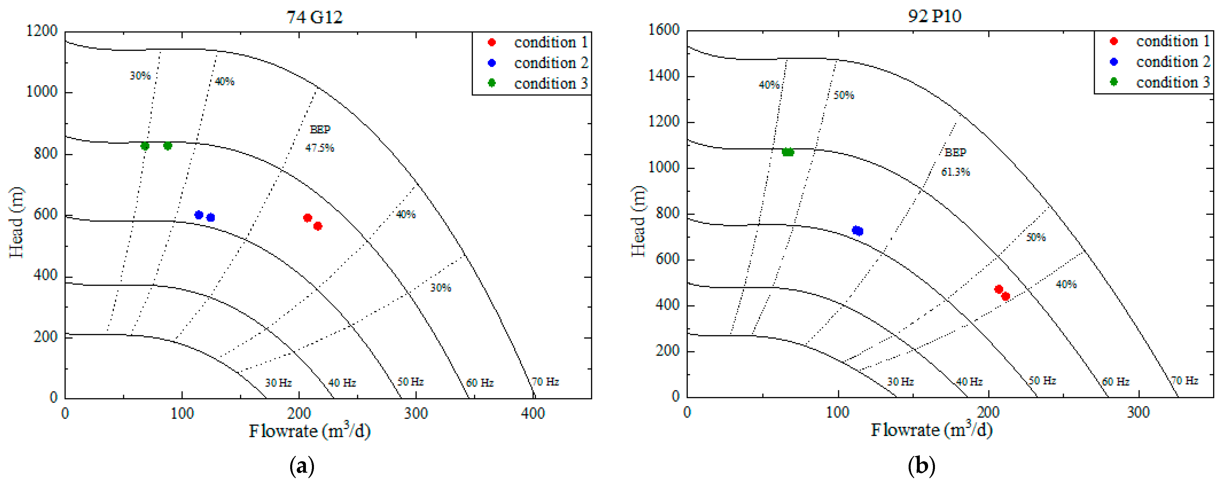
4.3. Sizing Results Analysis

The working points of 74-G12 and 92-P10 under various preset working conditions are plotted on the ESP performance tornado curves, as shown in Figure 7. The dotted lines in the figure represent the working points corresponding to the same pump efficiency at different operating frequencies. Each pump has two points under each working condition, representing the working points corresponding to the intake and discharge parameters of each pump. As can be analyzed from Figure 7, all operating points are located in the range of higher pump efficiency, thus ensuring the efficient operation of the pump and reducing the potential risk of failure.

5. Conclusions

This study developed a sizing model for tapered ESP systems, which accurately predicts various operating parameters under multiple working conditions. The key contributions and findings of this research include the following: The proposed FCNN model demonstrates exceptional prediction accuracy, with an MAE of 0.3431, an MSE of 0.3231, and an R² of 0.9991. This significantly outperforms traditional empirical formulas and simplified models. By integrating the FCNN model with conventional models, such as the wellbore two-phase flow model and ESP sizing empirical rules, the hybrid model achieves a significant improvement in computational efficiency, reducing calculation time while maintaining high accuracy. The model automates the selection of optimal pump configurations, including pump models and stage numbers, under multiple operating conditions; this ensures maximum pump efficiency and minimizes the risk of operational failures. While the proposed model has shown promising results, several areas warrant further investigation to enhance its applicability and impact. Future research could explore the applicability of the model to other types of pumps, such as progressive cavity pumps. Developing a real-time version of the model could enable dynamic adjustment of pump parameters during operation, further improving efficiency and adaptability. Incorporating IoT sensors and big data analytics could provide more accurate input data and enhance the model’s predictive capabilities, particularly in complex and dynamic well conditions. These future directions aim to further enhance the model’s applicability and impact, paving the way for broader adoption in both academic research and industrial applications.

References

1. Janadeleh, M.; Ghamarpoor, R.; Abbood, N.K.; Seyednooroldin, H.; Hasan, N.; Ali, Z.H. Evaluation and selection of the best artificial lift method for optimal production using pipesim software. Heliyon 2024, 10, e36934. [Google Scholar] [CrossRef] [PubMed]
2. Drozdov, A.N.; Bulatov, G.G.; Lapoukhov, A.N.; Mamedov, E.A.; Malyavko, E.A.; Alekseev, Y.L. Artificial-lift operation technologies of low-pressure flooded gas and gas-condensate wells. In Proceedings of the SPE Trinidad and Tobago Section Energy Resources Conference, Port-of-Spain, Trinidad, 11 June 2012. [Google Scholar] [CrossRef]
3. Pant, H. Best Pumping Practices to Optimize Dewatering in CBM wells: Lessons Learned Developing Raniganj East Field, India. In Proceedings of the SPE Unconventional Resources Conference and Exhibition-Asia Pacific, Brisbane, Australia, 11 November 2013. [Google Scholar] [CrossRef]
4. Bassett, L. Successful Strategies for Dewatering Wells Using ESP’s. In Proceedings of the SPE Eastern Regional Meeting, Charleston, SC, USA, 23 September 2009. [Google Scholar] [CrossRef]
5. Liang, X.; Xing, Z.; Yue, Z.; Ma, H.; Shu, J.; Han, G. Optimization of Energy Consumption in Oil Fields Using Data Analysis. Processes 2024, 12, 1090. [Google Scholar] [CrossRef]
6. Buluttekin, M.B.; Ulusoy, B.; Dorscher, D. Simulations and challenges of ESP applications in high GOR wells at south east of Turkey. In Proceedings of the 22nd World Petroleum Congress, Istanbul, Turkey, 9 July 2017. [Google Scholar]
7. Zhou, D.; Sachdeva, R. Design Tapered Electric Submersible Pumps For Gassy Wells. In Proceedings of the Indian Oil and Gas Technical Conference and Exhibition, Mumbai, India, 4 March 2008. [Google Scholar] [CrossRef]
8. Peng, Y.; Ye, C.; Sun, F.; Wang, X.; Zhu, P.; Zhu, Q.; Zhang, Y.; Wang, W. Drainage gas recovery technology for high-sulfur gas wells by a canned ESP system. Nat. Gas Ind. B 2018, 5, 452–458. [Google Scholar] [CrossRef]
9. Kadio-Morokro, B.; Curay, F.; Fernandez, J.; Salazar, V. Extending ESP run life in gassy wells application. In Proceedings of the SPE Electric Submersible Pump Symposium, The Woodlands, TX, USA, 24 April 2017. [Google Scholar] [CrossRef]
10. Takacs, G. Electrical Submersible Pump Components and Their Operational Features. In Electrical Submersible Pumps Manual, 2nd ed.; Gulf Professional Publishing: Waltham, MA, USA, 2018; pp. 55–152. [Google Scholar] [CrossRef]
11. Yao, J.; Han, G.; Zhang, Z. Method of Automatic Sizing and Selection of Tapered Electrical Submersible Pump System Based on Multiple Operating Cases. In Proceedings of the International Conference on Computational & Experimental Engineering and Sciences, Singapore, 21 August 2024. [Google Scholar] [CrossRef]
12. Agwu, O.E.; Alkouh, A.; Alatefi, S.; Azim, R.A.; Ferhadi, R. Utilization of machine learning for the estimation of production rates in wells operated by electrical submersible pumps. J. Pet. Explor. Prod. Technol. 2024, 14, 1205–1233. [Google Scholar] [CrossRef]
13. Yang, P.; Chen, J.; Wu, L.; Li, S. Fault Identification of Electric Submersible Pumps Based on Unsupervised and Multi-Source Transfer Learning Integration. Sustainability 2022, 14, 9870. [Google Scholar] [CrossRef]
14. Peng, L.; Han, G.; Pagou, A.L.; Shu, J. Electric submersible pump broken shaft fault diagnosis based on principal component analysis. J. Pet. Sci. Eng. 2020, 191, 107154. [Google Scholar] [CrossRef]
15. Wan, M.; Gou, M. Research on fault diagnosis of electric submersible pump based on improved convolutional neural network with Bayesian optimization. Rev. Sci. Instrum. 2023, 94, 115109. [Google Scholar] [CrossRef] [PubMed]
16. Han, G.; Lu, X.; Zhang, H.; Sui, X.; Wang, B.; Liang, K. ESP Wells Dynamic Survival Analysis and Lifespan Prediction Using Machine Learning Algorithms. In Proceedings of the SPE Annual Technical Conference and Exhibition, New Orleans, LA, USA, 20 September 2024. [Google Scholar] [CrossRef]
17. Abdalla, R.; Samara, H.; Perozo, N.; Carvajal, C.P. Machine learning approach for predictive maintenance of the electrical submersible pumps (ESPS). ACS Omega 2022, 7, 17641–17651. [Google Scholar] [CrossRef] [PubMed]
18. Costa, E.A.; Rebello, C.M.; Santana, V.V.; Reges, G.; Silva, T.O.; Abreu, O.S.L.; Ribeiro, M.P.; Foresti, B.P.; Fontana, M.; Nogueira, I.B.R.; et al. An uncertainty approach for Electric Submersible Pump modeling through Deep Neural Network. Heliyon 2024, 10, e24047. [Google Scholar] [CrossRef]
19. Iranzi, J.; Son, H.; Lee, Y.; Wang, J. A Nodal Analysis Based Monitoring of an Electric Submersible Pump Operation in Multiphase Flow. Appl. Sci. 2022, 12, 2825. [Google Scholar] [CrossRef]
20. Beggs, D.H.; Brill, J.P. A study of two-phase flow in inclined pipes. J. Pet. Technol. 1973, 25, 607–617. [Google Scholar] [CrossRef]
21. Heidaryan, E.; Salarabad, A.; Moghadasi, J. A novel correlation approach for prediction of natural gas compressibility factor. J. Nat. Gas Chem. 2010, 19, 189–192. [Google Scholar] [CrossRef]
22. Bahadori, A.; Mokhatab, S.; Towler, B.F. Rapidly estimating natural gas compressibility factor. J. Nat. Gas Chem. 2007, 16, 349–353. [Google Scholar] [CrossRef]
23. Hall, K.R.; Yaborough, L. A new equation of state for Z-factor calculations. Oil Gas J. 1973, 71, 82–92. [Google Scholar]
24. Zhu, J.; Zhu, H.; Wang, Z.; Zhang, J.; Cuamatzi-Melendez, R.; Farfan, J.A.M.; Zhang, H.Q. Surfactant effect on air/water flow in a multistage electrical submersible pump (ESP). Exp. Therm. Fluid. Sci. 2018, 98, 95–111. [Google Scholar] [CrossRef]
25. Ali, A.; Yuan, J.; Deng, F.; Wang, B.; Liu, L.; Si, Q.; Buttar, N.A. Research Progress and Prospects of Multi-Stage Centrifugal Pump Capability for Handling Gas–Liquid Multiphase Flow: Comparison and Empirical Model Validation. Energies 2021, 14, 896. [Google Scholar] [CrossRef]
26. Zhu, J.; Zhang, H.-Q. A Review of Experiments and Modeling of Gas-Liquid Flow in Electrical Submersible Pumps. Energies 2018, 11, 180. [Google Scholar] [CrossRef]
27. Andagoya, K.; Villalobos, J.; León, F.; Hidalgo, M.; Vela, N.; Sotomayor, A.; Orozco, A.; Ekambaram, R.; Koduru, P.; Reyes, C.; et al. Ultrahigh Speed ESP Technology Solution for a 11,400-ft Well: First Successful Deployment with Induction Motor in Ecuador. In Proceedings of the SPE Middle East Artificial Lift Conference and Exhibition, Manama, Bahrain, 29 October 2024. [Google Scholar] [CrossRef]
28. Powers, M.L. Special considerations for electric submersible pump applications in underpressured reservoirs. SPE Prod. Eng. 1992, 7, 301–306. [Google Scholar] [CrossRef]
Figure 1. Schematic diagram of a tapered ESP system.
Processes 13 01056 g001
Figure 2. Schematic diagram of the structure of the hybrid model for tapered ESP sizing based on multiple working conditions.
Processes 13 01056 g002
Figure 3. Pump efficiency distribution histogram before and after screening out data with a pump efficiency of 0: (a) before screening; (b) after screening.
Processes 13 01056 g003
Figure 4. Sensitivity analysis of sizing parameters on efficiency using Sobol method.
Processes 13 01056 g004
Figure 5. Model training loss convergence curve.
Processes 13 01056 g005
Figure 6. Comparison of calculation results of mechanism model and FCNN model: (a) operating frequency; (b) flow rate; (c) GVF; and (d) pump efficiency.
Processes 13 01056 g006
Figure 7. Pump tornado curves and operating points of each operating condition: (a) 74-G12 and (b) 92-P10.
Processes 13 01056 g007