The Influence of Parabolic Static Mixers on the Mixing Performance of Heavy Oil Dilution

Abstract

The static mixer is one of the key equipment for dilution transportation of heavy oil. To enhance the mixing performance of heavy oil dilution, a static mixer featuring a parabolic blade has been developed through an innovative redesign of the traditional Kenics blade. Numerical simulations of the parabolic static mixer were conducted using Fluent 2022 R1 software. The coefficients of concentration variation (COV) and pressure drop (∆P) served as evaluation indexes, and the effects of parabolic focal length (P), torsion angle (α), and length–diameter ratio (Ar) of the mixing blade on mixing performance were thoroughly analyzed. The research indicates that setting the mixing blade parameters to P = 60, α = 180°, and Ar = 1.5 results in improved mixing performance compared to the traditional Kenics static mixer, achieving a COV of 0.036, which signifies nearly complete mixing of heavy oil and light oil. As parabolic P increases, ∆P exhibits a decreasing trend, while the COV begins to show a significant difference at the outlet of the third mixing blade. As α increases, ∆P rises, while the COV decreases. A decrease in Ar causes ∆P to increase sharply. Although heavy oil and light oil can mix rapidly over a short distance, their influence on the final mixing effect is relatively minor. This study offers significant theoretical insights and practical implications for high-efficiency heavy oil dilution transportation technology.

1. Introduction

The dilution transportation of heavy oil has become prevalent in the current pipeline industry [1,2]. Due to its high viscosity, density, and poor fluidity, heavy oil cannot mix efficiently with light oil [3,4,5]. Therefore, it is essential to disrupt the structural flow characteristics of heavy oil and light oil through the rotation, stretching, and segmentation of mixing components to enhance the mixing effect [6].

Mixers can be categorized into dynamic and static types based on their mixing methods. Researchers both locally and globally have conducted extensive studies on the performance of various types of mixers. Liu Chengwen et al. [7] investigated the impact of down-hole swirl mixers on the mixing effect of light and heavy oils through numerical simulations. Their findings indicated that down-hole mixers significantly enhance the mixing uniformity of light and heavy oils, effectively improving viscosity reduction effect [7]. Xiao Fei and Wang Xu et al. further explored the impact of static mixers on the distribution of the mixing flow field and the mixing effectiveness in down-hole risers [8,9]. Li Qin et al. proposed a novel dynamic mixer that outperforms traditional mixers in the dilution mixing of heavy oil [10]. Shi Chunwei et al. studied the influence of an ultrasonic static mixer on viscosity reduction of heavy oil, determined the best process parameters, calculated energy consumption during ultrasonic treatment and crushing, and measured the maximum viscosity reduction rate of 57.34% [11]. Zhang Yuan and colleagues designed a new core-tube mixer for heavy oil dilution that achieves efficient mixing through microhole injection and a variable-section cone design [12]. Liang Zheng et al., based on the Fluent transient numerical simulation method of pressure boundary, studied the real situation of light heavy oil mixing in the well, revealed the root cause of the slug condition of wellhead oil output, and proposed a quantitative dilution method [13]. Wan Jie et al. ameliorated the problem of uneven water distribution during water-containing heavy oil transportation by introducing a Kenics static mixer. Fluent software was used to simulate the flow field in the pipeline, and the homogenization effect was evaluated by the coefficient of variation and average droplet particle size. It was found that the Kenics static mixer could effectively homogenize the two phases of oil and water and reduce droplet particle size [14]. Rahimi et al. investigated the effect of agitator positioning on the homogenization time of crude oil storage tanks, finding that mixing efficiency was maximized when the agitator was located in the bottom quarter of the tank [15].

Mixers can be categorized into dynamic and static types based on their mixing methods. Wang Zongyong et al. simulated the breakup and coalescing behavior of oil droplets in a Kenics static mixer by using the CFD–PBM coupling method. The influence of the Reynolds number, number of mixed elements, and ratio of component length to diameter on the particle size of dispersed-phase droplets is analyzed. The results show that an increase in the Reynolds number leads to a decrease in the particle size at the exit of dispersed-phase droplets and the droplet size decreases rapidly in the first several component segments. The smaller the component length-to-diameter ratio is, the smaller the droplet exit particle size is [16]. Zhang Chunmei et al. proposed a new three-helix static mixer. Fluent software was used to perform numerical simulation analysis on static mixers with five different rotational element arrangement angles at a low Reynolds number. The research showed that the smaller the angle was, the better the mixing effect was, and the energy consumption decreased with the increase of the angle [17]. Tang Yang et al. designed a perforated Kenics static mixer and studied the influences of the perforation inner diameter, perforation spacing, and mixing unit length-to-diameter ratio on mixing performance. The results show that the perforation structure can significantly change the fluid flow state and improve mixing effect [18]. Meng Lichang et al. designed a rotary punch static mixer (RPSM), experimentally analyzed the effects of the installation mode, clearance, angle, and other parameters on the pressure drop, and established an empirical model of the Z factor. The results show that the reverse installation pressure drop is high and the pressure drop increases with the increase of the gap. The calculation of the Z factor is consistent with the experimental value [19]. Maoyun et al. introduced a novel spiral jet mixer and identified key parameters through CFD calculations to enhance the viscosity reduction of heavy oil [20]. Although dynamic mixers are capable of achieving uniform mixing, they require external drive systems, resulting in high energy consumption and substantial maintenance costs. In contrast, static mixers, which have no moving parts and utilize the fluid’s inherent kinetic energy for mixing, offer significantly lower energy consumption. However, traditional static mixers, such as the Kenics type, are inadequate for meeting the specific demands of heavy oil dilution transportation.

Currently, research on heavy oil dilution primarily focuses on down-hole dilution lifting and storage tank mixing, with most mixers being dynamic or ejector types. However, studies on the mixing performance of static mixers for the dilutive transport of heavy oil are relatively limited. To address this gap, this paper presents an innovative static mixer with a parabolic blade, building on the traditional Kenics design. Using heavy oil and light oil as the study subjects, this research analyzes the effects of the parabolic static mixer on the mixing performance of heavy oil under varying focal lengths (P), torsion angles (α), and length–diameter ratios (Ar) using Fluent software. The coefficients of concentration variation (COV) and pressure drop (∆P) serve as evaluation indexes for quantitatively analyzing these effects and trends, providing a theoretical reference for high-efficiency heavy oil dilution transport technology.

2. Materials and Methods

2.1. Description of the Equipment

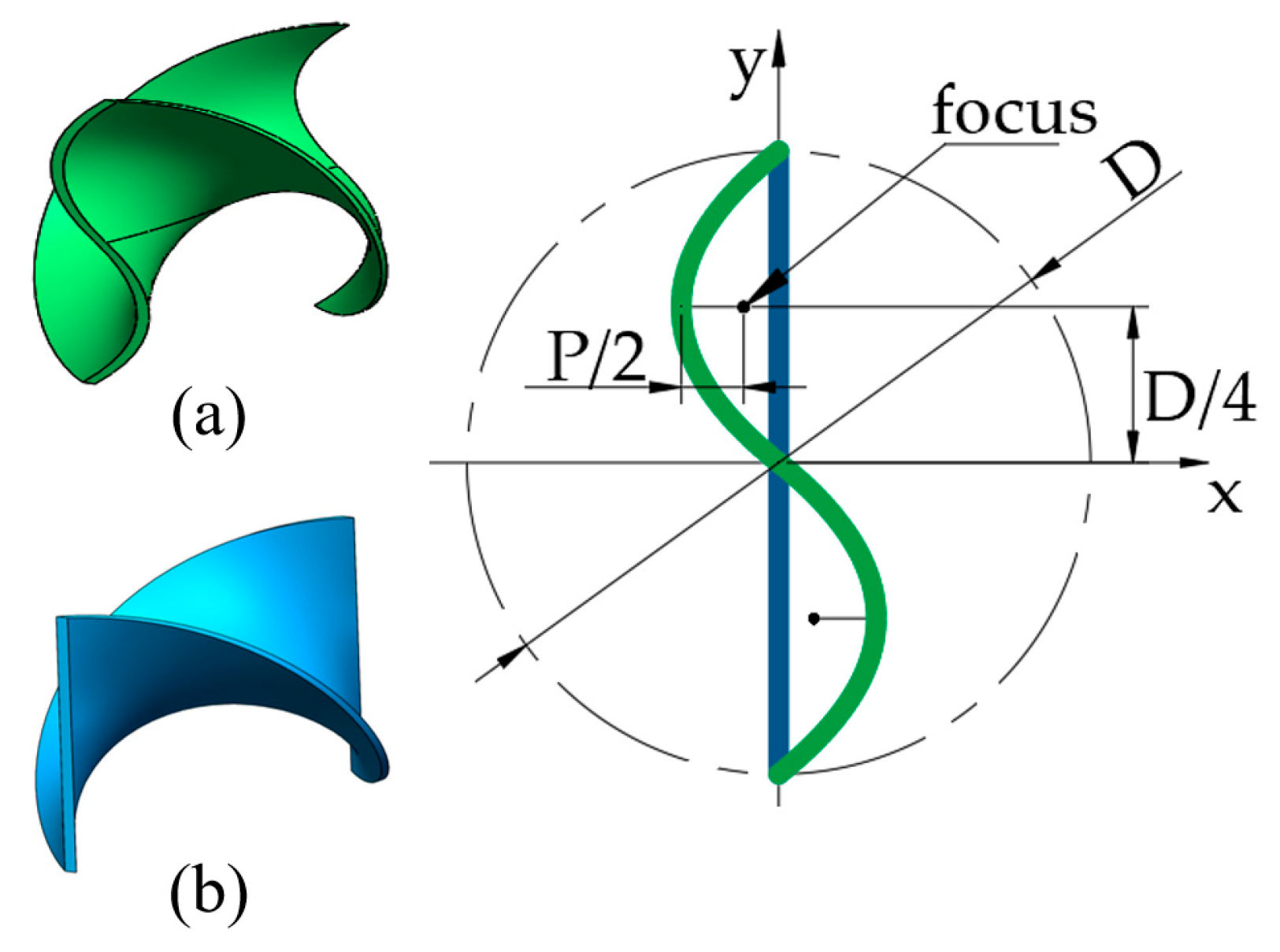
2.1.1. Design of the Parabolic Mixing Blade

Utilizing the conic curve theory proposed by Apollonius, a parabolic blade cross-section curve is developed to replace the traditional Kenics blade cross-section curve.

The parabola formula is as follows:

$$\left\{\begin{array}{ll}x={\displaystyle \frac{y^2}{2\mathrm{P}}}-{\displaystyle \frac{\mathrm{D}y}{4\mathrm{P}}}& \hfill (0<y\le {\displaystyle \frac{\mathrm{D}}{2}})\hfill \\ x=0& \hfill (y=0)\hfill \\ x=-{\displaystyle \frac{y^2}{2\mathrm{P}}}-{\displaystyle \frac{\mathrm{D}y}{4\mathrm{P}}}& \hfill (-{\displaystyle \frac{\mathrm{D}}{2}}\ge y<0)\hfill \end{array}\right.$$

(1)

where D is the torsional diameter of the mixing blade helix and P is the focal length of a parabola.

Subsequently, the three-dimensional structure of the mixing blade is generated using helical scanning technology, with its structural parameters illustrated in Figure 1. In the design of the parabolic blade, the vertical distance from the parabolic focus to the coordinate origin is D/4, while the distance from the paraboloid focus to the vertex is half the focal distance, P/2. It is observed that as P increases, the opening width of the parabola correspondingly widens, while its curvature decreases.

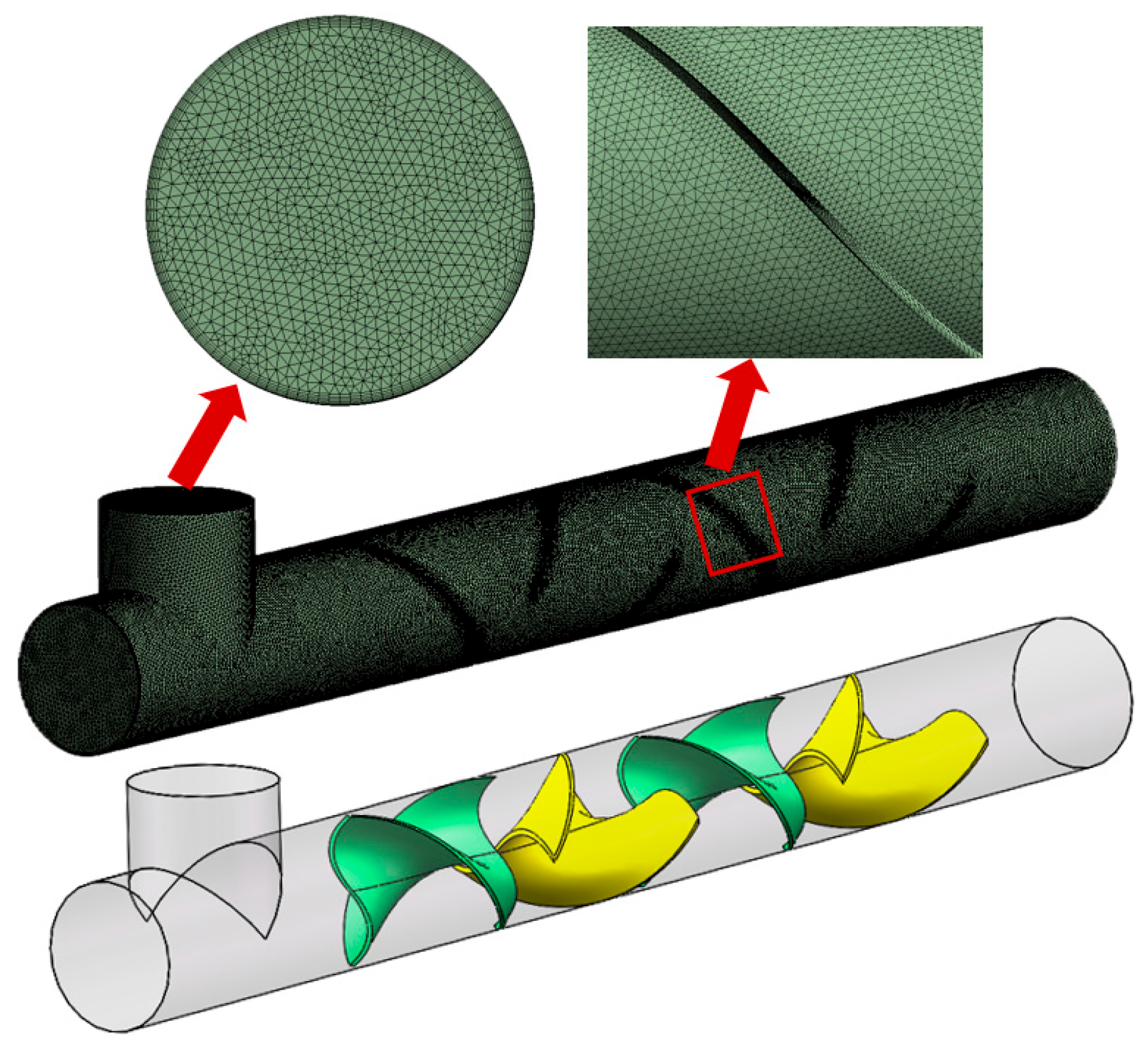
2.1.2. Geometric Model of Static Mixer

The pipeline for mixing and transporting heavy oil primarily consists of a main pipe for transporting heavy oil and a branch pipe for introducing light oil. A simplified model of the pipeline is created using SolidWorks 2019 3D modeling software, with four parabolic mixing blades installed inside, as illustrated in Figure 2. The angle between the inlet of heavy oil and light oil is 90°, the inner diameter of the mixing tube (D) is 50 mm, the length of the tube (L) is 500 mm, the length of the mixing blade (L1) is 75 mm, the distance from the heavy oil inlet to the first mixing blade (L2) is 125 mm, and the distance between the last mixing blade and the outlet (L3) is 75 mm. The distance between the centers of the heavy oil inlet and the light oil inlet (L4) is 50 mm. The distance from the light oil inlet to the pipe wall (L5) is 25 mm. The torsion angle of the mixing blade (α) is 180°, and the length-to-diameter ratio of the blade (Ar) is L1/D = 1.5. The left and right rotating blades are arranged alternately with a stagger of 90° within the tube. The thickness of the mixing blade (δ) is 2 mm, and the total length of the mixing blade area is 300 mm.

2.2. Evaluation Index

2.2.1. Mixing Effect

To quantitatively analyze the mixing effect of heavy oil dilution, this paper employs the coefficient of concentration variance (COV) [21] as an evaluation index. A smaller COV indicates a better two-phase mixing effect. When COV < 0.05, the two-phase fluids are considered to be nearly completely mixed. When 0.05 ≤ COV < 1, it indicates that the two-phase fluids are starting to mix. When COV = 1, it signifies that the two-phase fluids are in a state of complete separation.

The COV can be calculated by the following equation:

$$\mathrm{COV}={\displaystyle \frac{\sigma }{\overline{C}}}$$

(2)

$$\sigma =\sqrt{{\displaystyle \frac{1}{N}}{\displaystyle \sum _{i=1}^N{\left(C_i-\overline{C}\right)}^2}}$$

(3)

$$\overline{C}={\displaystyle \frac{1}{N}}{\displaystyle \sum _{i=1}^N{C}_i}$$

(4)

where $\overline{C}$ is the arithmetic average of the heavy oil volume fraction of the sampling section; C_i is the volume fraction of heavy oil at the i-sampling point of the sampling section; σ is the standard deviation; and N is the number of sampling points on the sampling section.

2.2.2. Pressure Drop

Pressure drop (∆p) is a crucial parameter for assessing the energy consumption associated with heavy oil dilution transportation. The calculation equation is as follows:

$$\Delta \mathrm{p} ={\mathrm{p}}_0-{\mathrm{p}}_1$$

(5)

where p₀ is the average pressure of the heavy oil inlet; p₁ is the average pressure of the sampling section.

2.3. Numerical Simulation

2.3.1. Continuity Equation and Momentum Equation

The Mixture model [22] was utilized to simulate the mixing effects of heavy oil and light oil. This model is a simplified multiphase flow framework designed to simulate two-phase or multiphase flow, allowing for the interpenetration of phases. It is particularly suitable for scenarios with a wide distribution of dispersed phases, offering low computational demands and high stability.

The continuity and momentum equations are as follows:

$${\displaystyle \frac{\partial }{\partial t}}\left({\rho }_m\right)+\nabla ·\left({\rho }_m{\overrightarrow{v}}_m\right)=0$$

(6)

$${\displaystyle \frac{\partial }{\partial \mathrm{t}}}\left({\rho }_m{\overrightarrow{v}}_m\right)+\nabla ·\left({\rho }_m{\overrightarrow{v}}_m·{\overrightarrow{v}}_m\right)=-\nabla p+\nabla ·\left[{\mu }_m\left(\nabla {\overrightarrow{v}}_m+\nabla {\overrightarrow{v}}_m^T\right)\right]+{\rho }_m{\overrightarrow{g}}_m+\overrightarrow{F}-\nabla ·\left({\displaystyle \sum _{k=1}^{\mathrm{n}}{\alpha }_k{\rho }_k{\overrightarrow{v}}_{dr,k}{\overrightarrow{v}}_{dr,k}}\right)$$

(7)

where ∇ is the Hamiltonian operator; ρ_m is the mixed density; ${\overrightarrow{v}}_m$ is the average mass velocity after mixing; μ_m is the dynamic viscosity after mixing; $\overrightarrow{F}$ is the volume force; α_k is the volume fraction of the secondary phase; and ${\overrightarrow{v}}_{dr,k}$ is the drift velocity of the secondary phase.

2.3.2. Turbulence Model

Since the mixed fluid generates a swirling flow field within the pipeline due to the mixing blades, the Realizable k-ε turbulence model is selected [23].

The turbulent kinetic energy equation and the dissipation rate transport equation are as follows:

$${\displaystyle \frac{\partial \left(\rho k\right)}{\partial t}}+{\displaystyle \frac{\partial \left(\rho k{u}_i\right)}{\partial x_j}}={\displaystyle \frac{\partial \left[\left(\mu +\frac{{\mu }_t}{{\sigma }_k}\right)\frac{\partial k}{\partial x_j}\right]}{\partial x_j}}+G_k+G_b-\rho \epsilon -Y_M+S_k$$

(8)

$${\displaystyle \frac{\partial \left(\rho \epsilon \right)}{\partial t}}+{\displaystyle \frac{\partial \left(\rho \epsilon u_j\right)}{\partial x_j}}={\displaystyle \frac{\partial \left[\left(\mu +\frac{{\mu }_t}{\sigma \epsilon }\right)\frac{\partial \epsilon }{\partial x_j}\right]}{\partial x_j}}+\rho C_1{S}_{\epsilon }-\rho C_2{\displaystyle \frac{{\epsilon }^2}{k+\sqrt{\nu \epsilon }}}+C_{1\epsilon }{\displaystyle \frac{\epsilon }{k}}{C}_{3\epsilon }{G}_b+S_{\epsilon }$$

(9)

where G_k is the generation term of turbulent kinetic energy k caused by the average velocity gradient; G_b is the generation term of turbulent kinetic energy k caused by buoyancy; Y_M is the compressibility correction term; C₁, C₂, C_1ε, and C_3ε are empirical constants; S_k and S_ε are the source terms of k and ε equations, respectively.

2.3.3. Boundary Conditions and Solving Methods

In this study, the primary phase fluid is heavy oil, while the secondary phase fluid is light oil. The physical property parameters of the fluids are presented in

Table 1. Fluid physical property parameters.

Fluid	Density/(kg/m3)	Viscosity/(Pa·s)
Heavy oil	950.1	4.488
Light oil	932.5	0.08421

. Both the primary and secondary phases utilize velocity inlets with a uniform velocity of 2.5 m/s, directed perpendicular to the inlet. The outlet employs a pressure outlet, with the reference pressure set to standard atmospheric pressure. The wall surface is fixed without slip conditions, and the turbulence characteristics at the inlet and outlet are defined using turbulence intensity and the hydraulic diameter.

The turbulent intensity and the hydraulic diameter are calculated as follows:

$$\mathrm{Re}={\displaystyle \frac{\rho vd}{\mu }}$$

(10)

$$I=0.16{\mathrm{Re}}^{-0.125}$$

(11)

$$D_H={\displaystyle \frac{4A}{C}}$$

(12)

where Re is the Reynolds number; ρ is fluid density; v is the fluid velocity; d is the diameter of the pipe; μ is fluid viscosity; I is turbulence intensity; A is the cross-sectional area of the inlet; C is the inlet perimeter; and D_H is the hydraulic diameter.

The density of liquids varies very little with pressure, and in most engineering applications, the change in density is negligible. In long-distance oil pipelines, the pressure difference provided by the pumping station can reach tens to hundreds of atmospheres, and the static pressure change caused by gravity is relatively small. In addition, the static mixer studied in this paper has small geometric size, and the influence of gravity is much less than other forces at this scale. In this study, the following assumptions are made regarding the two-phase fluids: both fluids are treated as incompressible Newtonian fluids, and the influence of gravity is neglected in the numerical simulation. The SIMPLE algorithm is employed for coupling pressure and velocity, while the First-Order Upwind scheme is applied to the spatial discretization of the equations. The residual for the continuous phase equation is set to 1 × 10⁻⁵, while the residual for the other equations is set to 1 × 10⁻⁶.

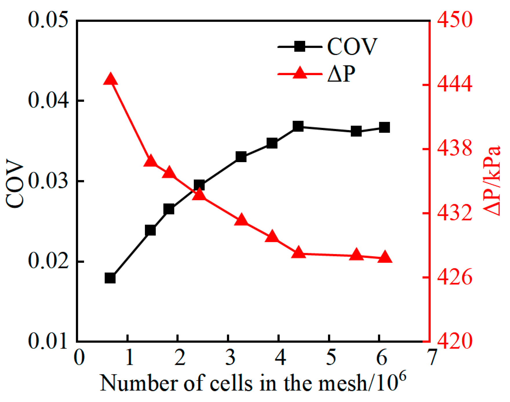
2.3.4. Mesh Independence Verification

Meshing can significantly impact the experimental results of numerical simulations. An excessively high mesh density can compromise computational efficiency and increase costs, whereas an excessively low mesh density may affect computational accuracy. Therefore, it is essential to select an appropriate mesh density for numerical simulations. The parabolic static mixer with structural parameters of P = 60 mm, α = 180°, and Ar = 1.5 was meshed using Fluent 2022 R1 software. The entire model was discretized using tetrahedral meshes, with the blade surfaces set as walls. The maximum number of wall layers was set to 5, with a growth rate of 1.2, as illustrated in Figure 3. The COV and ∆P at the outlet of the pipeline were utilized as evaluation indexes for mesh independence verification.

Based on the simulation results for different mesh densities, the relationship between the number of cells in the mesh and the COV at the pipe outlet, as well as the mixer ∆P, is illustrated in Figure 4. As the number of cells in the mesh increases, both the COV and ∆P gradually stabilize. When the number of cells in the mesh exceeds 4.39 × 10⁶, the variation in the COV and ∆P is less than 5%. Therefore, considering the impacts of computational accuracy and cost, this study maintains the number of cells in the mesh above 4.39 × 10⁶.

2.3.5. Model Verification

Model validation in a numerical simulation is a key step to ensure the accuracy and reliability of the results. The verification of the static mixer simulation method is achieved by the pressure drop, which is more susceptible to perturbation than the concentration and rate. Therefore, this paper uses Genetti’s Z factor empirical formula to verify the correlation of the pressure drop in a parabolic static mixer [24]. The pressure drop obtained by numerical simulation under different Res was compared with the Z factor, as shown in Figure 5. The simulation results are consistent with the change trend of the Z-factor empirical equation, and the CFD simulation results show a good consistency compared with the empirical formula proposed by Genetti. Therefore, the current model can predict the mixing behavior of heavy oil and light oil with reasonable accuracy.

Genetti’s empirical formula for the Z factor is as follows:

$$\mathrm{Z}=2.03{\mathrm{Re}}^{0.375}$$

(13)

3. Results and Discussion

3.1. Comparison of Mixing Performance of Static Mixers

To investigate the mixing performance of the parabolic static mixer, both the traditional Kenics static mixer and the parabolic static mixer (P = 60, α = 180°, Ar = 1.5) were simulated using numerical methods. To effectively compare the mixing performance of the two static mixers, the distribution of heavy oil volume fraction in the axial section of the static mixers was visualized using cloud images for comparative analysis, as shown in Figure 6.

As can be seen from Figure 6a,b, heavy oil and light oil are not fully mixed before passing through the mixing blades, and the flow state is laminar flow. However, with the intervention of the mixing blades, the mixed fluid undergoes processes of diversion, swirling, and confluence, allowing heavy oil and light oil to begin mixing, thereby enhancing mixing efficiency. However, after the fourth mixing blade region, the mixing effect of the mixed fluid in the traditional Kenics static mixer is suboptimal, with a significant high-concentration area remaining. In contrast, the heavy oil and light oil in the parabolic static mixer achieve a nearly uniform mixing effect within the fourth mixing blade region.

As the cloud images of heavy oil volume fraction distribution provide only a qualitative assessment of the mixing effects of static mixers and lack precise values to illustrate the differences between the two static mixers, this study quantitatively analyzes the mixing performance of the two static mixers through the COV and ∆P. The resulting variations in the mixing performance evaluation indexes along the axial distance are shown in Figure 7 and Figure 8.

As can be seen from Figure 7, the COV for both static mixers, exhibited a downward trend with increasing axial distance. Notably, the decline in the COV for the parabolic static mixer was steeper than that of the traditional Kenics static mixer, indicating superior mixing efficiency for the parabolic design. In the first mixing blade region (i.e., axial distances of 125 mm to 200 mm), the COV of the traditional Kenics static mixer is lower than that of the parabolic static mixer. In the subsequent three mixing blade regions, the COV of the parabolic static mixer decreases rapidly, falling below that of the traditional Kenics static mixer. After exiting the mixing region (i.e., axial distances of 425 mm to 500 mm), the rate of decline in the COV for both static mixers slowed.

As can be seen from Figure 8, the pressure drop trends for both static mixers are similar, increasing with the number of mixing blades. When the mixed fluid exits the mixing region, the rate of increase in ∆P begins to slow. In contrast, ∆P for the parabolic static mixer is slightly lower than that for the traditional Kenics static mixer, suggesting that the parabolic blade effectively reduces energy consumption during heavy oil mixing and enhances the mixing of heavy oil and light oil.

To further investigate the mixing performance of the parabolic blade, the radial velocity and turbulent kinetic energy of both static mixers were analyzed, as shown in Figure 9 and Figure 10.

As can be seen from Figure 9, the variation trends in radial velocity for the two static mixers are similar. At an axial distance of 50 mm, the radial velocity of the mixed fluid reaches its maximum due to the influx of light oil from the branch pipe into the pipeline. Subsequently, as energy is consumed by the mixed fluid flowing through the pipeline, the fluctuation amplitude of the radial velocity gradually decreases. At an axial distance of 387.5 mm, the radial velocity stabilizes gradually. Compared to traditional Kenics blades, the radial velocity fluctuations of parabolic blades are more pronounced, and the increase of radial velocity fluctuation will enhance the local convective motion and accelerate the fluid diffusion, thus improving mixing efficiency [25]. In addition, velocity fluctuations will disturb the fluid interface, increase the contact area, promote molecular diffusion, and thus accelerate the mixing process of heavy and light oils.

As can be seen from Figure 10, after heavy oil and light oil pass through the mixing blade (i.e., at an axial distance of 125 mm), the turbulent kinetic energy increases significantly. At the outlet of each mixing blade (i.e., at axial distances of 200 mm, 275 mm, 350 mm, and 425 mm), the turbulent kinetic energy generated by parabolic blades is greater than that by traditional Kenics blades. The increase of turbulent kinetic energy indicates that the intensity and quantity of turbulent vortices in fluid are significantly increased. High turbulent kinetic energy can stretch and distort the fluid interface, increase the contact area, promote molecular diffusion, and further accelerate the mixing process of heavy oil and light oil. In addition, turbulent vortices can effectively disrupt the structured flow state of the fluid, reducing non-uniform regions and thus achieving more uniform mixing.

As can be seen from

Table 2. Comparison of mixing performance of static mixers.

Blade Type	COV	∆P/kPa	Maximum Radial Velocity/m·s−1	Maximum Turbulent Kinetic Energy/m2·s−2
parabolic	0.036	428.9	0.43	7.43
Kenics	0.15	434.6	0.33	7.27

, the COV of the traditional Kenics static mixer at the outlet of the pipeline is 0.15, and the mixing effect is poor, while the COV of the parabolic static mixer at the outlet of the pipeline can reach 0.036, basically realizing the effect of completely mixing heavy oil and light oil. The parabolic static mixer is superior to the traditional Kenics static mixer in terms of the pressure drop, radial velocity, and turbulent kinetic energy.

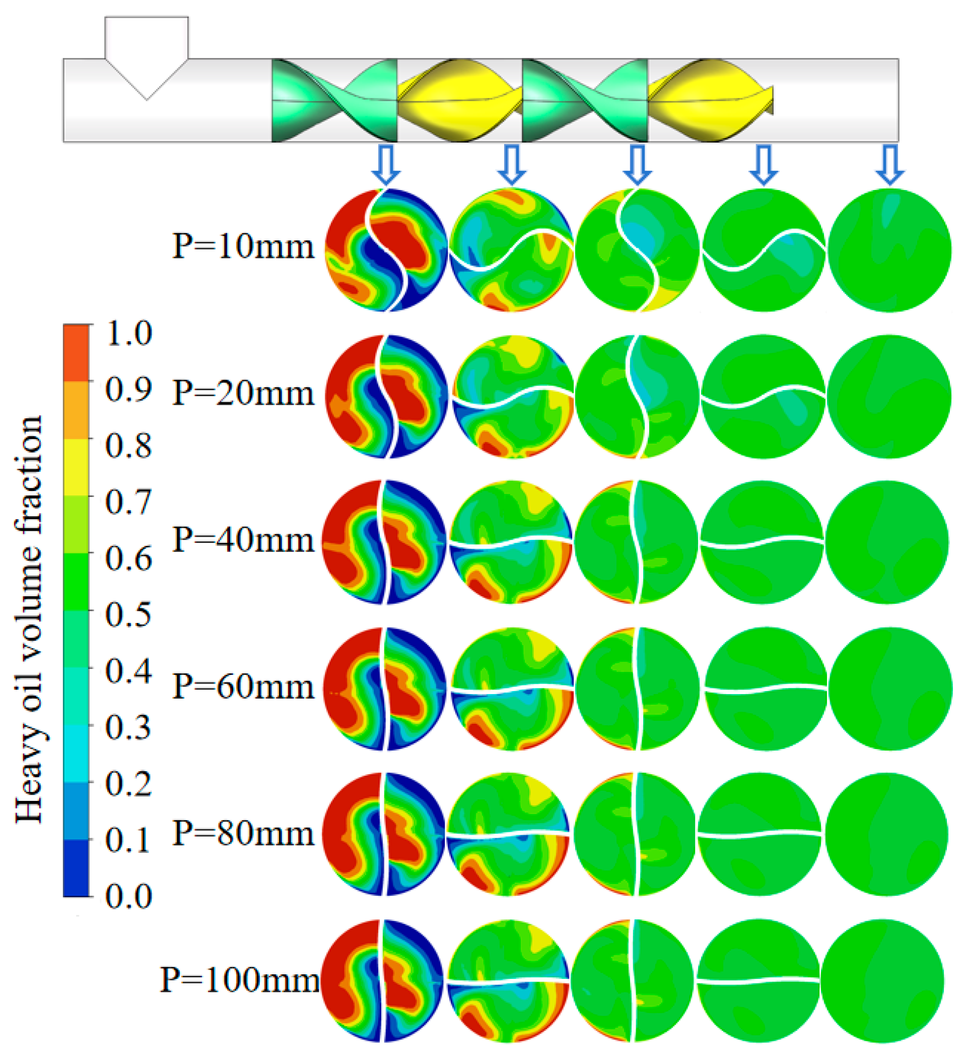
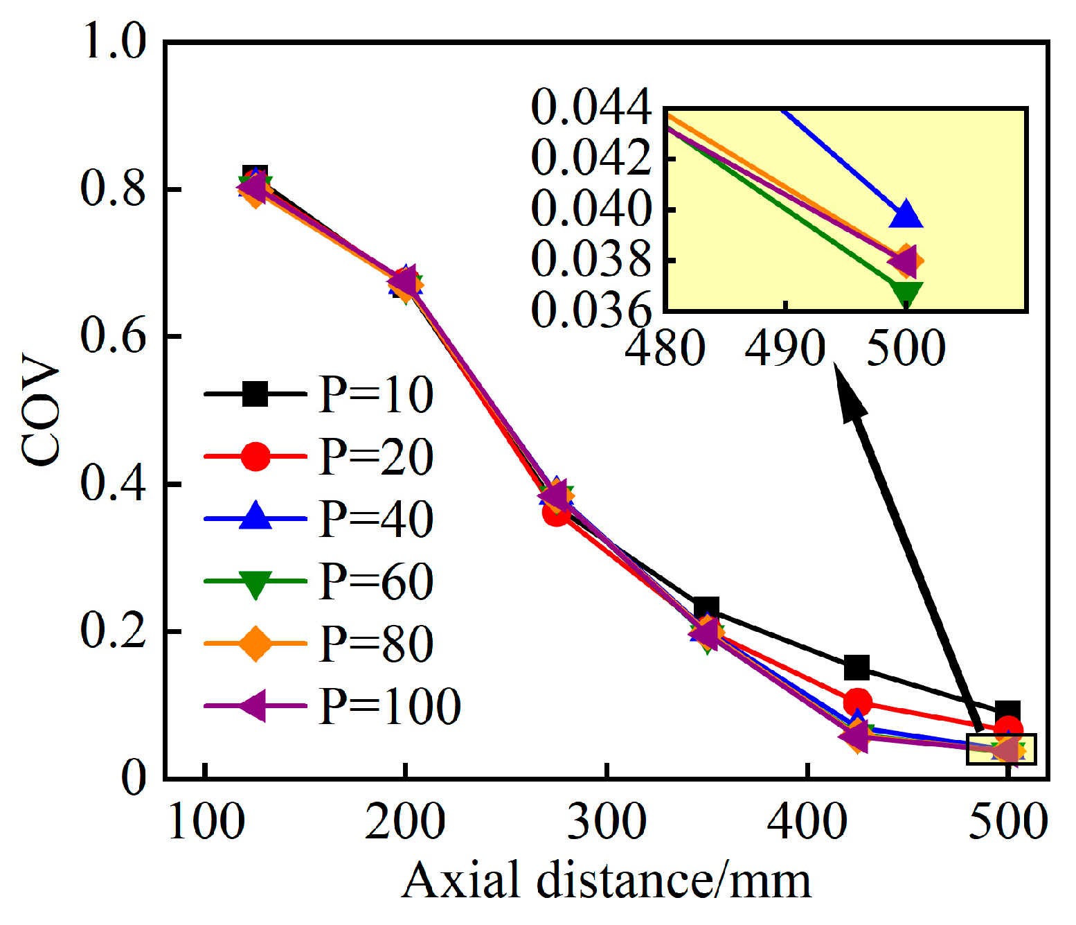
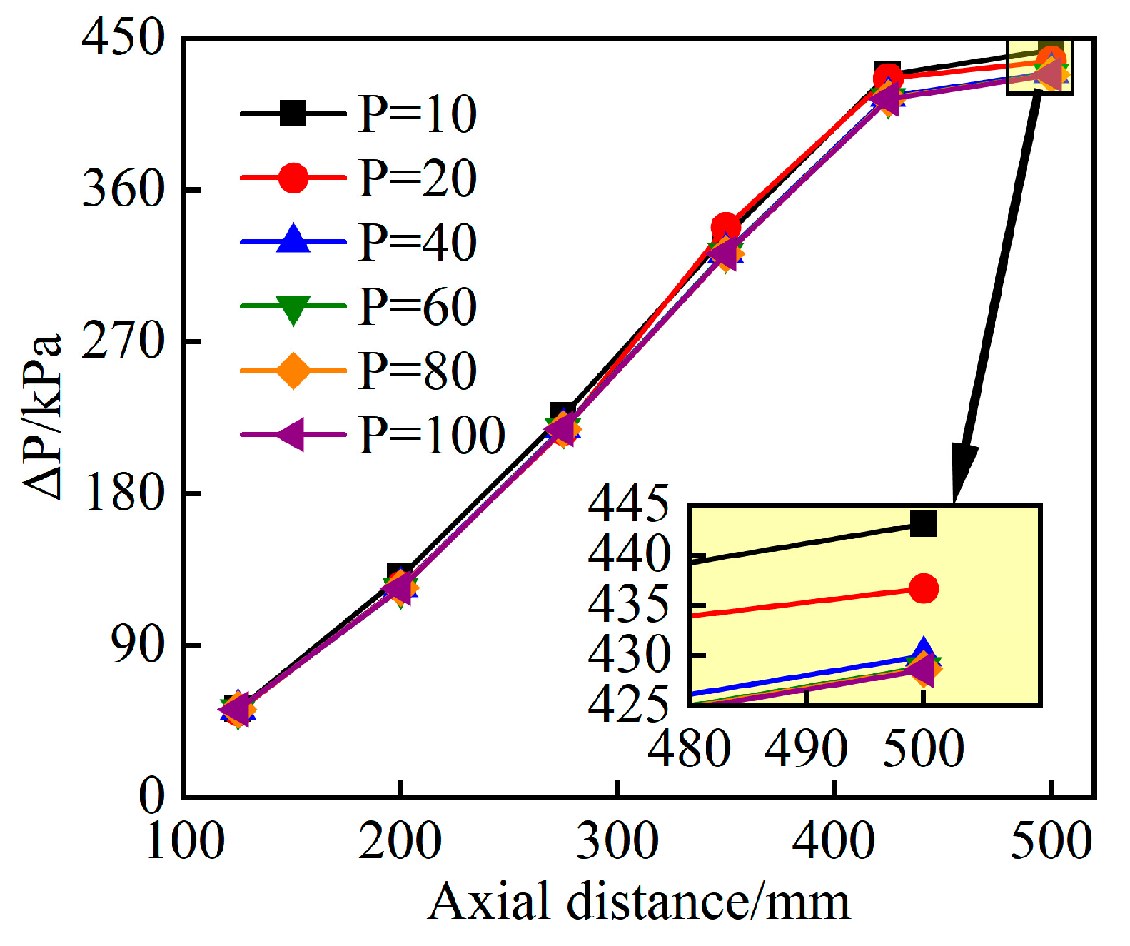
3.2. Influence of Focal Length P on Mixing Performance

According to Equation (1), the slope of the parabola is influenced by the focal length P, which subsequently affects the surface area of the parabolic blade. To investigate the influence of P on the mixing performance of the parabolic static mixer, simulations were conducted for parabolic static mixers with varying P values of 10 mm, 20 mm, 40 mm, 60 mm, 80 mm, and 100 mm, under structural parameters of α = 180° and Ar = 1.5. Cross sections at axial distances of 200 mm, 275 mm, 350 mm, 425 mm, and 500 mm were analyzed to evaluate the volume fraction of heavy oil, as shown in Figure 11. When P is 10 mm and 20 mm, the mixing effect is suboptimal. At the outlet of the fourth parabolic blade, a high-concentration zone of light oil persists, and for P = 10 mm, this high-concentration zone extends to the pipeline outlet. When P > 20 mm, the mixture of heavy oil and light oil becomes relatively uniform at the outlet of the fourth parabolic blade, resulting in the absence of a high-concentration zone.

Figure 12 illustrates the variation of the COV with axial distance for parabolic static mixers at different P values. The COV for parabolic static mixers exhibited an overall downward trend. In the first three mixing blades, the influence of different P values on the COV was minimal, with the COV reaching approximately 0.2. After the mixed fluid passed through the three mixing blades, the COV values began to exhibit significant differences. The rate of decrease in the COV for P ≤ 20 mm was slower than that for P > 20 mm, resulting in a suboptimal mixing effect at the pipe outlet. However, when P > 20 mm, the COV values fell below 0.05, indicating that heavy oil and light oil achieved nearly complete mixing. Nevertheless, excessive P reduces the strength of the fluid swirl, resulting in the parabolic static mixer with P = 60 mm, demonstrating the optimal mixing effect at the pipe outlet.

Figure 13 illustrates the variation of ∆P in a parabolic static mixer with axial distance at different P values. The effect of P on the pressure drop of the parabolic static mixer is relatively minor. As the axial distance increases, ∆P gradually rises and tends to stabilize after the fourth mixing blade. As the P value increases, the blade opening increases and its curvature decreases, leading to a reduction in the contact area between the mixed fluid and the blade. This, in turn, decreases the resistance in the fluid path, resulting in a corresponding reduction in ∆P. The parabolic static mixer with P = 10 mm exhibited the largest ∆P, reaching 443.2 kPa. Conversely, the parabolic static mixer at P = 100 mm produced the smallest ∆P, measuring 428.6 kPa.

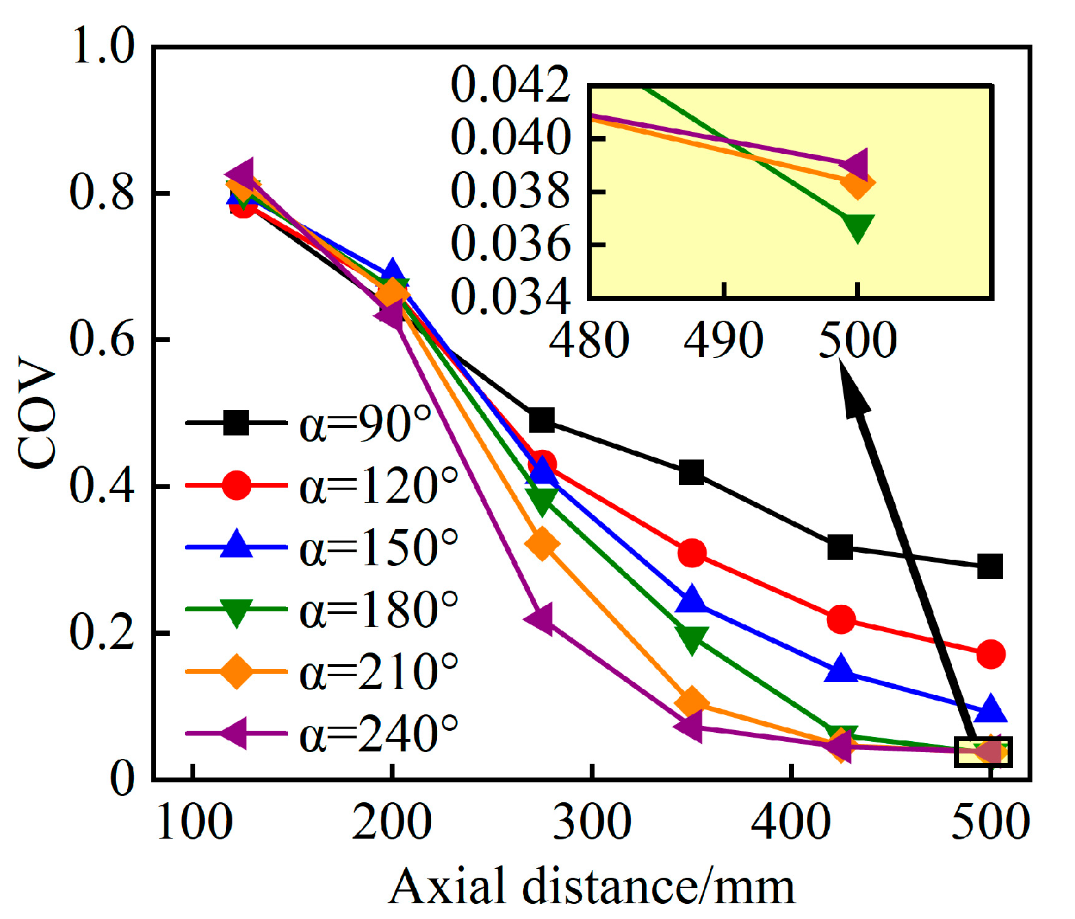
3.3. Influence of Torsion Angle α on Mixing Performance

To investigate the influence of α on the mixing performance of parabolic static mixers, numerical simulations were conducted for parabolic static mixers with α values of 90°, 120°, 150°, 180°, 210°, and 240°, while maintaining structural parameters of P = 60 mm and Ar = 1.5. Figure 14 presents the mixing effects observed in the axial cross sections of the mixer at different α values. When α < 150°, the mixing effect of the parabolic static mixer is suboptimal, with a noticeable high-concentration zone of heavy oil remaining at the pipeline outlet. At α = 150°, although a slight uneven mixing phenomenon is observed at the outlet of the fourth mixing blade, the enhanced swirl effect improves the overall mixing performance, resulting in the absence of a high-concentration area at the outlet. When α > 150°, the mixing effect of heavy oil and light oil significantly improves after passing through the fourth mixing blade, with no high-concentration zone observed.

Figure 15 illustrates the variation of the COV with axial distance for parabolic static mixers at different α values. At the outlet of the first mixing blade, the COV values for the parabolic static mixers with varying α values exhibit minimal differences, remaining approximately at 0.7. As the mixing process advances, the COV decreases with increasing α in the second mixing blade region. The larger α is, the faster the COV decreases, indicating that increasing the torsion angle can significantly enhance the mixing efficiency of heavy oil and light oil. In the region between the third and fourth mixing blades, the rate of decrease in the COV for each mixer slows down, and as α increases, the COV stabilizes more rapidly. At the pipeline outlet, when α ≤ 150°, larger α values correspond to smaller COV values. When α > 150°, the COV falls below 0.05, indicating that heavy oil and light oil are nearly completely mixed. However, with larger α values, energy consumption in the mixing region increases, hindering swirl development and reducing the axial velocity. As a result, the COV cannot be reduced further after passing through the fourth mixing blade. Consequently, smaller α values correspond to lower COV values, with the parabolic static mixer at α = 180° achieving the best mixing effect.

Figure 16 illustrates the variation of ∆P in a parabolic static mixer with axial distance at different α values. ∆P increases as α increases, with larger α values resulting in a faster rise in ∆P. An increase in α results in a larger contact area between the fluid and the blade, thereby increasing resistance in the fluid path. Additionally, at the same axial distance, a higher α compels the mixed fluid to undergo a greater angular twist, which requires more energy and contributes to a further increase in ∆P. The parabolic static mixer with α = 240° exhibits the largest ∆P, reaching 581.1 kPa, while the smallest ∆P occurs at α = 90°, measuring 287.3 kPa.

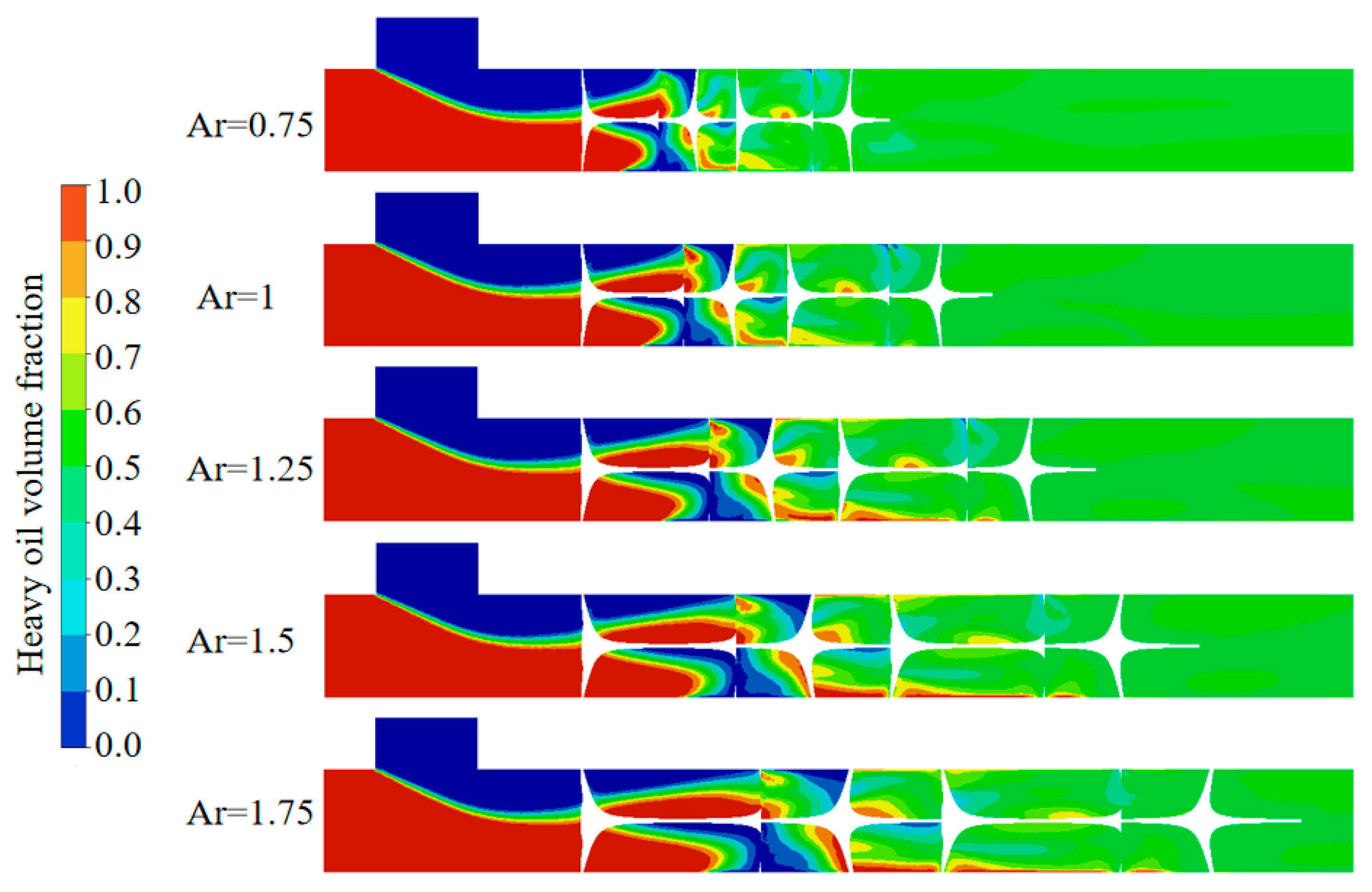
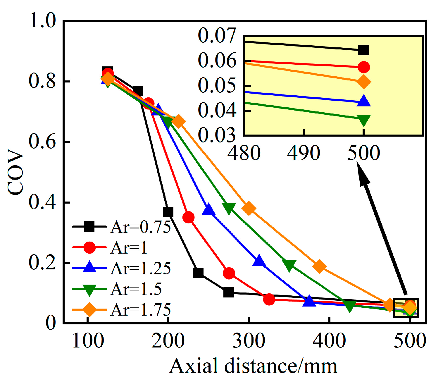
3.4. Influence of Length-to-Diameter Ratio Ar on Mixing Performance

Since the inner diameter of the mixing pipe is fixed, changes in Ar indirectly alter the axial length of the mixing blade, subsequently affecting the length of the mixing region. To investigate the effect of Ar on the mixing performance of parabolic static mixers, numerical simulations were conducted for parabolic static mixers with Ar values of 0.75, 1, 1.25, 1.5, and 1.75, under the structural parameters P = 60 mm and α = 180°. Axial sections were analyzed to compare the mixing effects of static mixers at different Ar values, as illustrated in Figure 17. Ar has minimal influence on the mixing performance of the parabolic static mixer. When Ar ≤ 1, no high-concentration zone of heavy oil is observed in the fourth mixing blade region. When Ar > 1, although a high-concentration zone of heavy oil is present in the fourth mixing blade region, further mixing leads to uniform mixing of heavy oil and light oil at the outlet of the mixing blade.

The effect of Ar on the dilution mixing process of heavy oil was further analyzed by examining the change in the COV with axial distance, as illustrated in Figure 18. Inside the mixing region, parabolic static mixers with varying Ar values exhibited significant differences in mixing rates. As Ar decreases, the COV exhibits a downward trend; smaller Ar values correspond to a faster decline rate of the COV and a shorter axial distance required to achieve a stable state. At the outlet of the fourth mixing blade, although the COV increases with decreasing Ar, the differences in the COV among the various Ar values are not significant. This indicates that while different Ar values have a greater impact on the mixing process of the parabolic static mixer, their effect on the final mixing outcome is relatively minor. Following the fourth mixing blade, the COV of parabolic static mixers with different Ar values gradually stabilized; however, it continued to exhibit a downward trend due to the ongoing mixing of heavy oil and light oil. Notably, when Ar > 1.25, the COV of the parabolic static mixer decreases more rapidly, indicating that larger Ar values enhance the swirl strength of the mixed fluid generated by the mixing blade. Even after the influence of the mixing blade diminishes, the COV continues to decline at a certain rate. The parabolic static mixer with Ar = 1.5 demonstrates the optimal mixing performance.

Figure 19 illustrates the variation of ∆P in parabolic static mixers with axial distance under different Ar conditions. ∆P in parabolic static mixers increases as Ar decreases, and within the blade mixing region, smaller Ar values result in a more rapid increase in ∆P. When the mixed fluid passes through the first mixing blade, it experiences shear action that induce a swirling motion. In the case of small Ar values, the mixed fluid must achieve 180° of torsion over a short distance, which significantly increases axial resistance. Additionally, since the swirl is not fully developed, it is shunted and merged by the second mixing blade, resulting in increased shear resistance at the blade junction. Consequently, energy consumption increases significantly, even when rapid mixing occurs over shorter distances. This also explains why the COV of the parabolic static mixer drops slowly in the outlet of the blade mixing region when Ar ≤ 1.25. The parabolic static mixer with Ar = 0.75 exhibited the highest ∆P, reaching 769.4 kPa. Conversely, the parabolic static mixer with Ar = 1.75 yielded the lowest ∆P, measuring 404.4 kPa.

4. Conclusions

This study proposes an innovative parabolic blade design to replace the traditional Kenics blade. The two static mixers were compared and analyzed using Fluent software, focusing on three key parameters of the parabolic blade. The purpose of this study is to investigate the influence of the parabolic static mixer on the performance of the heavy oil dilution mixing process. The conclusions are summarized as follows:

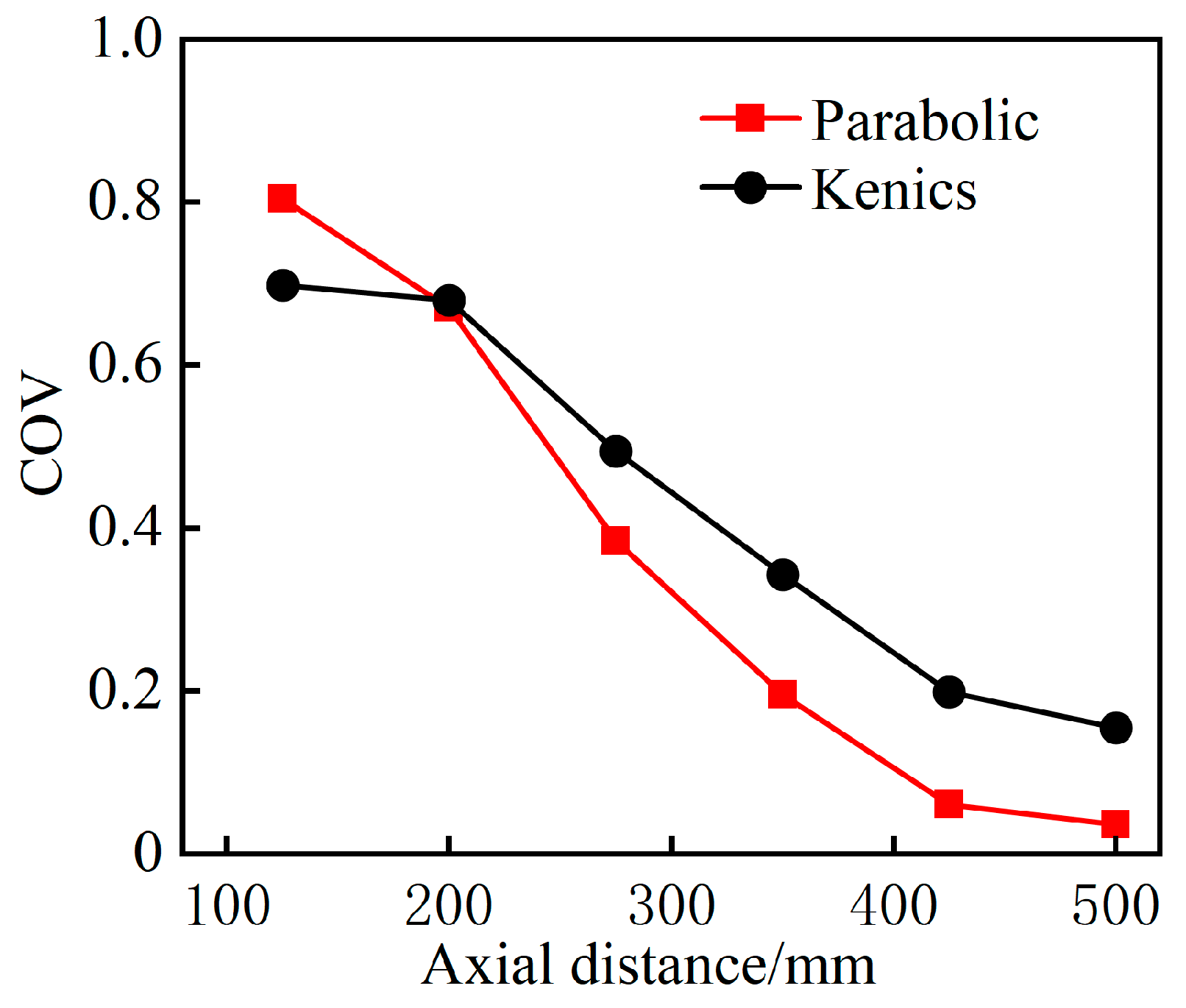
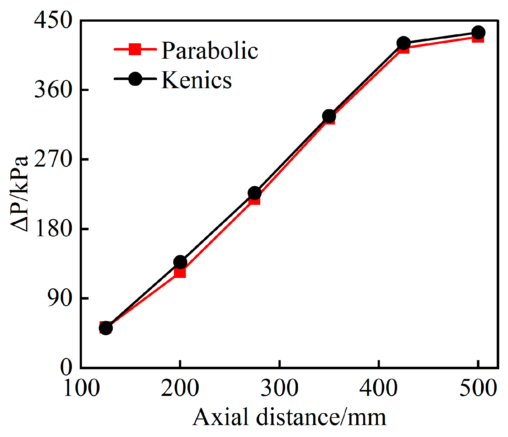
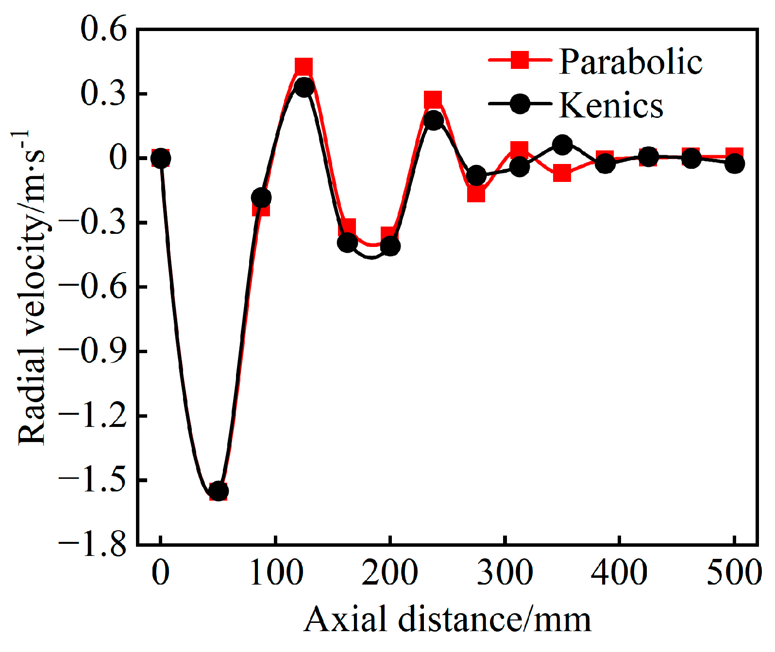
• Comparative analysis reveals that the mixing performance of the parabolic static mixer is significantly different from that of the traditional Kenics static mixer. The parabolic blade considerably improves radial velocity fluctuations and enhances turbulent kinetic energy, thereby promoting both radial and axial mixing of heavy oil and light oil. Consequently, the coefficient of concentration variance (COV) of the parabolic static mixer can be reduced to 0.036. This results in nearly complete mixing of heavy oil and light oil, while the pressure drop (∆P) is also slightly reduced.
• As P increases, the path resistance correspondingly decreases, leading to a reduction in the pressure drop (∆P) and thereby enhancing the mixing effect of the parabolic static mixer. However, when P is excessively high, the curvature of the parabola decreases, which weakens the swirling effect of the mixed fluid. The parameter P has little influence on the ΔP of the parabolic static mixer, so the COV is used as the main evaluation index. Considering all factors, the parabolic static mixer with P = 60 mm exhibits the best mixing performance.
• As α increases, the swirl intensity rises, leading to a decrease in the COV of the parabolic static mixer. However, when α becomes excessively large, the torsion angle of the mixed fluid increases over the same distance, resulting in a rise in ∆P and a decrease in axial velocity, thereby weakening the mixing performance at the outlet of the mixer. In order to ensure good mixing effect and a minimum pressure drop, comprehensive analysis shows that the parabolic static mixer with α = 180° has the best mixing performance.
• Different Ar values significantly influence the mixing process of parabolic static mixers. The smaller Ar is, the faster the COV decreases, resulting in a shorter axial distance to reach a stable state. However, excessively small Ar values can cause a sharp increase in ∆P over a short distance due to blade swirl and shear action, significantly increasing energy consumption and adversely affecting the mixing performance. Considering all factors, the parabolic static mixer with Ar = 1.5 exhibits the best mixing performance.

References

1. Gateau, P.; Hénaut, I.; Barré, L.; Argillier, J.F. Heavy oil dilution. Oil Gas Sci. Technol. 2004, 59, 503–509. [Google Scholar] [CrossRef]
2. Gao, X.D.; Dong, P.C.; Cui, J.W.; Gao, Q.C. Prediction Model for the Viscosity of Heavy Oil Diluted with Light Oil Using Machine Learning Techniques. Energies 2022, 15, 2297. [Google Scholar] [CrossRef]
3. Wang, Q.X.; Zhang, W.; Wang, C.; Han, X.D.; Wang, H.Y.; Zhang, H. Microstructure of Heavy Oil Components and Mechanism of Influence on Viscosity of Heavy Oil. ACS Omega 2023, 8, 10980–10990. [Google Scholar] [CrossRef]
4. Hasan, S.W.; Ghannam, M.T.; Esmail, N. Heavy crude oil viscosity reduction and rheology for pipeline transportation. Fuel 2010, 89, 1095–1100. [Google Scholar] [CrossRef]
5. Martinez-Palou, R.; Mosqueira, M.d.L.; Zapata-Rendon, B.; Mar-Juarez, E.; Bernal-Huicochea, C.; Clavel-Lopez, J.d.l.C.; Aburto, J. Transportation of heavy and extra-heavy crude oil by pipeline: A review. J. Pet. Sci. Eng. 2011, 75, 274–282. [Google Scholar] [CrossRef]
6. Thakur, R.K.; Vial, C.; Nigam, K.D.P.; Nauman, E.B.; Djelveh, G. Static mixers in the process industries—A review. Chem. Eng. Res. Des. 2003, 81, 787–826. [Google Scholar] [CrossRef]
7. Liu, C.-W.; Wei, H.-B.; Li, Z.-M. Numerical Simulation of the Influence of Swirl Mixer on Effect of Blending Dilute Oil through Oil Tube. Sci. Technol. Eng. 2012, 12, 3848–3851. [Google Scholar] [CrossRef]
8. Fei, X. Simulation Study on Flow in Xinjiang Heavy Oil Mixed with Dilute Riser. Master Thesis, Southwest Petroleum University, Chengdu, China, 2014. [Google Scholar]
9. Wang, X.; Zhao, C.; Han, W.; Zhou, Y. Numerical Simulation of the Down Hole Static Mixer for Heavy Oil Thin Mixing. J. Chongqing Univ. Sci. Technol. 2015, 17, 50–53+84. [Google Scholar] [CrossRef]
10. Li, Q.; Peng, Y.; Huang, Z.; Qiu, C.; Jin, Y.; Wang, N. Numerical Simulation of the Downhole Dynamic Mixer for Heavy Oil Thin Mixing. China Pet. Mach. 2014, 42, 72–76. [Google Scholar] [CrossRef]
11. Shi, C.W.; Yang, W.; Chen, J.B.; Sun, X.P.; Chen, W.Y.; An, H.Y.; Duo, Y.L.; Pei, M.Y. Application and mechanism of ultrasonic static mixer in heavy oil viscosity reduction. Ultrason. Sonochem. 2017, 37, 648–653. [Google Scholar] [CrossRef]
12. Zhang, Y.; Peng, Z.-H.; Gao, D.-X.; Ren, H.-T.; Tang, Y.-X. Design and mixing performance research of core tube heavy oil mixing and diluting mixer. Chin. J. Eng. Des. 2018, 25, 510–517. [Google Scholar] [CrossRef]
13. Zheng, L.; Lan, D.; Yang, Z.Y. Research on numerical simulation of the casing pipe blending lightoil for heavy oil dilution wells. Chin. J. Hydrodyn. 2018, 33, 609–617. [Google Scholar] [CrossRef]
14. Wan, J.; Lin, R.; Ge, Y.; Dai, B.; Chen, X.; Huang, S.; Wang, L.; Liu, E. Numerical simulation of the effect of kenics type static mixer on the homogenization effect of water-cut crude oil. Chem. Eng. Oil Gas. 2024, 53, 83–89. [Google Scholar]
15. Rahimi, M. The effect of impellers layout on mixing time in a large-scale crude oil storage tank. J. Pet. Sci. Eng. 2005, 46, 161–170. [Google Scholar] [CrossRef]
16. Wang, Z.; Wang, L.; Meng, H. CFD-PBM numerical simulation on the breakup and coalescence process of dispersed phase droplet in Kenics static mixer. Chin. J. Process Eng. 2021, 21, 935–943. [Google Scholar] [CrossRef]
17. Zhang, C.; Yang, P.; Liu, L. Influence of the Arrangement Angle of the Blade on the Mixing Effect of the Three-Spiral Static Mixer. Plastics 2023, 52, 87–91. [Google Scholar]
18. Tang, Y.; Xie, L.; Zhu, S.; Xu, J.; Xiang, S. Effect of perforation on mixing performance of perforated Kenics static mixer. Petrochem. Technol. 2024, 53, 670–677. [Google Scholar] [CrossRef]
19. Meng, L.C.; Gao, X.F.; Wang, D.W.; Liu, Y.; Wang, R.J.; Hu, B.S.; Tang, M.; Zhang, S.F. Experimental study on energy consumption characteristics of rotational-perforated static mixers. Can. J. Chem. Eng. J. Chem. Eng. 2023, 101, 6656–6671. [Google Scholar] [CrossRef]
20. Deng, M.; Zhou, C.; Zhang, Y.; Ren, H.; Li, H. Research of the Heavy Oil Mixer with Helical-jet Mode. In Proceedings of the 2019 6th International Conference on Machinery, Mechanics, Materials, and Computer Engineering (MMMCE 2019), Hohhot, China, 27–28 July 2019; p. 9. [Google Scholar]
21. Chen, H.Y.; Zhang, J.; Ji, Y.; Zhou, J.W.; Hu, W.B. Numerical Simulation of Internal Flow Field in Optimization Model of Gas-Liquid Mixing Device. Processes 2024, 12, 1707. [Google Scholar] [CrossRef]
22. Wang, Y.; Han, H.; Liang, Z.; Yang, H.; Li, F.; Zhang, W.; Zhao, Y. Analysis of the Effect of Structural Parameters on the Internal Flow Field of Composite Curved Inlet Body Hydrocyclone. Processes 2024, 12, 2654. [Google Scholar] [CrossRef]
23. Liu, Y.H.; Gao, M.M.; Huang, Z.B.; Wang, H.F.; Yuan, P.Q.; Xu, X.R.; Yang, J.Y. Numerical Simulation of the Mixing and Salt Washing Effects of a Static Mixer in an Electric Desalination Process. Processes 2024, 12, 883. [Google Scholar] [CrossRef]
24. Chen, G.H.; Liu, Z.L. Numerical Research of Pressure Drop in Kenics Static Mixer. In Proceedings of the 4th International Conference on Manufacturing Science and Engineering (ICMSE 2013), Dalian, China, 30–31 March 2013; pp. 547–550. [Google Scholar]
25. Brazhenko, V.; Qiu, Y.B.; Mochalin, I.; Zhu, G.G.; Cai, J.C.; Wang, D.Y. Study of hydraulic oil filtration process from solid admixtures using rotating perforated cylinder. J. Taiwan Inst. Chem. Eng. 2022, 141, 104578. [Google Scholar] [CrossRef]
Figure 1. Geometric model of mixing blades: (a) Parabolic blade; (b) Traditional Kenics blades.
Processes 13 01125 g001
Figure 2. Parabolic static mixer model.
Processes 13 01125 g002
Figure 3. Mesh division of parabolic static mixer.
Processes 13 01125 g003
Figure 4. Mesh independence verification.
Processes 13 01125 g004
Figure 5. Z factor verification by empirical model.
Processes 13 01125 g005
Figure 6. Distribution of heavy oil volume fraction in the axial section of the static mixer: (a) Parabolic static mixer; (b) Traditional Kenics static mixer.
Processes 13 01125 g006
Figure 7. The COV varies with axial distance.
Processes 13 01125 g007
Figure 8. ∆P varies with axial distance.
Processes 13 01125 g008
Figure 9. The radial velocity varies with axial distance.
Processes 13 01125 g009
Figure 10. The turbulent kinetic energy varies with axial distance.
Processes 13 01125 g010
Figure 11. Distribution of heavy oil volume fraction in static mixer cross section.
Processes 13 01125 g011
Figure 12. The COV varies with the axial distance.
Processes 13 01125 g012
Figure 13. ∆P varies with the axial distance.
Processes 13 01125 g013
Figure 14. Distribution of heavy oil volume fraction in cross-section of static mixer.
Processes 13 01125 g014
Figure 15. The COV varies with axial distance.
Processes 13 01125 g015
Figure 16. ∆P varies with axial distance.
Processes 13 01125 g016
Figure 17. Distribution of heavy oil volume fraction in axial section.
Processes 13 01125 g017
Figure 18. COV varies with the axial distance.
Processes 13 01125 g018
Figure 19. ∆P varies with the axial distance.
Processes 13 01125 g019