
Research on the Development Potential of a Hybrid Energy Electric–Hydrogen Synergy System: A Case Study of Inner Mongolia

Abstract
:1. Introduction
- Objective Perspective: For example, reference [5] employs the Anti-Entropy Weights (AEWs) method to determine indicator weights, while reference [6] utilizes the CRITIC method to evaluate photovoltaic energy system indicators. While deriving their weights from inherent data patterns, these approaches do not systematically account for decision-makers’ preferences in the weighting calculus.
- Subjective Perspective: Reference [7] combines the Grey Decision-Making Trial and Evaluation Laboratory (Grey-DEMATEL) method with the Fuzzy Analytic Hierarchy Process (Fuzzy-AHP) to determine indicator weights. Similarly, reference [8] uses cloud models and fuzzy techniques to rank the importance of the indicators. Although anchored in expert judgments, such subjective methods’ absence of data-driven validation could compromise decision robustness due to cognitive bias propagation.
- Huber-adapted gradients dynamically modulate the update magnitudes;
- Iterative refinement converges to consensus weights through error-adaptive learning.
2. Materials and Methods
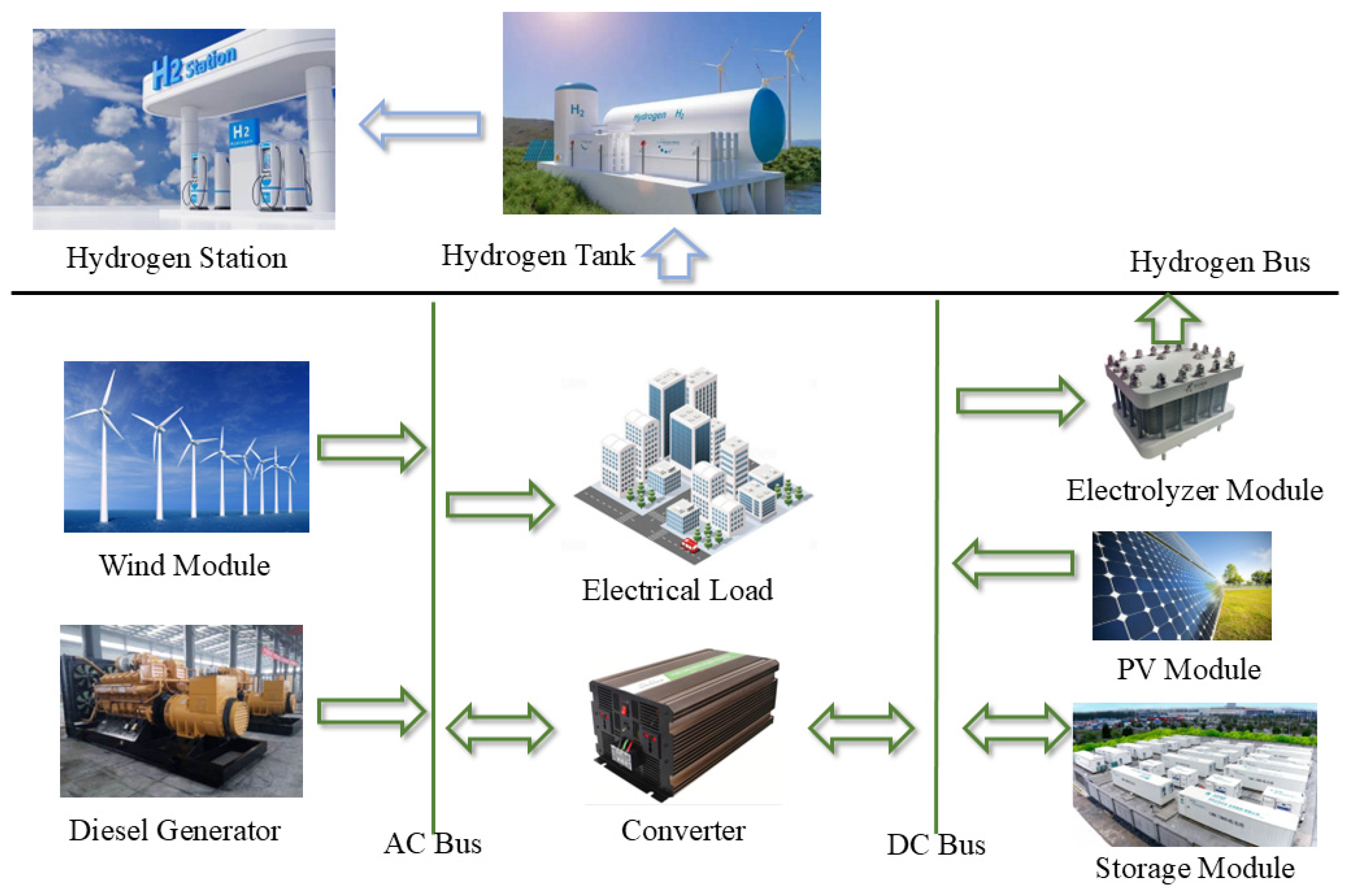
2.1. Construction of Hybrid Energy Electric–Hydrogen Collaborative System
2.2. Index Evaluation System
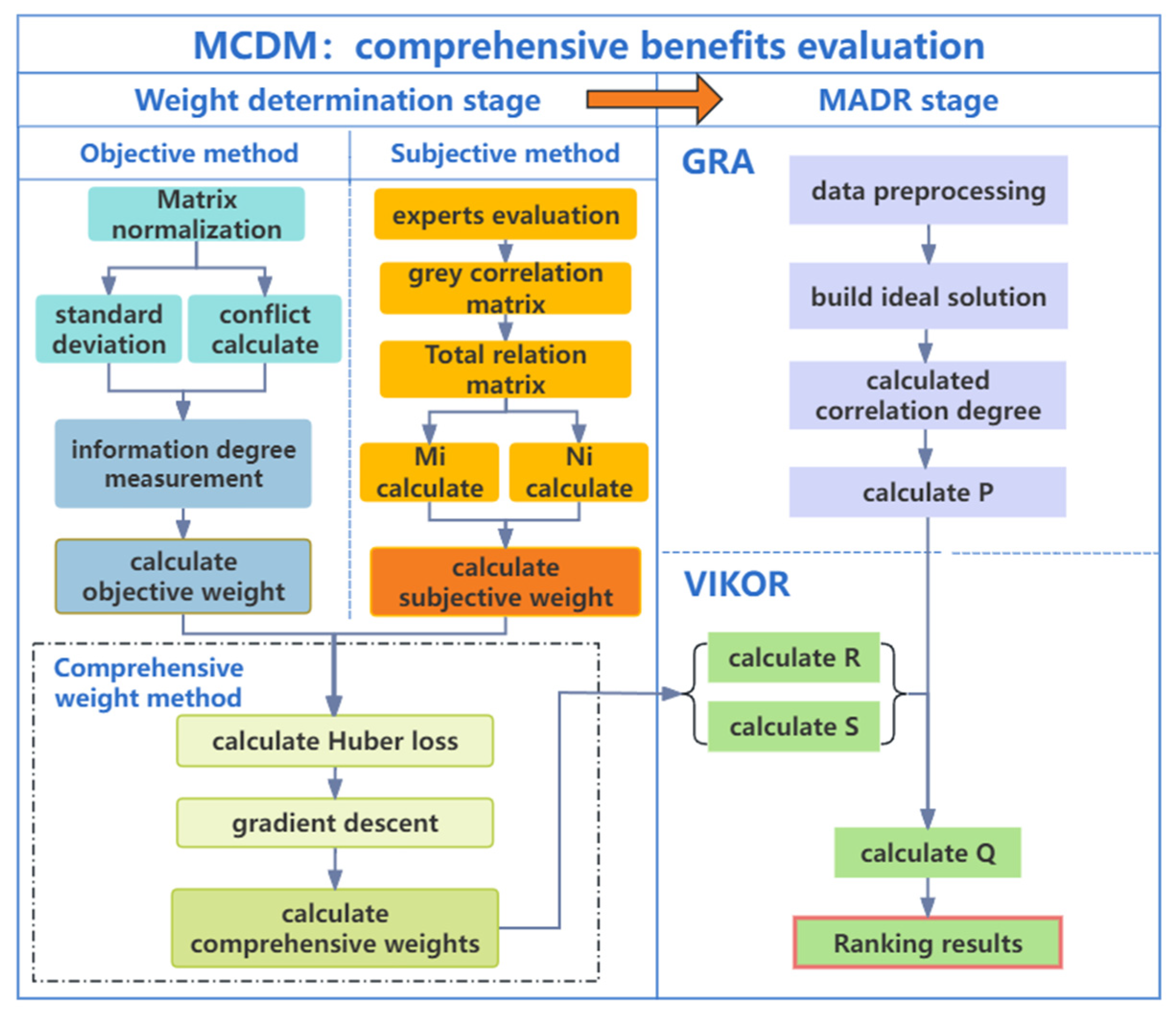
2.3. Comprehensive Benefit Evaluation Model
2.3.1. Subjective Evaluation Based on CRITIC Method
2.3.2. Objective Evaluation Based on GREY-DEMATEL Method
2.3.3. Comprehensive Evaluation Based on Conflict Scenarios
2.3.4. Scheme Ranking Method Based on GRA-VIKOR
3. Example Calculation and Result Analysis
3.1. Example Information
3.2. Homer Simulation Result
3.3. Indicators’ Weight Results
3.4. GRA-VIKOR Ranking Results
4. Discussion
4.1. Validation of Model
4.2. Case Disparity Analysis
4.3. Analysis of Simulation Results
5. Conclusions
Author Contributions
Funding
Data Availability Statement
Conflicts of Interest
Appendix A
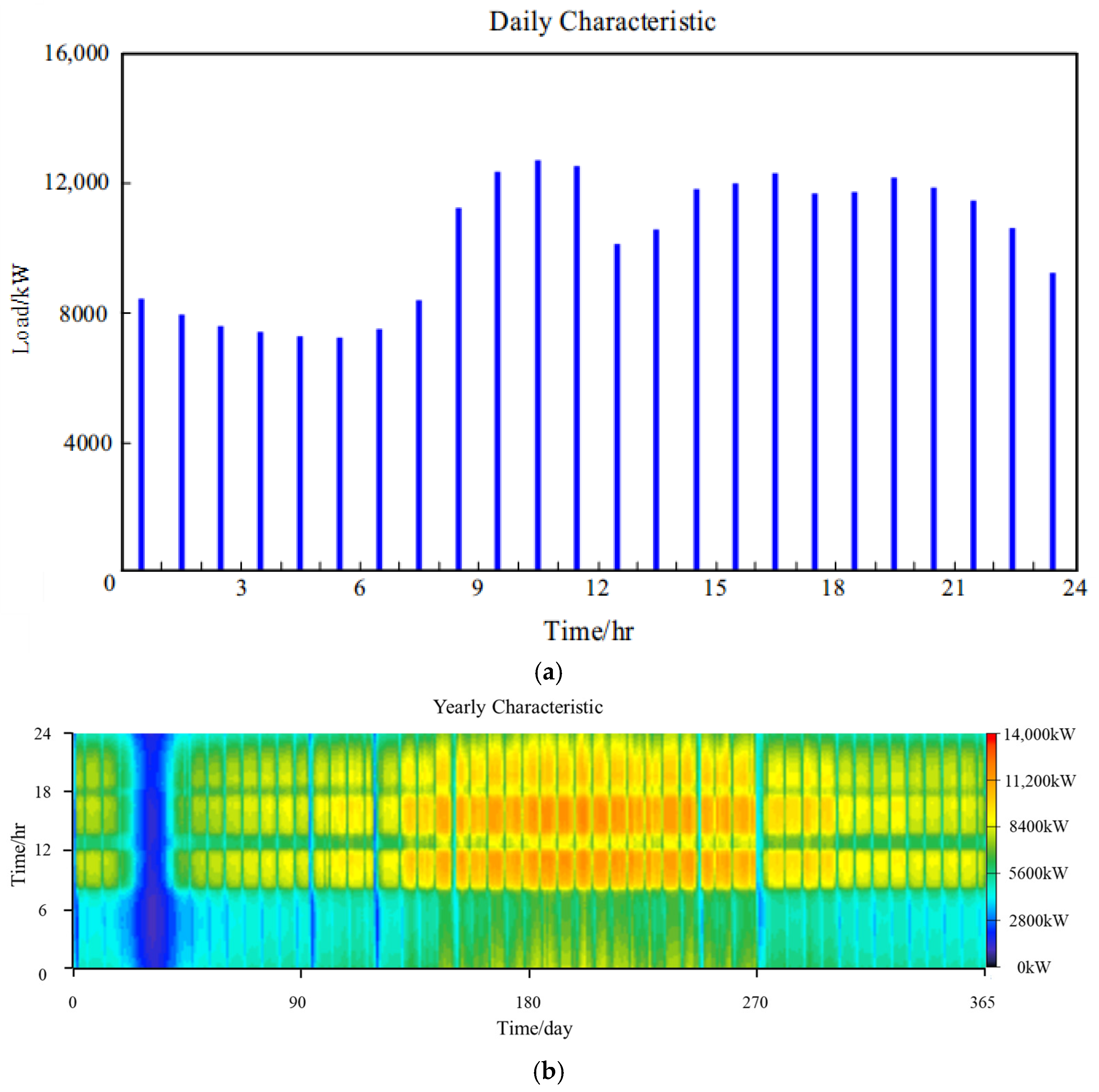
Appendix A.1. Load Scenarios
- (1)
- Electrical Load:
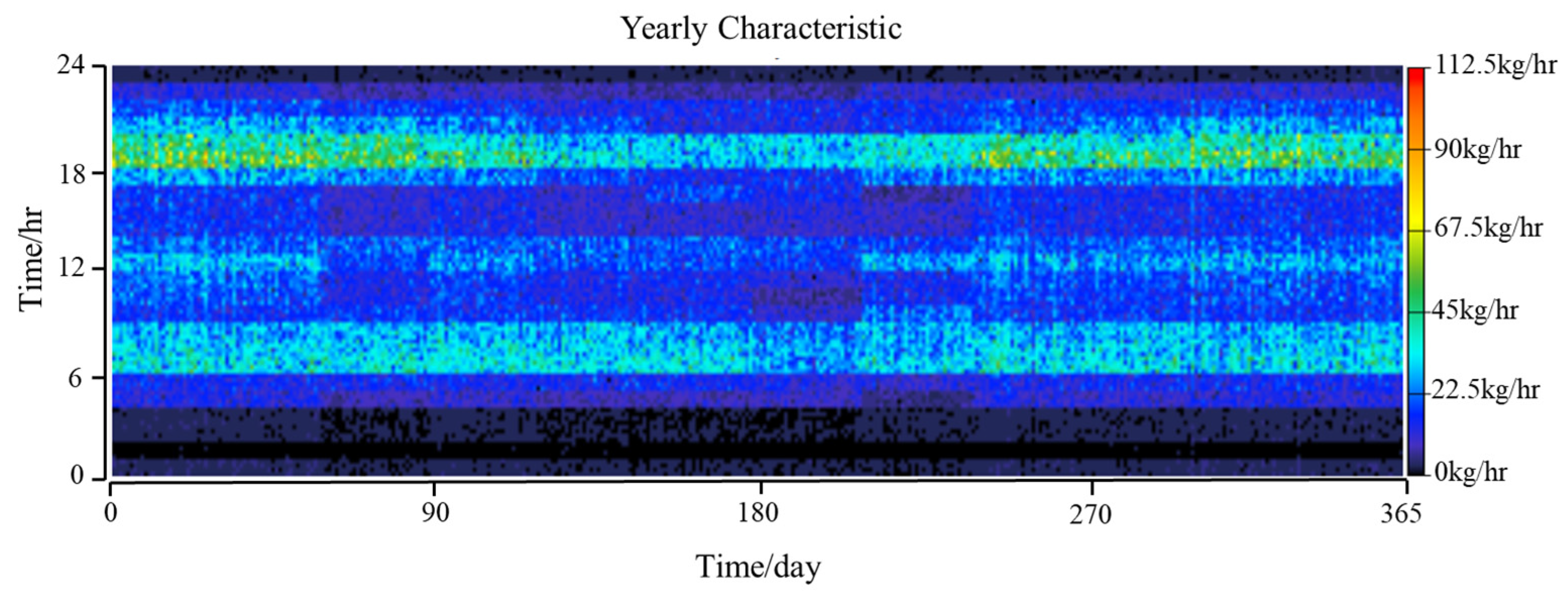
- (2)
- Hydrogen Load:

Appendix A.2. Modelling of System Components
- (1)
- Wind Turbines:
- (2)
- Solar Photovoltaic (PV) Panels:
- (3)
- Diesel Generator:

| Carbon Dioxide (g/L Fuel) | Carbon Monoxide (g/L Fuel) | Unburned Hydrocarbons (g/L Fuel) | PMx (g/L Fuel) | NOx (g/L Fuel) | Sulphur Dioxide (g/L Fuel) |
|---|---|---|---|---|---|
| 2617.5 | 16.5 | 0.72 | 0.1 | 15.5 | 15.5 |
- (4)
- Electrolyzer:
- (5)
- Rectifier–Inverter Unit:
- (6)
- Energy Storage System:
| Component | Capital Cost (CNY/kW) | Replacement Cost (CNY/kW) | O&M COST (CNY/yr) | Lifetime (yr) | Connection |
|---|---|---|---|---|---|
| Wind Turbine | 6200 | 6000 | 1830 | 20 | AC |
| Diesel Generator | 4000 | 3740 | 0.03 | 11 | DC |
| PV | 5230 | 4950 | 30 | 25 | DC |
| Electrolyzer | 10,867 | 9500 | 215 | 25 | DC |
| Converter | 920 | 825.8 | 7.24 | 15 | / |
| Storage Module | 150 | 102 | 2 | 15 | DC |
| Hydrogen Tank | 3750.5 | 3500 | 3.93 | 15 | DC |
References
- Hassan, Q.; Sameen, A.Z.; Olapade, O.; Alghoul, M.; Salman, H.M.; Jaszczur, M. Hydrogen fuel as an important element of the energy storage needs for future smart cities. Int. J. Hydrogen Energy 2023, 48, 30247–30262. [Google Scholar] [CrossRef]
- Zhang, M.; Cong, N.; Song, Y.; Xia, Q. Cost analysis of onshore wind power in China based on learning curve. Energy 2024, 291, 130459. [Google Scholar] [CrossRef]
- Cui, J.; Aziz, M. Optimal design and system-level analysis of hydrogen-based renewable energy infrastructures. Int. J. Hydrogen Energy 2024, 58, 459–469. [Google Scholar] [CrossRef]
- Zhang, G.; Ren, J.; Zeng, Y.; Liu, F.; Wang, S.; Jia, H. Security assessment method for inertia and frequency stability of high proportional renewable energy system. Int. J. Electr. Power Energy Syst. 2023, 153, 109309. [Google Scholar] [CrossRef]
- Wen, M.; Liu, Y.; Hu, X.; Cheng, H. Evaluation of Integrated Energy System Planning with Distributed Functional Devices. Electr. Meas. Instrum. 2018, 55, 68–74. [Google Scholar]
- Ilham, N.; Dahlan, N.Y.; Hussin, M.Z. Optimizing solar PV investments: A comprehensive decision-making index using CRITIC and TOPSIS. Renew. Energy Focus 2024, 49, 100551. [Google Scholar] [CrossRef]
- Gupta, S.; Kumar, R.; Kumar, A. Green hydrogen in India: Prioritization of its potential and viable renewable source. Int. J. Hydrogen Energy 2024, 50, 226–238. [Google Scholar] [CrossRef]
- Xu, C.; Yang, J.; LI, X. Research on the Construction of Comprehensive Evaluation Index System for Renewable Energy Hydrogen Production Projects Aimed at Carbon Neutrality. Proj. Manag. Technol. 2022, 20, 108–112. [Google Scholar]
- Altintas, E.; Utlu, Z. Planning energy usage in electricity production sector considering environmental impacts with fuzzy TOPSIS method & game theory. Clean. Eng. Technol. 2021, 5, 100283. [Google Scholar]
- Qian, J.; Wu, J.; Yao, L.; Mahmut, S.; Qiang, Z. Comprehensive Performance Evaluation of CCHP-PV-Wind System Based on Exergy Analysis and Multi-objective Decision-making Method. Power Syst. Prot. Control 2021, 49, 130–139. [Google Scholar]
- Feng, X.; Zhang, S.; Zhu, T.; Shao, H.; Liu, Y.; Miao, S. Analysis of Large-scale Energy Storage Selection Based on Interval Type-2 Fuzzy Multi-attribute Decision-making Method. High Volt. Eng. 2021, 47, 4123–4136. [Google Scholar]
- Ma, Z.; Zhao, H.; Huo, H.; Lu, H. Comprehensive Evaluation of User Energy Storage System Configuration Scheme Based on Improved Triangular Fuzzy VIKOR Method. Electr. Power 2022, 55, 185–191. [Google Scholar]
- Ansari, A.B. Multi-objective size optimization and economic analysis of a hydrogen-based standalone hybrid energy system for a health care center. Int. J. Hydrogen Energy 2024, 62, 1154–1170. [Google Scholar] [CrossRef]
- Yan, N.; Ma, G.; Li, X.; Li, Y.; Ma, S. Low-carbon Economic Scheduling of Integrated Energy Systems in Parks Based on Seasonal Carbon Trading Mechanism. Proc. CSEE 2024, 44, 918–932. [Google Scholar]
- Huang, J.; Huang, M.; Song, M.; Ni, W. Improved FMEA Method for Large Groups Based on Cloud Model and GRA-VIKOR. Comput. Integr. Manuf. Syst. 2023, 1–19. Available online: https://www.scholarmate.com/S/lQ3wdh (accessed on 10 March 2025).
- Li, M.; Yao, J.; Wu, Y. Research on 4PL Supplier Selection Decision Based on Information Entropy-VIKOR Model. J. Ind. Technol. Econ. 2019, 38, 3–11. [Google Scholar]
- Zhang, Q.; She, J.; Ye, S. Supplier Selection Decision for Prefabricated Building PC Components Based on GRAP-VIKOR. J. Civil. Eng. Manag. 2020, 37, 165–172. [Google Scholar]
- Grüger, F.; Hoch, O.; Hartmann, J.; Robinius, M.; Stolten, D. Optimized electrolyzer operation: Employing forecasts of wind energy availability, hydrogen demand, and electricity prices. Int. J. Hydrogen Energy 2019, 44, 4387–4397. [Google Scholar] [CrossRef]
- Li, X.; Wu, H.; Wang, W.; An, Q. Index System for Performance Evaluation of Power Grid Considering Large-scale Integration of Renewable Energy. Power Syst. Prot. Control 2024, 52, 178–187. [Google Scholar]
- Li, J.; Xu, T.; Li, Y.; Li, X.; Wu, P. Profitability Study of Integrated Renewable Energy Generation Projects Based on Multi-market Coupling. Power Syst. Prot. Control 2024, 52, 65–76. [Google Scholar]
- Karna, A.; Mavrovitis (MAVIS), C.; Richter, A. Disentangling reciprocal relationships between R&D intensity, profitability and capital market performance: A panel VAR analysis. Long Range Plan. 2022, 55, 102247. [Google Scholar]
- Weng, Z.; Song, Y.; Cheng, C.; Tong, D.; Xu, M.; Wang, M.; Xie, Y. Possible underestimation of the coal-fired power plants to air pollution in China. Resour. Conserv. Recycl. 2023, 198, 107208. [Google Scholar] [CrossRef]
- Zhao, H.; Li, B.; Lu, H.; Wang, X.; Li, H.; Guo, S.; Xue, W.; Wang, Y. Economy-environment-energy performance evaluation of CCHP microgrid system: A hybrid multi-criteria decision-making method. Energy 2022, 240, 122830. [Google Scholar] [CrossRef]
- Achour, Y.; Berrada, A.; Arechkik, A.; El Mrabet, R. Techno-Economic Assessment of hydrogen production from three different solar photovoltaic technologies. Int. J. Hydrogen Energy 2023, 48, 32261–32276. [Google Scholar] [CrossRef]
- Rajesh, R.; Ravi, V. Modeling enablers of supply chain risk mitigation in electronic supply chains: A Grey–DEMATEL approach. Comput. Ind. Eng. 2015, 87, 126–139. [Google Scholar] [CrossRef]
- Huang, S. Robust learning of Huber loss under weak conditional moment. Neurocomputing 2022, 507, 191–198. [Google Scholar] [CrossRef]
- Sotoudeh-Anvari, A. The applications of MCDM methods in COVID-19 pandemic: A state of the art review. Appl. Soft Comput. 2022, 126, 109238. [Google Scholar] [CrossRef] [PubMed]
- Weng, X.; Yang, S. Private-Sector Partner Selection for Public-Private Partnership Projects Based on Improved CRITIC-EMW Weight and GRA -VIKOR Method. Discret. Dyn. Nat. Soc. 2022, 2022, 9374449. [Google Scholar] [CrossRef]
- Diakoulaki, D.; Mavrotas, G.; Papayannakis, L. Determining objective weights in multiple criteria problems: The critic method. Comput. Oper. Res. 1995, 22, 763–770. [Google Scholar] [CrossRef]
- Kumaran, S. Financial performance index of IPO firms using VIKOR-CRITIC techniques. Financ. Res. Lett. 2022, 47, 102542. [Google Scholar] [CrossRef]
- Kannan, D.; Moazzeni, S.; Darmian, S.M.; Afrasiabi, A. A hybrid approach based on MCDM methods and Monte Carlo simulation for sustainable evaluation of potential solar sites in east of Iran. J. Clean. Prod. 2021, 279, 122368. [Google Scholar] [CrossRef]
- Wang, Y.; Shi, L.; Song, M.; Jia, M.; Li, B. Evaluating the energy-exergy-economy-environment performance of the biomass-photovoltaic-hydrogen integrated energy system based on hybrid multi-criterion decision-making model. Renew. Energy 2024, 224, 120220. [Google Scholar] [CrossRef]
- GB/T 50516-2021; Technical Code for Hydrogen Fuelling Station. Standardization Administration of China (SAC): Beijing, China, 2021.


| Criteria | Indicator | Type | Calculation Formula | Unit | |
|---|---|---|---|---|---|
| Technical perspective | c11 | power supply reliability | Benefit | % | |
| c12 | renewable energy penetration rate | Benefit | % | ||
| c13 | excess electricity fraction [23] | Cost | % | ||
| c14 | system-wide electrical efficiency | Benefit | % | ||
| Economic perspective | c21 | IRR | Benefit | % | |
| c22 | AROI | Benefit | % | ||
| c23 | COE [24] | Cost | CNY/kWh | ||
| c24 | NPC | Cost | million CNY | ||
| Environmental perspective [20] | c31 | carbon emission intensity | Cost | kg/kWh | |
| c32 | decarbonization benefits | Benefit | % | ||
| c33 | POCP | Cost | 10−3 kg C2H4/MWh | ||
| c34 | AP | Cost | 10−3 kg SO2/MWh |
| Variable | Meaning | Unit | Value | Variable | Meaning | Unit | Value |
|---|---|---|---|---|---|---|---|
| Lumet | Unmet load | kWh | HOMER simulation results | CGP | Carbon emission | kg | HOMER simulation results |
| Ldemand | Demand load | kWh | HOMER simulation results | Cbasline | Carbon emissions in baseline scenario | kg | HOMER simulation results |
| Ere | Renewable electricity | kWh | HOMER simulation results | Cproject | Carbon emissions in project scenario | kg | HOMER simulation results |
| Ep | System electricity production | kWh | HOMER simulation results | CCO | Carbon monoxide emissions | kg | HOMER simulation results |
| Eexcess | Excess power | kWh | HOMER simulation results | βCO | Carbon monoxide equivalent factor | / | 0.3 |
| Ec | Load electricity consumption | kWh | HOMER simulation results | CHC | Unburned hydrocarbon emissions | kg | HOMER simulation results |
| Ct | Cash flow in year t | CNY | HOMER simulation results | βHC | Unburned hydrocarbons equivalent factor | / | 1 |
| C0 | Capital cost | CNY | HOMER simulation results | CSO2 | SO2 emission | kg | HOMER simulation results |
| Ctac | Total cost of system | CNY | HOMER simulation results | βSO2 | SO2 equivalent factor | / | 1 |
| t | Project time | year | 25 | CNox | NOx emission | kg | HOMER simulation results |
| r | Discount rate | % | 5 | βNOx | NOx equivalent factor | / | 0.7 |
| Case 1 | Case 2 | Case 3 | Case 4 | Case 5 | Case 6 | Case 7 | Case 8 | Case 9 | |
|---|---|---|---|---|---|---|---|---|---|
| PV capacity (MW) | 53.10 | 33.00 | 23.80 | 18.00 | 13.60 | 10.30 | 7.07 | 4.44 | 2.11 |
| Wind capacity (MW) | 5.90 | 8.25 | 10.20 | 12.00 | 13.60 | 15.50 | 16.50 | 17.75 | 18.95 |
| Wind proportion (%) | 10 | 20 | 30 | 40 | 50 | 60 | 70 | 80 | 90 |
| LOLP (%) | 0.93 | 1.18 | 1.50 | 1.58 | 1.58 | 1.38 | 1.56 | 1.60 | 1.67 |
| Power generation (×103 MWh) | 121.71 | 97.16 | 90.12 | 88.18 | 87.75 | 90.52 | 89.43 | 90.49 | 91.91 |
| Power consumption (×103 MWh) | 70.26 | 68.96 | 68.53 | 68.46 | 68.43 | 68.80 | 68.41 | 68.36 | 68.32 |
| Carbon emission (×103 kg/yr) | 314.58 | 524.03 | 741.96 | 794.52 | 808.03 | 685.85 | 763.84 | 758.12 | 787.40 |
| Carbon monoxide (kg/yr) | 1983 | 3303 | 4677 | 5008 | 5093 | 4323 | 4815 | 4779 | 4963 |
| Unburned hydrocarbons (kg/yr) | 87 | 144 | 204 | 219 | 222 | 189 | 210 | 209 | 217 |
| SO2 (kg/yr) | 770 | 1283 | 1817 | 1946 | 1979 | 1679 | 1870 | 1856 | 1928 |
| NOx (kg/yr) | 1863 | 3103 | 4394 | 4705 | 4785 | 4061 | 4532 | 4489 | 4663 |
| Indicator | Case 1 | Case 2 | Case 3 | Case 4 | Case 5 | Case 6 | Case 7 | Case 8 | Case 9 | |
|---|---|---|---|---|---|---|---|---|---|---|
| Technical | power supply reliability (%) | 99.07 | 99.82 | 98.50 | 98.42 | 98.42 | 98.62 | 98.44 | 98.40 | 98.33 |
| renewable energy penetration rate (%) | 99.3 | 98.8 | 98.3 | 98.2 | 98.1 | 98.4 | 98.2 | 98.2 | 98.2 | |
| excess electricity fraction (%) | 37.0 | 23.6 | 18.6 | 16.9 | 16.4 | 18.2 | 17.4 | 18.1 | 19.0 | |
| system electrical efficiency (%) | 57.73 | 70.97 | 76.04 | 77.64 | 77.98 | 76.02 | 76.51 | 75.55 | 74.34 | |
| Economy | IRR (%) | 6.6 | 7.5 | 8.1 | 8.5 | 9.8 | 9.2 | 9.1 | 9.3 | 9.8 |
| AROI (%) | 4.88 | 5.08 | 5.30 | 5.56 | 5.40 | 5.39 | 5.48 | 5.53 | 5.66 | |
| COE (CNY/kWh) | 0.455 | 0.377 | 0.353 | 0.338 | 0.327 | 0.317 | 0.311 | 0.306 | 0.304 | |
| NPC (million CNY) | 503 | 416 | 388 | 371 | 359 | 349 | 342 | 336 | 333 | |
| Environment | carbon emission intensity (kg/kWh) | 0.26 | 0.54 | 0.82 | 0.90 | 0.92 | 0.76 | 0.85 | 0.84 | 0.86 |
| decarbonization benefits (%) | 99.62 | 99.21 | 98.79 | 98.68 | 98.66 | 98.89 | 98.75 | 98.78 | 98.75 | |
| POCP (10−3 kg C2H4/MWh) | 1.20 | 2.50 | 3.82 | 4.19 | 4.27 | 3.52 | 3.96 | 3.89 | 3.98 | |
| AP (10−3 kg SO2/MWh) | 0.017 | 0.0356 | 0.0543 | 0.0594 | 0.061 | 0.050 | 0.056 | 0.055 | 0.056 |
| Perspective | c11 | c12 | c13 | c14 | c21 | c22 | c23 | c24 | c31 | c32 | c33 | c34 |
|---|---|---|---|---|---|---|---|---|---|---|---|---|
| Objective | 0.027 | 0.041 | 0.107 | 0.089 | 0.130 | 0.053 | 0.128 | 0.122 | 0.077 | 0.050 | 0.070 | 0.106 |
| Subjective | 0.082 | 0.099 | 0.062 | 0.090 | 0.125 | 0.039 | 0.101 | 0.080 | 0.153 | 0.050 | 0.030 | 0.062 |
| Comprehensive | 0.0532 | 0.0715 | 0.093 | 0.09 | 0.136 | 0.041 | 0.112 | 0.099 | 0.108 | 0.05 | 0.052 | 0.0923 |
| CASE | χi | Classification | p | Q | Ranking |
|---|---|---|---|---|---|
| CASE1 | 0.6249 | Type 1 | 0.4 | 0.2788 | 2 |
| CASE2 | 0.5252 | Type 3 | 0.6 | 0.3406 | 5 |
| CASE3 | 0.5386 | Type 3 | 0.6 | 0.3661 | 8 |
| CASE4 | 0.6085 | Type 2 | 0.5 | 0.3171 | 4 |
| CASE5 | 0.6408 | Type 1 | 0.4 | 0.2666 | 1 |
| CASE6 | 0.5342 | Type 3 | 0.6 | 0.3762 | 9 |
| CASE7 | 0.5682 | Type 2 | 0.5 | 0.3413 | 6 |
| CASE8 | 0.5665 | Type 2 | 0.5 | 0.3442 | 7 |
| CASE9 | 0.6092 | Type 1 | 0.4 | 0.2915 | 3 |
| ρ | Ranking Results | rp | rs | τ |
|---|---|---|---|---|
| 0.1 | 5 > 1 > 9 > 4 > 2 > 7 > 8 > 3 > 6 | 1.00 | 1.00 | 1.000 |
| 0.2 | 5 > 1 > 9 > 4 > 2 > 7 > 8 > 3 > 6 | 1.00 | 1.00 | 1.000 |
| 0.3 | 5 > 1 > 9 > 4 > 2 > 7 > 8 > 3 > 6 | 1.00 | 1.00 | 1.000 |
| 0.4 | 5 > 1 > 9 > 4 > 2 > 7 > 8 > 3 > 6 | 1.00 | 1.00 | 1.000 |
| 0.5 | 5 > 1 > 9 > 4 > 2 > 7 > 8 > 3 > 6 | 1.00 | 1.00 | 1.000 |
| 0.6 | 5 > 1 > 9 > 4 > 2 > 7 > 8 > 3 > 6 | 1.00 | 1.00 | 1.000 |
| 0.7 | 5 > 1 > 9 > 4 > 2 > 7 > 8 > 3 > 6 | 0.95 | 0.95 | 0.944 |
| 0.8 | 5 > 4 > 1 > 9 > 2 > 7 > 8 > 3 > 6 | 0.95 | 0.95 | 0.944 |
| 0.9 | 5 > 4 > 1 > 9 > 2 > 7 > 8 > 3 > 6 | 0.95 | 0.95 | 0.944 |
| 1 | 5 > 4 > 1 > 9 > 2 > 7 > 8 > 3 > 6 | 0.95 | 0.95 | 0.944 |
| Indicator | Type | Weight | Winner | Contribution |
|---|---|---|---|---|
| power supply reliability | Benefit | 0.0532 | Case 6 | −0.0107 |
| renewable energy penetration rate | Benefit | 0.0715 | Case 6 | −0.0238 |
| excess electricity fraction | Cost | 0.093 | Case 5 | 0.0090 |
| system-wide electrical efficiency | Benefit | 0.09 | Case 5 | 0.0089 |
| IRR | Benefit | 0.136 | Case 5 | 0.0236 |
| AROI | Benefit | 0.041 | Case 5 | 0.0002 |
| COE | Cost | 0.112 | Case 6 | −0.0083 |
| NPC | Cost | 0.099 | Case 6 | −0.0064 |
| carbon emission intensity | Cost | 0.108 | Case 6 | −0.0121 |
| decarbonization benefits | Benefit | 0.05 | Case 6 | −0.0056 |
| POCP | Cost | 0.052 | Case 6 | −0.0174 |
| AP | Cost | 0.0923 | Case 6 | −0.0180 |
Disclaimer/Publisher’s Note: The statements, opinions and data contained in all publications are solely those of the individual author(s) and contributor(s) and not of MDPI and/or the editor(s). MDPI and/or the editor(s) disclaim responsibility for any injury to people or property resulting from any ideas, methods, instructions or products referred to in the content. |
© 2025 by the authors. Licensee MDPI, Basel, Switzerland. This article is an open access article distributed under the terms and conditions of the Creative Commons Attribution (CC BY) license (https://creativecommons.org/licenses/by/4.0/).
Share and Cite
Zha, J.; Chen, J.; Xia, H.; Zhang, Y. Research on the Development Potential of a Hybrid Energy Electric–Hydrogen Synergy System: A Case Study of Inner Mongolia. Processes 2025, 13, 1226. https://doi.org/10.3390/pr13041226
Zha J, Chen J, Xia H, Zhang Y. Research on the Development Potential of a Hybrid Energy Electric–Hydrogen Synergy System: A Case Study of Inner Mongolia. Processes. 2025; 13(4):1226. https://doi.org/10.3390/pr13041226
Chicago/Turabian StyleZha, Jiatai, Jie Chen, Hongzhou Xia, and Yuchao Zhang. 2025. "Research on the Development Potential of a Hybrid Energy Electric–Hydrogen Synergy System: A Case Study of Inner Mongolia" Processes 13, no. 4: 1226. https://doi.org/10.3390/pr13041226
APA StyleZha, J., Chen, J., Xia, H., & Zhang, Y. (2025). Research on the Development Potential of a Hybrid Energy Electric–Hydrogen Synergy System: A Case Study of Inner Mongolia. Processes, 13(4), 1226. https://doi.org/10.3390/pr13041226