Nonlinear Back-Calculation Anti-Windup Based on Operator Theory

Abstract

Real-world plants have various nonlinear characteristics such as friction and hysteresis, so nonlinear control is essential for precise control. In addition, actuators of plants have input constraints, which cause the integrator of the controller to windup. So far, anti-windup methods have mainly been for linear controllers, and research on nonlinear controllers has not been sufficient. This paper proposes a back-calculation anti-windup method for nonlinear controllers. By analyzing and extending the back-calculation anti-windup for a Proportional–Integral controller using operator theory, it can be applied to nonlinear controllers. The proposed method is applied to integral sliding mode control and right coprime factorization. In the simulation, we compared the proposed method with and without its application, as well as with conditional integration, and confirmed the effectiveness of the proposed method. In the future, it is necessary to extend the method to be applicable to more complex systems. This study has the potential to contribute to the practical application of nonlinear control.

1. Introduction

Most real plants have nonlinear characteristics, but they are often controlled by Proportional–Integral–Derivative (PID) controllers after linear approximation around equilibrium points [1,2,3]. However, with the rapid development of Artificial Intelligence (AI) in recent years, work is shifting from humans to robots. This requires precise control from a safety perspective. To achieve this, it is necessary to consider characteristics that cannot be approximated linearly, such as Coulomb friction and hysteresis [4]. Therefore, the importance of nonlinear control is increasing and will be widely used in various fields. In any plant, input saturation is a problem due to constraints imposed by the physical limits or by protecting the actuators [5,6]. Input saturation can cause windup in systems with controllers that contain integrators, potentially degrading the system response [7]. Therefore, windup is one of the most important nonlinear control issues that must be addressed as a matter of priority. There are mainly two ways to prevent windup. One is a method to prevent input saturation in advance. One concrete way to do this is Model Predictive Control (MPC), adjusting the controller parameters appropriately [8]. However, even if the input does not saturate theoretically, it may saturate in practice due to uncertainties, causing windup, making it inappropriate [7]. The other is a method to compensate after saturation, for which various methods have been proposed so far. One of the oldest studies is back-calculation (anti-reset windup, with tracking and integrator resetting) by Fertik et al. [9]. This recalculates the stored value to match the input to the saturation limit [10]. Another method is conditional integration (integrator clamping), which stops the increase of the integrator during saturation [11]. Various methods have been proposed, such as stopping integration when the input leaves the unsaturated region or when the deviation exceeds a threshold [11,12,13]. These methods are easy to implement, but the response becomes discontinuous and deteriorates due to the stopping of integration. Furthermore, there is a delay in achieving performance even after the integration stop is released. In addition, as shown in [3,14], there is a method to feedback the output of the saturation function to the controller. They are proposed for linear controllers, and no methods have been devised to strictly perform anti-windup compensation for nonlinear controllers. The reason for this is that nonlinear controllers become difficult to analyze due to the complexity of the equations.

One method to represent nonlinear systems is to use operator theory [15,16]. Operator theory is a method of expressing and analyzing the input–output relationship of a system using mappings. Compared to the commonly used state–space representation, it can handle equations comprehensively and is an effective means for designing complex control systems [16,17,18].

This paper proposes a back-calculation anti-windup method applicable to nonlinear controllers using operator theory. By analyzing and extending back-calculation anti-windup for PI controllers, it is adapted to nonlinear controllers. Then, the proposed method is applied to Integral Sliding Mode Control (ISMC) and Right Coprime Factorization (RCF), which are representative nonlinear control methods, and simulations are conducted to confirm their effectiveness. Additionally, each proposed method is compared with conditional integration, and its effectiveness is confirmed through simulations. The contributions of this paper are as follows.

• Nonlinear back-calculation anti-windup compensation based on operator theory is realized for nonlinear controllers.
• The proposed method is applied to ISMC, and its effectiveness is confirmed through simulations of tank system level control.
• The proposed method is applied to RCF, and its effectiveness is confirmed through simulations of tank system level control.

The structure of this paper is as follows. Section 2 introduces the operator theory and linear back-calculation anti-windup used for analysis. Then, Section 3 describes the guidelines of this paper. In the following Section 4, nonlinear back-calculation anti-windup is explained in detail, and the proposed method is applied to ISMC and RCF. Additionally, Section 5 conducts simulations of tank system level control. Finally, Section 6 presents the conclusions and future prospects of this paper.

2. Preliminaries

This section introduces the operator theory as an analytical method and analyzes the back-calculation anti-windup of Proportional–Integral (PI) controller using operator theory.

2.1. Operator Definition

An operator is a mapping from the input space to the output space [15,16]. When the input signal is $x\left(t\right)\in X$ and the output signal is $y\left(t\right)\in Y$, the operator $Q:X\to Y$ is expressed as:

$$\begin{array}{cc}\hfill y\left(t\right)& =Q\left(x\right(t\left)\right)=Q\left(x\right)\left(t\right),\hfill \end{array}$$

(1)

where the input space X and the output space Y are extended linear spaces, and Q is assumed to be causal. Additionally, when the input signals are $x_1\left(t\right),x_2\left(t\right)\in X$ and the output signal is $y\left(t\right)\in Y$, the operator $Q:X\times X\to Y$ is expressed as:

$$y\left(t\right)=Q\left(\begin{array}{c}{x}_1\left(t\right)\\ x_2\left(t\right)\end{array}\right)=Q\left(\begin{array}{c}{x}_1\\ x_2\end{array}\right)\left(t\right).$$

(2)

Hereafter, each signal belongs to the extended linear space, and the operator is assumed to be causal.

2.2. Back-Calculation Anti-Windup

Back-calculation anti-windup is a method to prevent response degradation by feeding back the excess when the input is saturated. The PI controller shown in Figure 1 is used as an example [10]. Here, the plant is assumed to be stable. Also, let the input space be U and the quasi-state space be W.

In Figure 1, the operator $C_A:W\to U$ is the proportional control term and is a stable and invertible operator. The operator $C_I:W\to U$ is the integral control term. Each operator is defined as:

$$\begin{array}{cc}\hfill & C_A\left(e\right)\left(t\right):u_a\left(t\right)=k_{P}e\left(t\right),\hfill \end{array}$$

(3)

$$\begin{array}{cc}\hfill & C_A^{-1}(\Delta u)\left(t\right):e_{\Delta u}\left(t\right)={\displaystyle \frac{1}{k_P}}\Delta u\left(t\right),\hfill \end{array}$$

(4)

$$\begin{array}{cc}\hfill & C_I\left(e_i\right)\left(t\right):u_i\left(t\right)=k_I{\int }_0^t{e}_i\left(\tau \right)d\tau ,\hfill \end{array}$$

(5)

where $e\left(t\right)\in W$ is the error, and $k_P,k_I>0$ are the proportional gain and integral gain, respectively. In addition, the saturation operator $\sigma :U\to U$ is defined as:

$$\begin{array}{cc}\hfill & \sigma \left(u\right)\left(t\right):u_{sat}\left(t\right)=\left\{\begin{array}{cc}\overline{u}\hfill & u\left(t\right)>\overline{u}\hfill \\ u\left(t\right)\hfill & \underline{u}\le u\left(t\right)\le \overline{u}\hfill \\ \underline{u}\hfill & u\left(t\right)<\underline{u}\hfill \end{array}\right.,\hfill \end{array}$$

(6)

where $\underline{u},\overline{u}$ are the lower and upper limits of the input, respectively. The behavior of the system upon saturation is analyzed during saturation. The input to the integrator $e_i\left(t\right)\in W$ is expressed as:

$$\begin{array}{cc}\hfill e_i\left(t\right)& =e\left(t\right)-C_A^{-1}(\Delta u)\left(t\right).\hfill \end{array}$$

(7)

Therefore, the output of the integrator $u_i\left(t\right)\in U$ is expressed as:

$$\begin{array}{cc}\hfill {\dot{u}}_i\left(t\right)=& k_I{e}_i\left(t\right),\hfill \end{array}$$

$$\begin{array}{cc}\hfill =& k_I\left(e\left(t\right)-C_A^{-1}(\Delta u)\left(t\right)\right),\hfill \end{array}$$

(8)

$$\begin{array}{cc}\hfill =& -{\displaystyle \frac{k_I}{k_P}}\left(u_i\left(t\right)-u_{sat}\left(t\right)\right).\hfill \end{array}$$

(9)

Note that when transforming from Equations (8) to (9), $e\left(t\right)-C_P^{-1}\left(u_a\right)\left(t\right)=0$. Since the integral term $u_i\left(t\right)$ is stable, when enough time has passed, Equation (9) is expressed as:

$$\begin{array}{c}\hfill u_i\left(t\right){{|}_{t\to \infty }=u_{sat}\left(t\right)|}_{t\to \infty }.\end{array}$$

(10)

Therefore, for the back-calculation anti-windup of the PI controller to be valid, the following must hold:

$$\begin{array}{c}\hfill \left\{\begin{array}{c}e\left(t\right)-C_A^{-1}\left(u_a\right)\left(t\right)=0\hfill \\ u_i\left(t\right){{|}_{t\to \infty }=u_{sat}\left(t\right)|}_{t\to \infty }\hfill \end{array}\right..\end{array}$$

(11)

3. Problem Statement

Due to actuator input saturation, systems with integrators experience windup. Wind-up degrades the system response, making it difficult to achieve the desired performance. While various studies have been conducted on linear anti-windup, nonlinear anti-windup has not been sufficiently explored. The purpose of this paper is to realize a nonlinear back-calculation anti-windup method. In Section 2, it was confirmed that the condition for back-calculation anti-windup for the PI controller is given by Equation (11). Therefore, the goal is to achieve similar results for back-calculation anti-windup for nonlinear controllers as well. Similar to Section 2, this paper assumes the anti-windup compensator is attached to a controller for stable plants.

4. Main Results

This section explains the nonlinear back-calculation anti-windup and its application to ISMC and RCF.

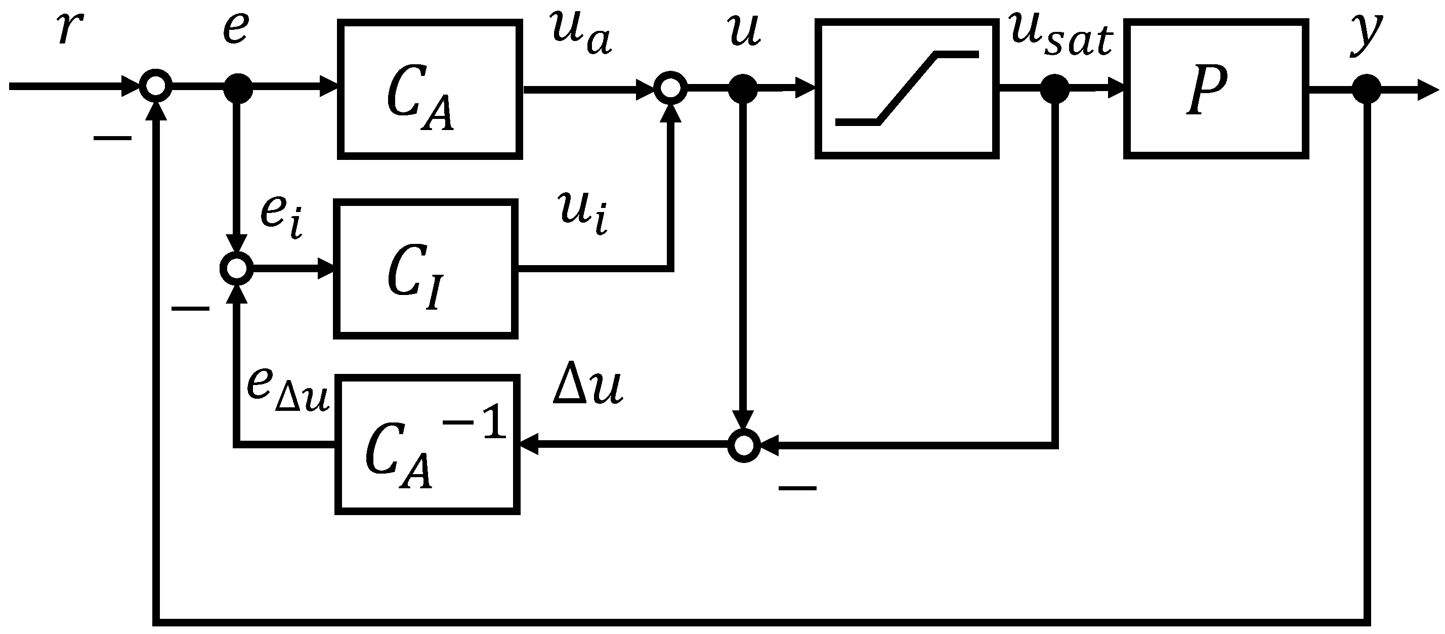
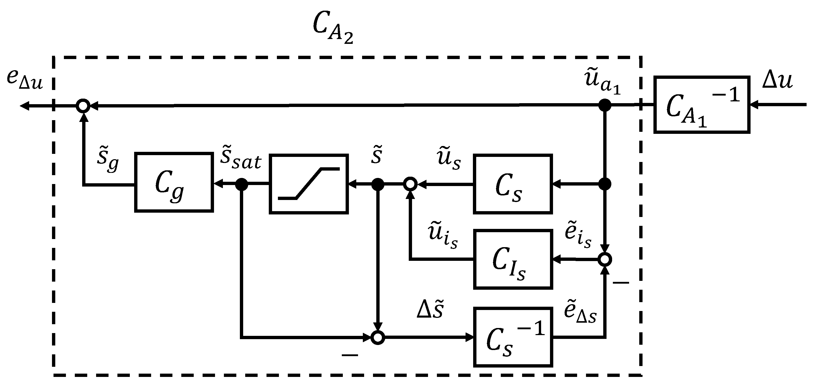
4.1. Nonlinear Back-Calculation Anti-Windup

The control system of the nonlinear back-calculation anti-windup is shown in Figure 2.

In Figure 2, the operators $C_{A_1}:W\to U,C_{A_2}:W\to W,C_A:W\to U$ are stable and invertible operators, the operator $C_1:W\to W$ is an invertible and monotonically increasing static operator, and it satisfies $C_1^{-1}\left(0\right)\left(t\right)=0$. The operator $C_2:W\to U$ is a stable operator, the operator $C_I$ is the same as in Equation (5), and the saturation operator $\sigma$ is defined as in Equation (6). In addition, the signal $u_f\left(t\right)\in U$ is also a bounded signal from an output feedback signal or a signal from other compensators. The behavior of the system upon saturation is analyzed during saturation. The input to the integrator $e_i\left(t\right)$ is expressed as

$$\begin{array}{cc}\hfill e_i\left(t\right)& =C_{A_2}\left(e\right)\left(t\right)-C_A^{-1}(\Delta u)\left(t\right),\hfill \end{array}$$

(12)

Therefore, the output of the controller $u_i\left(t\right)$ is expressed as

$$\begin{array}{cc}\hfill {\dot{u}}_i\left(t\right)=& k_I{C}_1\left(e_i\right)\left(t\right),\hfill \\ \hfill =& k_I{C}_1\left(C_{A_2}\left(e\right)\left(t\right)-C_A^{-1}(\Delta u)\left(t\right)\right),\hfill \\ \hfill =& k_I{C}_1\left(C_{A_2}\left(e\right)\left(t\right)-C_A^{-1}\left(C_{A_1}\left(e\right)\left(t\right)+u_{C_2}\left(t\right)+u_i\left(t\right)+u_f\left(t\right)-u_{sat}\left(t\right)\right)\right).\hfill \end{array}$$

(13)

To obtain the same result as in Equation (11), it is necessary that the following holds from Equation (13) when sufficient time has passed.

$$\begin{array}{c}\hfill \left\{\begin{array}{c}\underset{t\to \infty }{lim}\left(C_A{C}_{A_2}-C_{A_1}\right)\left(e\right)\left(t\right)=0\hfill \\ u_i\left(t\right){{|}_{t\to \infty }=\left(-u_{C_2}-u_f+u_{sat}\right)\left(t\right)|}_{t\to \infty }\hfill \end{array}\right..\end{array}$$

(14)

Note that from Equation (14), the operator $C_A$ must be designed to be $C_{A_1}{C}_{A_2}^{-1}$ when sufficient time has passed.

4.2. Application to Integral Sliding Mode Control

This section applies the nonlinear back-calculation anti-windup to ISMC. Integral sliding mode control is a control method that constrains the system state to a switching surface that includes an integrator [19,20,21]. For simplicity of discussion, the plant $P:U\to Y$ is represented as a tank system as:

$$\begin{array}{c}\hfill P\left(u\right)\left(t\right):\dot{y}\left(t\right)=-{\displaystyle \frac{a}{A}}\sqrt{2gy\left(t\right)}+{\displaystyle \frac{1}{A}}u\left(t\right),\end{array}$$

(15)

where the output $y\left(t\right)$ is the liquid level of the tank system, the control input $u\left(t\right)$ is the flow rate, A is the cross-sectional area of the tank, a is the cross-sectional area of the outlet, and g is the gravitational acceleration. Design the integral sliding mode controller $C:W\times Y\to U$. The switching surface $s:W\to W$ is defined as:

$$\begin{array}{c}\hfill s\left(t\right)=k_{P}e\left(t\right)+k_I{\int }_0^{t}e\left(\tau \right)d\tau +\dot{e}\left(t\right),\end{array}$$

(16)

where $k_P,k_I>0$ are design parameters. The controller $C:W\times Y\to U$ calculated from the switching surface is expressed as:

$$C\left(\begin{array}{c}r\\ y\end{array}\right)\left(t\right):\left\{\begin{array}{c}e\left(t\right)=r\left(t\right)-y\left(t\right)\hfill \\ s\left(t\right)=k_{P}e\left(t\right)+k_I{\int }_0^{t}e\left(\tau \right)d\tau +\dot{e}\left(t\right)\hfill \\ s_{sat}\left(t\right)=\mathrm{sgn}\left(s\right)\left(t\right)\hfill \\ u\left(t\right)=A\left(k_{P}e\left(t\right)+k_I{\int }_0^{t}e\left(\tau \right)d\tau +\dot{r}\left(t\right)+{\displaystyle \frac{a}{A}}\sqrt{2gy\left(t\right)}+\eta {\int }_0^t{s}_{sat}\left(\tau \right)d\tau \right)\hfill \end{array}\right.,$$

(17)

where, to suppress chattering, the sign function sgn is replaced with the saturation function ${\sigma }_s$:

$$\begin{array}{cc}\hfill & {\sigma }_s\left(s\right)\left(t\right):s_{sat}\left(t\right)=\left\{\begin{array}{cc}1\hfill & s\left(t\right)>1\hfill \\ s\left(t\right)\hfill & -1\le s\left(t\right)\le 1\hfill \\ -1\hfill & s\left(t\right)<-1\hfill \end{array}\right..\hfill \end{array}$$

(18)

Equation (17) is transformed as:

$$C\left(\begin{array}{c}r\\ y\end{array}\right)\left(t\right):\left\{\begin{array}{c}e\left(t\right)=r\left(t\right)-y\left(t\right)\hfill \\ s\left(t\right)=k_{P}e\left(t\right)+k_I{\int }_0^{t}e\left(\tau \right)d\tau +\dot{e}\left(t\right)\hfill \\ s_{sat}\left(t\right)={\sigma }_s\left(s\right)\left(t\right)\hfill \\ u\left(t\right)=A\left(k_{P}e\left(t\right)+\dot{r}\left(t\right)+{\displaystyle \frac{a}{A}}\sqrt{2gy\left(t\right)}+k_I{\int }_0^t\left(e\left(\tau \right)+{\displaystyle \frac{\eta }{k_I}}{s}_{sat}\left(\tau \right)\right)d\tau \right)\hfill \end{array}\right..$$

(19)

Since there are two types of saturation functions, one for the control input $u\left(t\right)$ and one for the nonlinear input term, it is necessary to consider anti-windup for each. Therefore, the integral sliding mode controller with nonlinear back-calculation anti-windup is shown in Figure 3, and each operator is expressed as:

$$\begin{array}{cc}\hfill & C_F\left(\begin{array}{c}r\\ y\end{array}\right)\left(t\right):u_f\left(t\right)=A\dot{r}\left(t\right)+a\sqrt{2gy\left(t\right)},\hfill \end{array}$$

(20)

$$\begin{array}{cc}\hfill & C_{A_1}\left(e\right)\left(t\right):u_{a_1}\left(t\right)=k_{P}e\left(t\right),\hfill \end{array}$$

(21)

$$\begin{array}{cc}\hfill & C_S\left(e\right)\left(t\right):u_s\left(t\right)=k_{P}e\left(t\right)+\dot{e}\left(t\right),\hfill \end{array}$$

(22)

$$\begin{array}{cc}\hfill & C_g\left(s_{sat}\right)\left(t\right):s_g\left(t\right)={\displaystyle \frac{\eta }{k_I}}{s}_{sat}\left(t\right),\hfill \end{array}$$

(23)

$$\begin{array}{cc}\hfill & C_{I_s}\left(e_{i_s}\right)\left(t\right):u_{i_s}\left(t\right)=k_I{\int }_0^t{e}_{i_s}\left(\tau \right)d\tau ,\hfill \end{array}$$

(24)

$$\begin{array}{cc}\hfill & C_I\left(e_i\right)\left(t\right):u_i\left(t\right)=k_I{\int }_0^t{e}_i\left(\tau \right)d\tau ,\hfill \end{array}$$

(25)

$$\begin{array}{cc}\hfill & \underset{t\to \infty }{lim}\left(C_s\left(e_{\Delta s}\right)-C_s\left(e\right)\right)\left(t\right)=0,\hfill \end{array}$$

(26)

$$\begin{array}{cc}\hfill & \underset{t\to \infty }{lim}\left(C_A{C}_{A_2}-C_{A_1}\right)\left(e\right)\left(t\right)=0,\hfill \end{array}$$

(27)

where the operator $C_A$ requires anti-windup compensation, as shown in Figure 4, because the operator $C_{A_2}$ exists, as indicated by Equation (27). When sufficient time has passed, the outputs of each integrator are expressed as:

$$\begin{array}{c}\hfill \left\{\begin{array}{c}{u}_{i_s}\left(t\right){{|}_{t\to \infty }=s_{sat}\left(t\right)|}_{t\to \infty }\hfill \\ u_i\left(t\right){{|}_{t\to \infty }=\left(-a\sqrt{2gy\left(t\right)}+u_{sat}\left(t\right)\right)|}_{t\to \infty }=0\hfill \\ {\tilde{u}}_{i_s}\left(t\right){{|}_{t\to \infty }={\tilde{s}}_{sat}\left(t\right)|}_{t\to \infty }\hfill \end{array}\right..\end{array}$$

(28)

The stability of the designed control system is proven. First, the stability in the non-saturated state is proven. The function $V\left(t\right)$ is defined as:

$$\begin{array}{c}\hfill V\left(t\right)={\displaystyle \frac{1}{2}}{s}^2\left(t\right).\end{array}$$

(29)

In Equation (17), the function $f_s\left(t\right)$ is defined as:

$$\begin{array}{c}\hfill f_s\left(t\right)=k_{P}e\left(t\right)+k_I{\int }_0^{t}e\left(\tau \right)d\tau .\end{array}$$

(30)

Differentiating the function $V\left(t\right)$, we obtain:

$$\begin{array}{cc}\hfill \dot{V}\left(t\right)& =s\left(t\right)\dot{s}\left(t\right),\hfill \\ \hfill & =s\left(t\right)\left({\displaystyle \frac{d}{dt}}{f}_s\left(t\right)+\left(\ddot{r}\left(t\right)-\ddot{y}\left(t\right)\right)\right),\hfill \\ \hfill & =s\left(t\right)\left({\displaystyle \frac{d}{dt}}{f}_s\left(t\right)+\ddot{r}\left(t\right)-{\displaystyle \frac{d}{dt}}\left(-{\displaystyle \frac{a}{A}}\sqrt{2gy\left(t\right)}+{\displaystyle \frac{1}{A}}u\left(t\right)\right)\right),\hfill \\ \hfill & =s\left(t\right)({\displaystyle \frac{d}{dt}}{f}_s\left(t\right)+\ddot{r}\left(t\right)-{\displaystyle \frac{d}{dt}}(-{\displaystyle \frac{a}{A}}\sqrt{2gy\left(t\right)}+f_s\left(t\right)+\dot{r}\left(t\right)+{\displaystyle \frac{a}{A}}\sqrt{2gy\left(t\right)}\hfill \\ \hfill & +\eta {\int }_0^t{s}_{sat}\left(\tau \right)d\tau \left)\right),\hfill \\ \hfill & =-\eta s\left(t\right)\mathrm{sgn}\left(s\left(t\right)\right),\hfill \\ \hfill & <0.\hfill \end{array}$$

(31)

Therefore, the sliding condition is satisfied in the non-saturated state. Next, the stability in the saturated state is proven. In the saturated state, the control input $u_{sat}$ is $\overline{u}$ or $\underline{u}$, and the system is stable because the plant is stable. Therefore, the stability of the control system is guaranteed.

4.3. Application to Right Coprime Factorization

This section applies the nonlinear back-calculation anti-windup to RCF. Right coprime factorization is a method that guarantees BIBO stability for a given reference input [16,22]. The mathematical model is given by Equation (15). The control system is designed using RCF in the unsaturated case. The right factorization of the plant P is expressed as

$$\begin{array}{cc}\hfill & N_R\left({\omega }_r\right)\left(t\right):\left\{\begin{array}{c}e\left(t\right)={\omega }_r\left(t\right)-y\left(t\right)\hfill \\ {\dot{e}}_i\left(t\right)=e\left(t\right)\hfill \\ \dot{y}\left(t\right)={\displaystyle \frac{k_P}{A}}\sqrt{|{\omega }_r\left(t\right)-y\left(t\right)|}\mathrm{sgn}({\omega }_r\left(t\right)-y\left(t\right))+{\displaystyle \frac{k_I}{A}}{e}_i\left(t\right)\hfill \end{array}\right.,\hfill \end{array}$$

(32)

$$\begin{array}{cc}\hfill & D_R\left({\omega }_r\right)\left(t\right):\left\{\begin{array}{c}e\left(t\right)={\omega }_r\left(t\right)-y\left(t\right)\hfill \\ {\dot{e}}_i\left(t\right)=e\left(t\right)\hfill \\ \dot{y}\left(t\right)={\displaystyle \frac{k_P}{A}}\sqrt{|{\omega }_r\left(t\right)-y\left(t\right)|}\mathrm{sgn}({\omega }_r\left(t\right)-y\left(t\right))+{\displaystyle \frac{k_I}{A}}{e}_i\left(t\right)\hfill \\ u\left(t\right)=k_P\sqrt{|{\omega }_r\left(t\right)-y\left(t\right)|}\mathrm{sgn}({\omega }_r\left(t\right)-y\left(t\right))+a\sqrt{2gy\left(t\right)}+k_I{e}_i\left(t\right)\hfill \end{array}\right.,\hfill \end{array}$$

(33)

where $k_P,k_I>0$ are design parameters. The controller C is expressed as:

$$C\left(\begin{array}{c}r\\ y\end{array}\right)\left(t\right):\left\{\begin{array}{c}e\left(t\right)=r\left(t\right)-y\left(t\right)\hfill \\ {\dot{e}}_i\left(t\right)=e\left(t\right)\hfill \\ u\left(t\right)=k_P\sqrt{\left|e\right(t\left)\right|}\mathrm{sgn}\left(e\left(t\right)\right)+a\sqrt{2gy\left(t\right)}+k_I{e}_i\left(t\right)\hfill \end{array}\right..$$

(34)

Additionally, to suppress chattering, the sign function sgn is approximated by the saturation function represented in Equation (18). The controller C with nonlinear back-calculation anti-windup is shown in Figure 5, and each operator is expressed as:

$$\begin{array}{cc}\hfill & C_F\left(y\right)\left(t\right):u_f\left(t\right)=a\sqrt{2gy\left(t\right)},\hfill \end{array}$$

(35)

$$\begin{array}{cc}\hfill & C_{A_1}\left(e\right)\left(t\right):u_{a_1}\left(t\right)=k_P\sqrt{\left|e\right(t\left)\right|}\mathrm{sat}\left(e\left(t\right)\right),\hfill \end{array}$$

(36)

$$\begin{array}{cc}\hfill & C_I\left(e_i\right)\left(t\right):u_i\left(t\right)=k_I{\int }_0^t{e}_i\left(\tau \right)d\tau ,\hfill \end{array}$$

(37)

$$\begin{array}{cc}\hfill & \underset{t\to \infty }{lim}\left(C_A\left(e_{\Delta u}\right)-C_{A_1}\left(e\right)\right)\left(t\right)=0.\hfill \end{array}$$

(38)

When sufficient time has passed, the outputs of each integrator are expressed as:

$$\begin{array}{c}\hfill u_i\left(t\right){{|}_{t\to \infty }=\left(-a\sqrt{2gy\left(t\right)}+u_{sat}\left(t\right)\right)|}_{t\to \infty }=0.\end{array}$$

(39)

The stability of the designed control system is proven. First, the stability in the non-saturated state is proven. In Equation (34), the function $f_c\left(t\right)$ is defined as:

$$\begin{array}{c}\hfill f_c\left(t\right)=a\sqrt{2gy\left(t\right)}+k_I{e}_i\left(t\right).\end{array}$$

(40)

Substituting Equations (32)–(34) into the generalized Bézout identity, we obtain:

$$\begin{array}{cc}\hfill C^{†}\left(\begin{array}{c}{N}_R\\ D_R\end{array}\right)\left({\omega }_r\right)\left(t\right)& ={\left({\displaystyle \frac{1}{k_P}}\left(u\left(t\right)-f_c\left(t\right)\right)\right)}^2\mathrm{sgn}\left(u\left(t\right)-f_c\left(t\right)\right)+y\left(t\right),\hfill \\ \hfill & =\left({\omega }_r\left(t\right)-y\left(t\right)\right)\mathrm{sgn}\left({\omega }_r\left(t\right)-y\left(t\right)\right)+y\left(t\right),\hfill \\ \hfill & ={\omega }_r\left(t\right).\hfill \end{array}$$

(41)

Therefore, the generalized Bézout identity is satisfied in the non-saturated state. Next, the stability in the saturated state is proven. In the saturated state, the control input $u_{sat}\left(t\right)$ is $\overline{u}$ or $\underline{u}$, and the system is stable because the plant is stable. Therefore, the stability of the control system is guaranteed.

5. Simulations

Simulations of liquid level control in a tank system using nonlinear back-calculation anti-windup applied to ISMC and RCF are performed. Additionally, each result is compared with conditional integration. This paper prevents the integrator from increasing when the input is saturated.

5.1. Simulations of Integral Sliding Mode Control

Simulations are performed using the control system designed in the previous section with Python. The simulation parameters are shown in

Table 1. Simulation parameters of ISMC.

Symbol	Quantity	Value
A	Cross-sectional area of the tank	1 m2
a	Cross-sectional area of the outlet	$0.1$ m2
g	Acceleration due to gravity	$9.8$ m/s2
$T_s$	Sampling period	1 s
$\overline{u}$	Upper limit of the input	$1.2$ m3/s
$\underline{u}$	Lower limit of the input	0 m3/s
$k_P$	Design parameter of ISMC	1.5
$k_I$	Design parameter of ISMC	$0.1$
$\eta$	Design parameter of ISMC	$0.1$

.

Various step signals of different magnitudes are applied for $T=1500\mathrm{s}$. However, during the period from 500 to 750 s, a value that cannot reach the reference input due to input constraints is applied. Additionally, the results are evaluated not only with graphs but also using Root Mean Squared Error (RMSE) and Mean Absolute Error (MAE). RMSE and MAE are defined as follows:

$$\begin{array}{cc}\hfill & \mathrm{RMSE}=\sqrt{{\displaystyle \frac{1}{N}}\sum _{i=1}^N{\left(e\left(i\right)\right)}^2},\hfill \end{array}$$

(42)

$$\begin{array}{cc}\hfill & \mathrm{MAE}={\displaystyle \frac{1}{N}}\sum _{i=1}^N\left|e\left(i\right)\right|,\hfill \end{array}$$

(43)

where $N=T/T_s$.

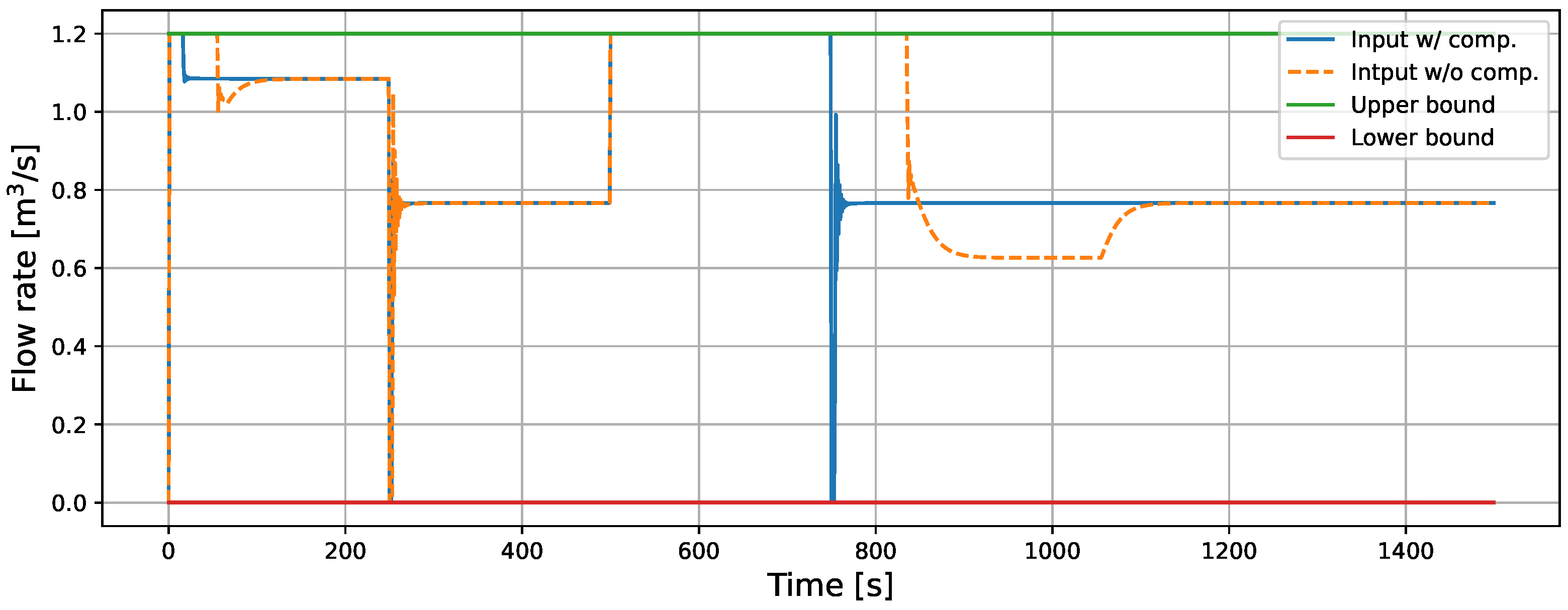
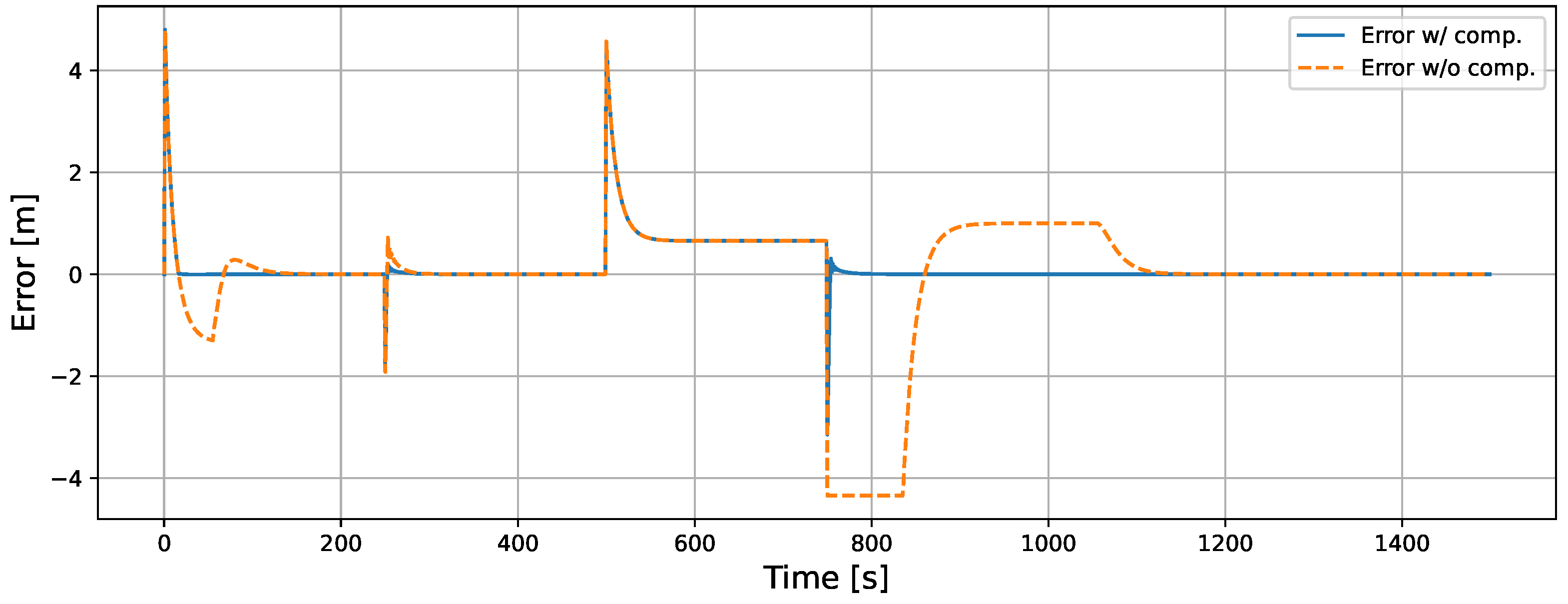
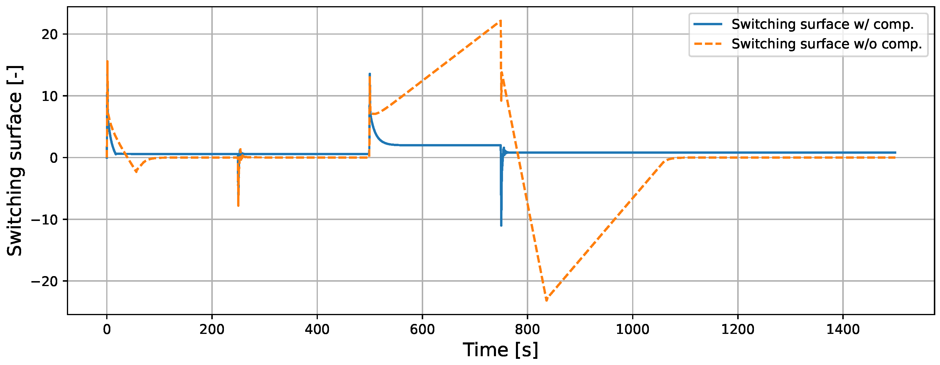
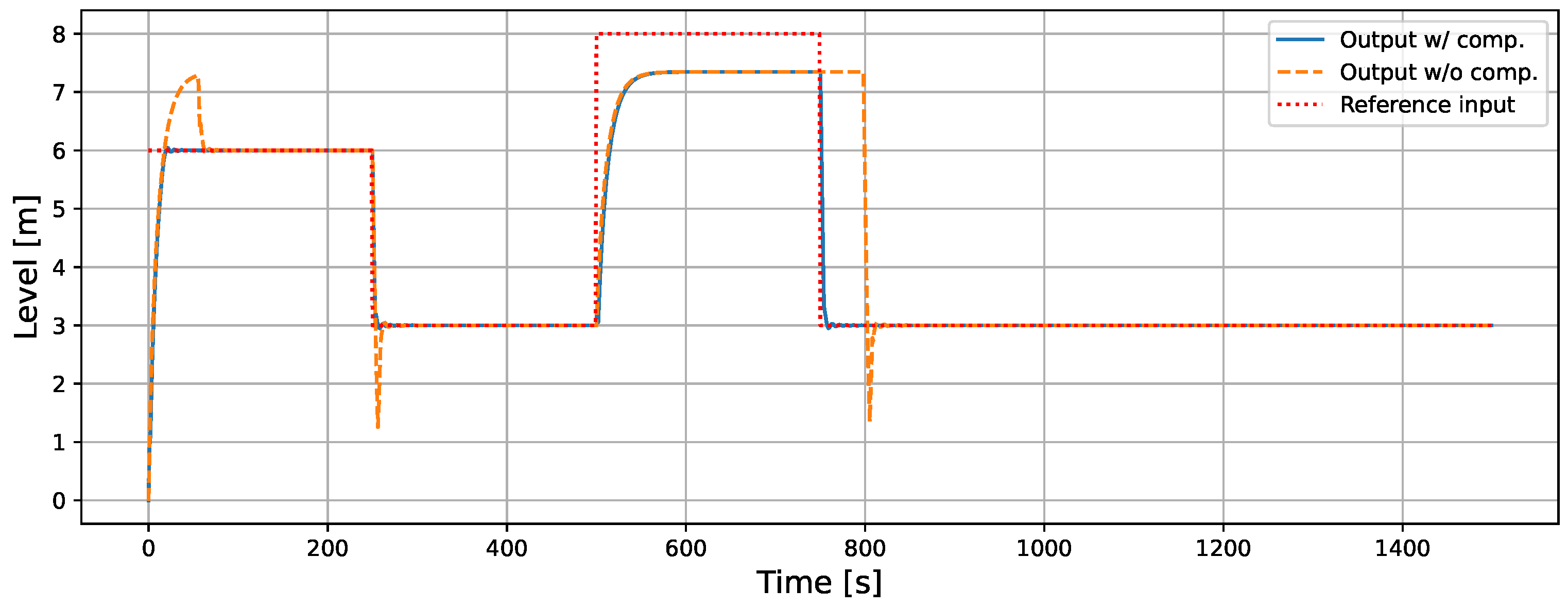
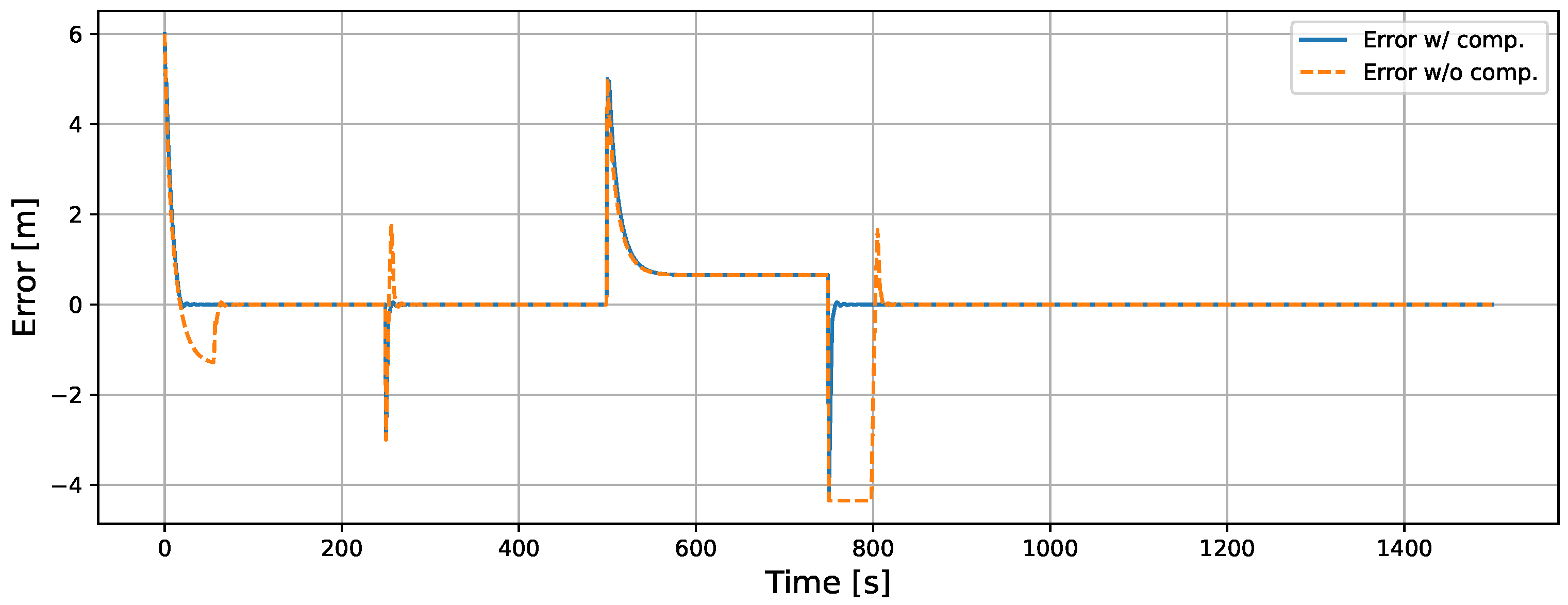
5.1.1. Comparison with and Without the Proposed Method in ISMC

The simulation results with and without the proposed method are shown in Figure 6, Figure 7, Figure 8, Figure 9, Figure 10 and Figure 11 and

Table 2. RMSE and MAE with and without anti-windup compensator in ISMC.

	With Compensator	Without Compensator
RMSE [m]	0.49	1.23
MAE [m]	0.17	0.61

. From Figure 6 and Figure 8, it can be observed that without compensation, significant overshoot occurs during changes in the reference input, whereas with compensation, this is mitigated, resulting in improved tracking accuracy. This trend is particularly evident in the intervals 0–150 s and 750–1100 s. This phenomenon occurs because, during input saturation, changes in the integral state are not immediately reflected in the input, causing the integral state to increase excessively and prolong the saturation state. In the proposed method, excessive components of the integral state are promptly removed during saturation, allowing the saturation state to end at an appropriate time, thereby minimizing overshoot. This is supported by Figure 7, Figure 10, and Figure 11, where, in the intervals 0–150 s and 750–1100 s, the integral state decreases immediately with compensation, whereas without compensation, the integral state continues to increase leisurely, resulting in prolonged input saturation. This phenomenon is particularly pronounced in these intervals simply because the changes in the reference input are larger during these periods.

Interestingly, a notable feature of this result is that in the interval 850–1100 s, the liquid level does not track the reference value despite the input not being saturated. This phenomenon occurs because, although the control input is not saturated, the nonlinear input is saturated. ISMC has two terms where saturation and integrators exist: the control input and the nonlinear input. Windup can occur if either is saturated. From Figure 11, it can be confirmed that during the relevant interval, the integral state of the control input (orange) converges to a constant value, whereas the integral state of the nonlinear input (blue) experiences windup and converges simultaneously with the liquid level. Even in such complex scenarios, the proposed method stabilizes each integral state independently, enabling the system to promptly track the reference value. These effects lead to the improvement of RMSE and MAE, as shown in Table 2.

Additionally, when an unreachable step signal of 8 m is applied, the output of the integrator, as shown in Figure 10, eventually matches the condition described in Equation (28). From this result, it is shown that the theorem regarding the convergence of the integral state in the proposed method is correct. Note that in Figure 9, the switching surface is not at zero due to the influence of the integral term of the ISMC.

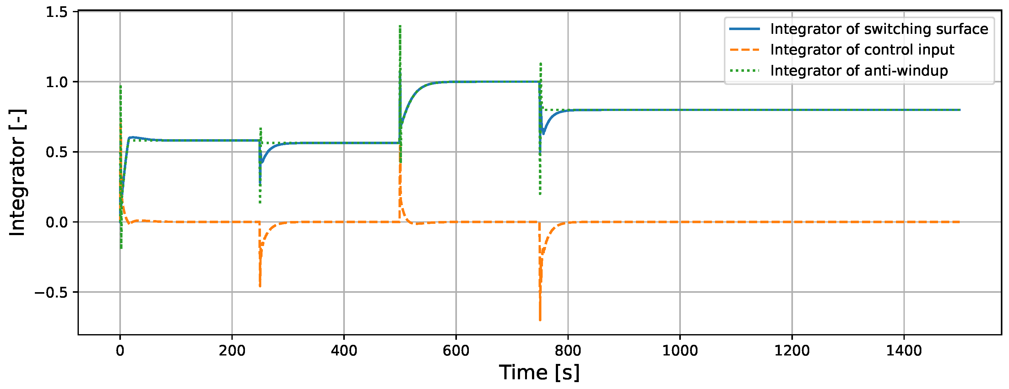
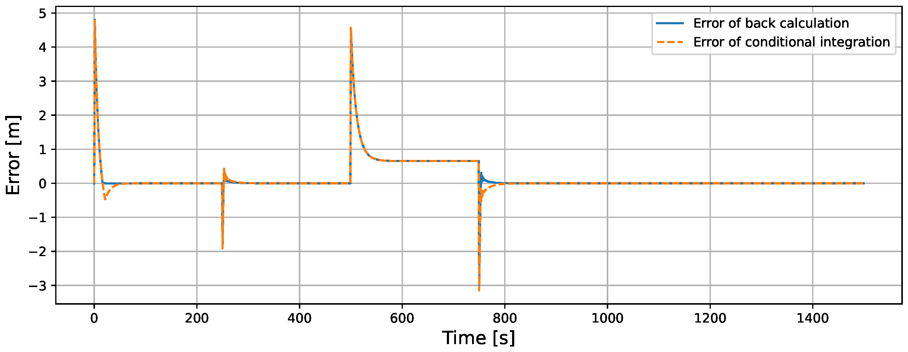
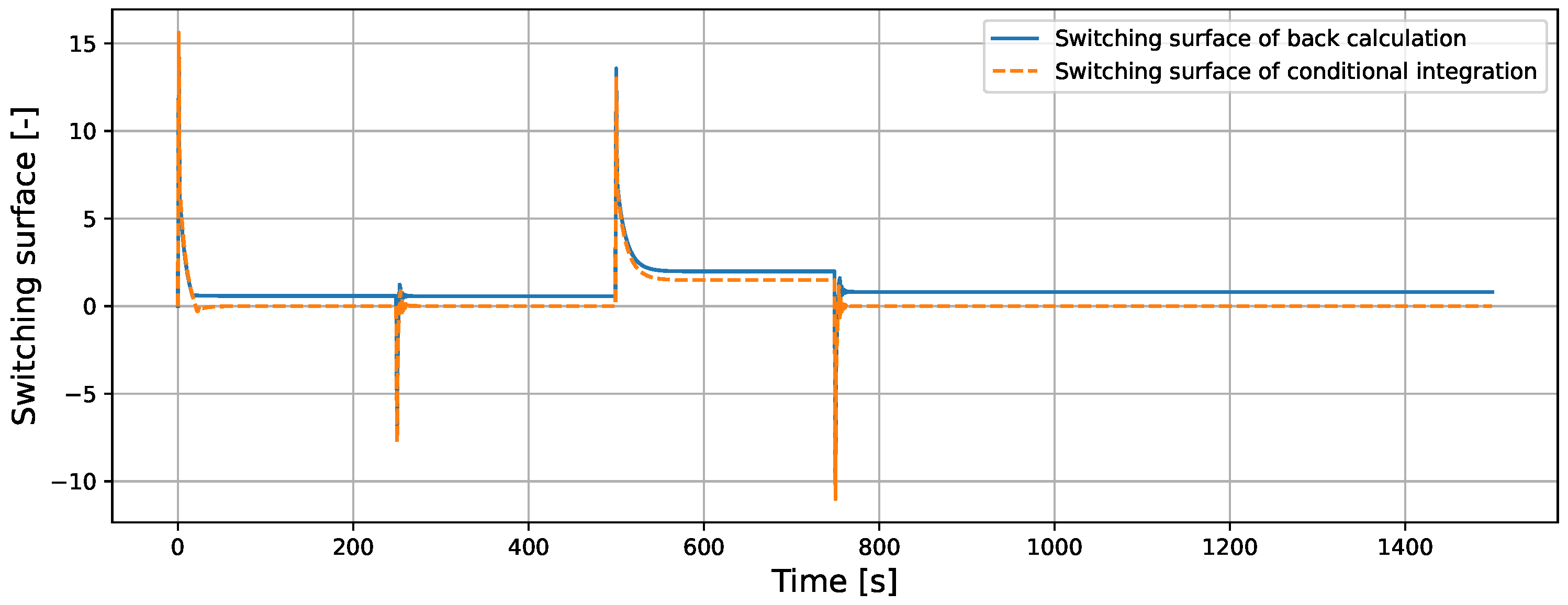
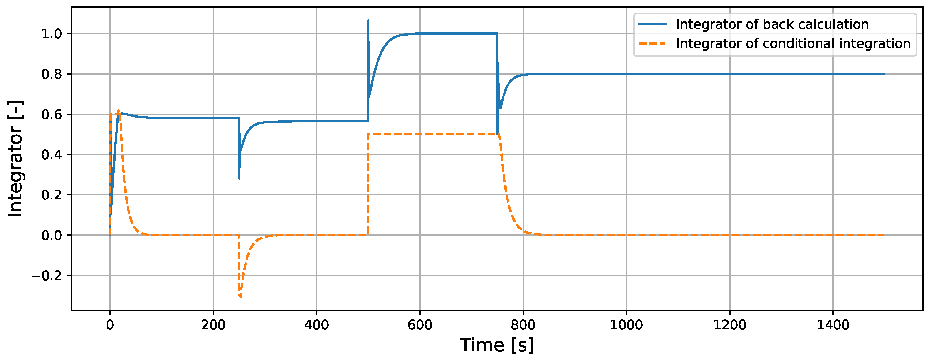
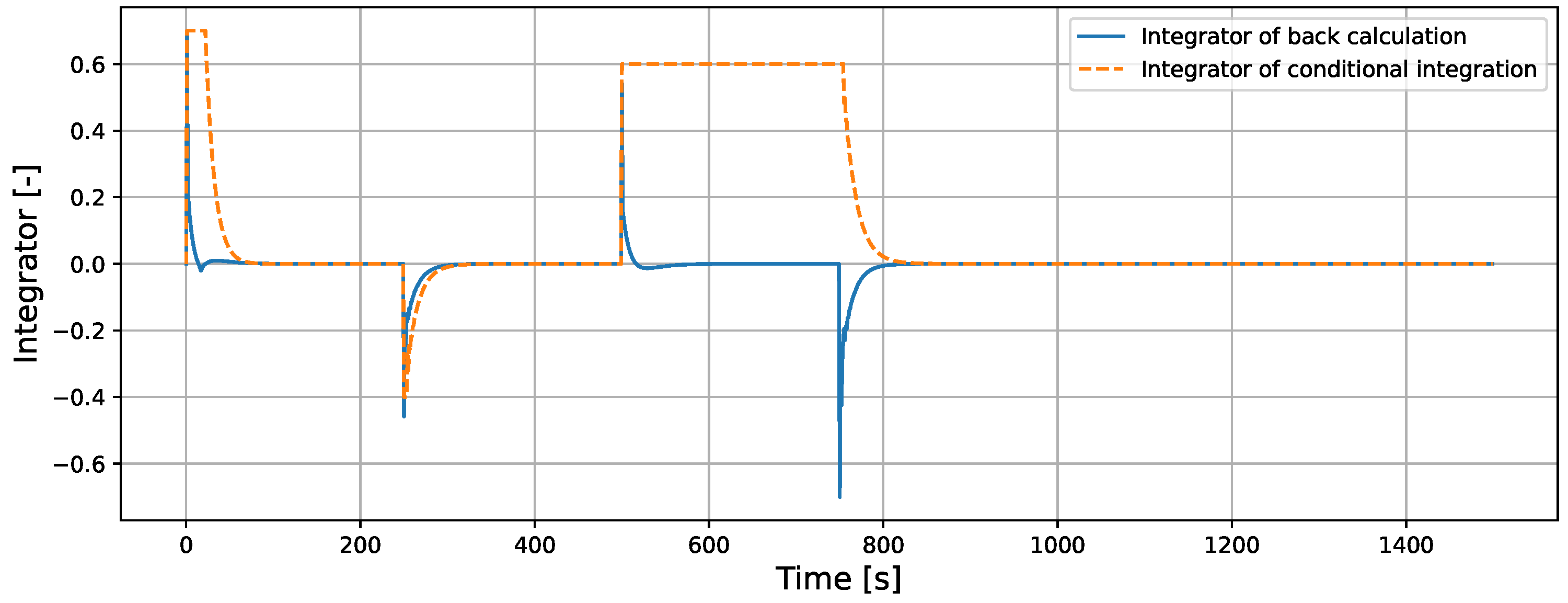
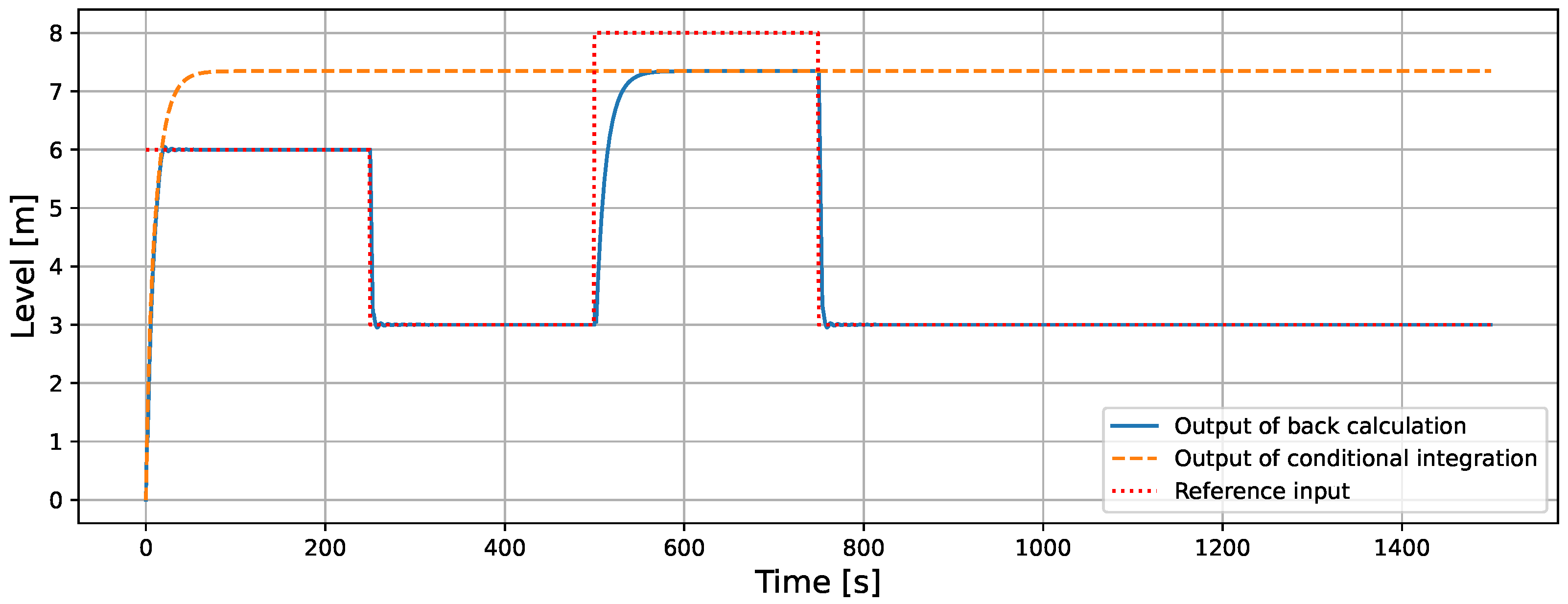
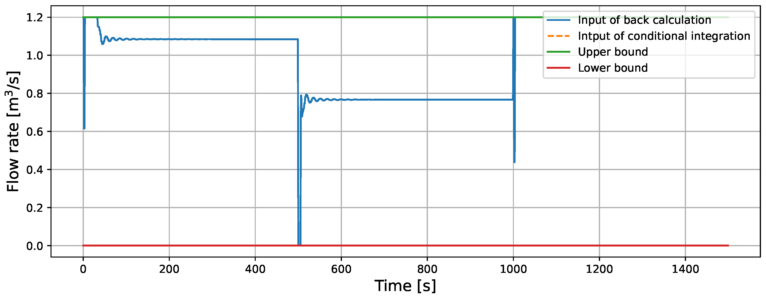
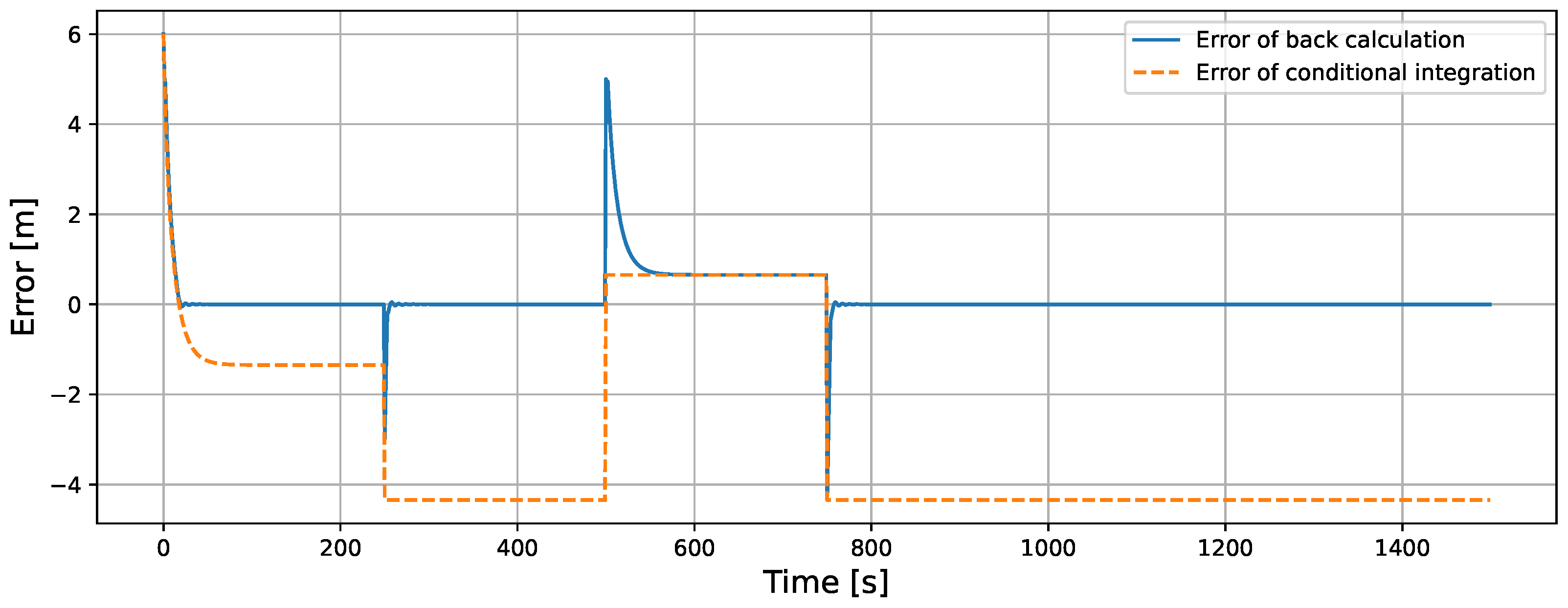
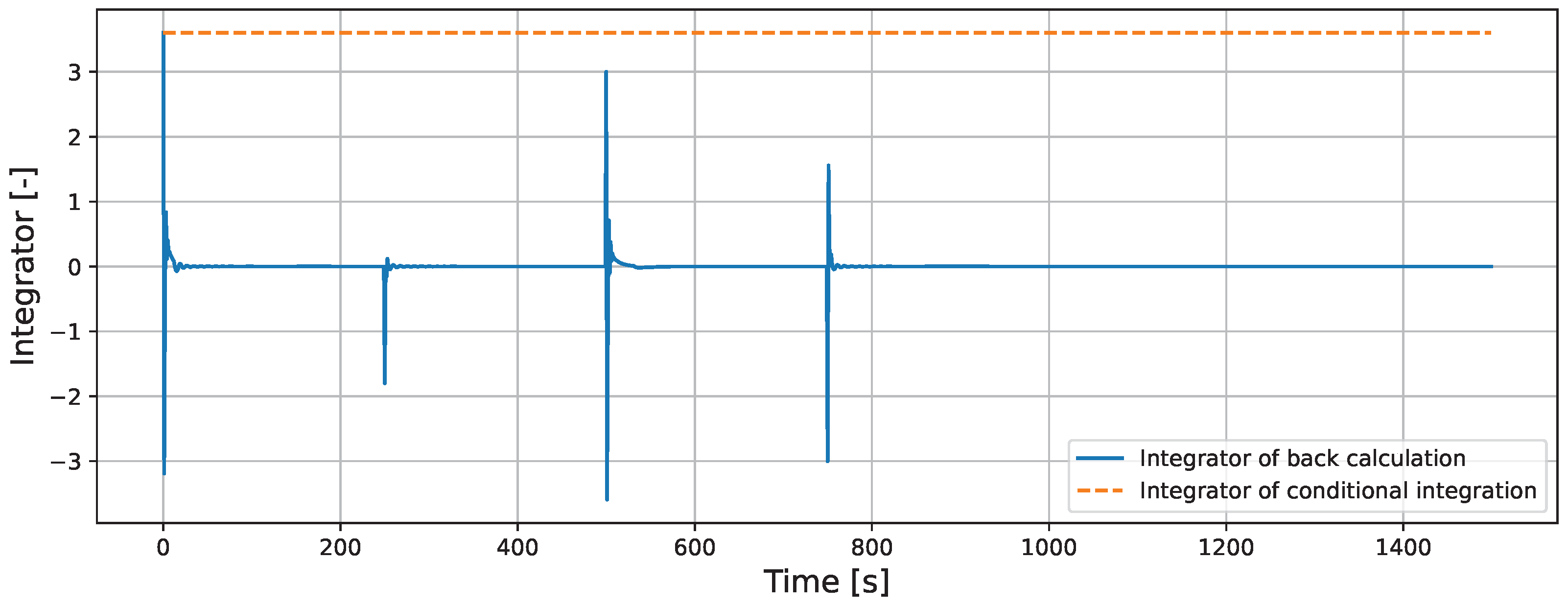
5.1.2. Comparison of Back-Calculation and Conditional Integration in ISMC

The simulation results comparing back-calculation and conditional integration are shown in Figure 12, Figure 13, Figure 14, Figure 15, Figure 16 and Figure 17 and

Table 3. RMSE and MAE of back-calculation and conditional integration in ISMC.

	Back-Calculation	Conditional Integration
RMSE [m]	0.486	0.488
MAE [m]	0.166	0.173

. From Figure 12 and Figure 14, it can be observed that when a step signal of 6 m is applied, back-calculation does not exhibit overshoot, whereas conditional integration does. This is because, as shown in Figure 16 and Figure 17, the integrator decreases during saturation in back-calculation, while it remains unchanged in conditional integration. Furthermore, when the reference input changes to 3 m, back-calculation does not exhibit undershoot, while conditional integration does. When an unreachable step signal of 8 m is applied, it can be seen from Figure 16 and Figure 17 that the integrator in back-calculation converges to the saturated value, whereas the integrator in conditional integration does not converge. This behavior is likely due to conditional integration halting the integrator during saturation. Moreover, when the reference input changes from 8 m to 3 m, back-calculation exhibits undershoot, while conditional integration does not. This is likely because, as shown in Figure 17, the integrator in back-calculation increases more than in conditional integration during the reference input change. Figure 16 confirms that conditional integration exhibits oscillations. Finally, the RMSE and MAE of back-calculation and conditional integration are shown in Table 3. There exists a slight difference in RMSE and MAE, but this is due to the error being maintained for a long time when an unreachable reference input is applied. This difference is considered significant enough to be relevant, even if it is only in the third decimal place.

5.2. Simulations of Right Coprime Factorization

Simulations are performed using the control system designed in the previous section. The parameters of the mathematical model and the sampling period are the same as in Table 1, and the design parameters of the RCF are $k_P=1.5,k_I=0.6$.

5.2.1. Comparison with and Without Anti-Windup Compensator in RCF

The simulation results under the same conditions as in Section 5.1 are shown in Figure 18, Figure 19, Figure 20 and Figure 21 and

Table 4. RMSE and MAE with and without anti-windup compensator in RCF.

	With Compensator	Without Compensator
RMSE [m]	0.59	0.98
MAE [m]	0.19	0.35

. From Figure 18, Figure 19, Figure 20 and Figure 21, results similar to those of ISMC were obtained for RCF. Additionally, when an unreachable reference input is applied and sufficient time has passed, it can be confirmed that the value of the integrator with the anti-windup compensator in Figure 21 matches (39). It can be observed that Figure 19 exhibits oscillations when the reference input changes, which is due to the influence of the saturation function.

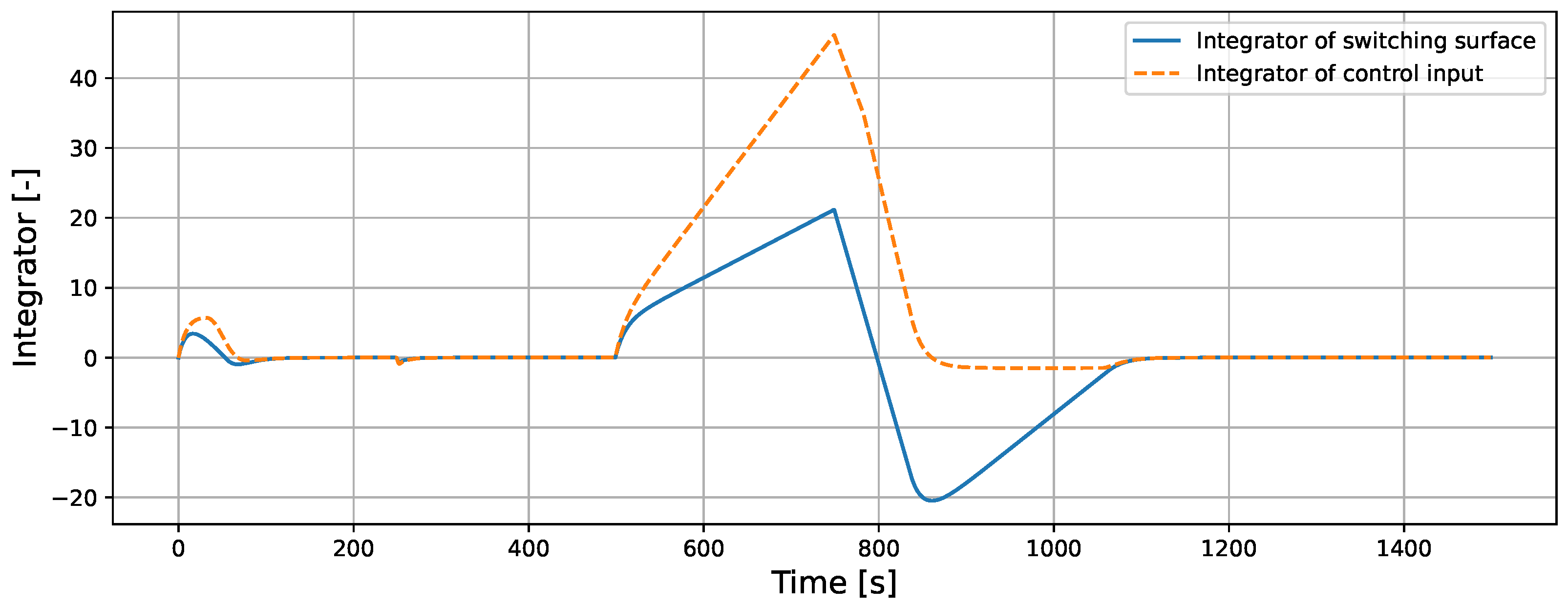
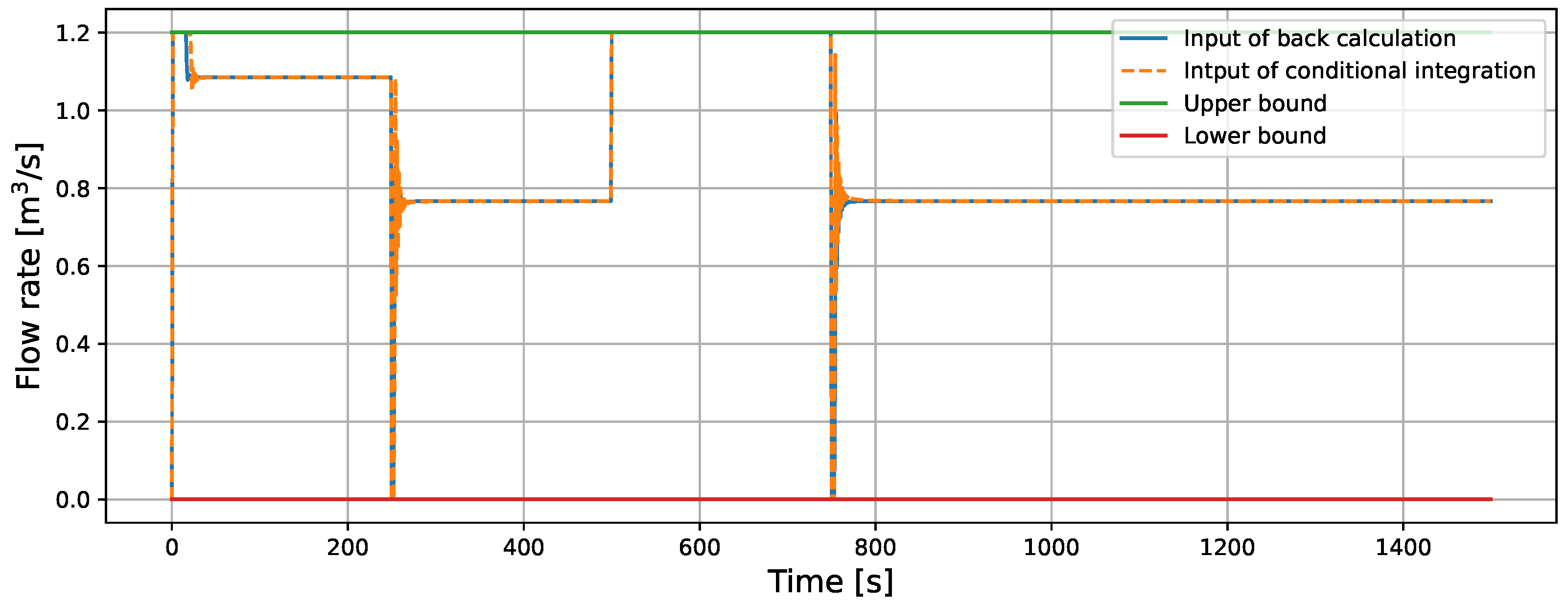
5.2.2. Comparison of Back-Calculation and Conditional Integration in RCF

The simulation results comparing back-calculation and conditional integration are shown in Figure 22, Figure 23, Figure 24 and Figure 25 and

Table 5. RMSE and MAE of back-calculation and conditional integration in RCF.

	Back-Calculation	Conditional Integration
RMSE [m]	0.59	3.61
MAE [m]	0.19	3.23

. Looking at Figure 22, this result shows a significant difference from other results, where the output in the conditional integration method remains stuck at the maximum achievable value. This is because, as seen in Figure 25, the integral state is fixed at a very large value of $3.3{\mathrm{m}}^3/\mathrm{s}$. Even when all inputs other than the integral are summed, they cannot reach $3.3{\mathrm{m}}^3/\mathrm{s}$, causing the control input to be saturated solely by the integral state. As a result, the integral state is not updated. In other words, this phenomenon is caused by the halting of the integral state update, which does not occur with the proposed method that does not involve stopping the integral. In this regard, the proposed method is clearly superior.

6. Conclusions

This paper proposes a method of back-calculation anti-windup for nonlinear controllers. The proposed method is applicable to stable plants and is a natural extension of the back-calculation anti-windup method for linear controllers. Simulations of liquid level control in a tank system using the proposed method with ISMC and RCF showed that the system response is faster than without the anti-windup compensator. Additionally, the results of RCF demonstrated that the proposed method outperforms conditional integration. In the future, we intend to extend this method to be applicable to more complex systems.

References

1. Markaroglu, H.; Guzelkaya, M.; Eksin, I.; Yesil, E. Tracking time adjustment in back calculation anti-windup scheme. In Proceedings of the 20th European Conference on Modelling and Simulation, Bonn, Germany, 28–31 May 2006. [Google Scholar]
2. Åström, K.J.; Hägglund, T. The future of PID control. Control Eng. Pract. 2001, 9, 1163–1175. [Google Scholar] [CrossRef]
3. Ang, K.H.; Chong, G.; Li, Y. PID control system analysis, design, and technology. IEEE Trans. Control Syst. Technol. 2005, 13, 559–576. [Google Scholar]
4. Iqbal, J.; Ullah, M.; Khan, S.G.; Khelifa, B.; Ćuković, S. Nonlinear control systems-A brief overview of historical and recent advances. Nonlinear Eng. 2017, 6, 301–312. [Google Scholar] [CrossRef]
5. Lin, Z.; Stoorvogel, A.A.; Saberi, A. Output regulation for linear systems subject to input saturation. Automatica 1996, 32, 29–47. [Google Scholar] [CrossRef]
6. Hu, T.; Lin, Z. Control Systems with Actuator Saturation: Analysis and Design; Springer Science & Business Media: Berlin, Germany, 2001. [Google Scholar]
7. Tarbouriech, S.; Turner, M. Anti-windup design: An overview of some recent advances and open problems. IET Control Theory Appl. 2009, 3, 1–19. [Google Scholar] [CrossRef]
8. García, C.E.; Prett, D.M.; Morari, M. Model predictive control: Theory and practice—A survey. Automatica 1989, 25, 335–348. [Google Scholar] [CrossRef]
9. Fertik, H.A.; Ross, C.W. Direct digital control algorithm with anti-windup feature. ISA Trans. 1967, 6, 317–328. [Google Scholar]
10. Rachev, E.; Petrov, V. Integral anti-windup correction in PI current controllers for electrical drives. In Proceedings of the 2020 12th Electrical Engineering Faculty Conference (BulEF), Varna, Bulgaria, 9–12 September 2020; IEEE: Piscataway, NJ, USA, 2020; pp. 1–4. [Google Scholar]
11. Rundqwist, L. Anti-reset Windup for PID Controllers. IFAC Proc. Vol. 1990, 23, 453–458. [Google Scholar] [CrossRef]
12. Gallun, S.E.; Matthews, C.W.; Senyard, C.P.; Slater, B. Windup protection and initialization for advanced digital control. Hydrocarb. Process. 1985, 67, 63–68. [Google Scholar]
13. Phelan, R. Automatic Control Systems; Cornell Univ. Press: Ithaca, NY, USA, 1977. [Google Scholar]
14. Deng, M.; Inoue, A.; Yanou, A.; Hirashima, Y. Continuous-time anti-windup generalized predictive control of non-minimum phase processes with input constraints. In Proceedings of the 42nd IEEE International Conference on Decision and Control (IEEE Cat. No.03CH37475), Maui, HI, USA, 9–12 December 2003; Volume 5, pp. 4457–4462. [Google Scholar]
15. De Figueiredo, R.J.; Chen, G. Nonlinear Feedback Control Systems: An Operator Theory Approach; Academic Press: Cambridge, MA, USA, 1993. [Google Scholar]
16. Deng, M. Operator-Based Nonlinear Control Systems: Design and Applications; John Wiley & Sons: Hoboken, NJ, USA, 2014. [Google Scholar]
17. Bu, N.; Zhang, Y.; Zhang, Y.; Morohoshi, Y.; Deng, M. Robust Control for Hysteretic Microhand Actuator Using Robust Right Coprime Factorization. IEEE Trans. Autom. Control 2024, 69, 3982–3988. [Google Scholar] [CrossRef]
18. Jin, G.; Deng, M. Operator-based robust nonlinear free vibration control of a flexible plate with unknown input nonlinearity. IEEE/CAA J. Autom. Sin. 2020, 7, 442–450. [Google Scholar] [CrossRef]
19. Young, K.D.; Utkin, V.I.; Ozguner, U. A control engineer’s guide to sliding mode control. IEEE Trans. Control Syst. Technol. 1999, 7, 328–342. [Google Scholar] [CrossRef]
20. Yu, X.; Feng, Y.; Man, Z. Terminal Sliding Mode Control – An Overview. IEEE Open J. Ind. Electron. Soc. 2021, 2, 36–52. [Google Scholar] [CrossRef]
21. Niu, Y.; W C Ho, D.; Lam, J. Robust integral sliding mode control for uncertain stochastic systems with time-varying delay. Automatica 2005, 41, 873–880. [Google Scholar] [CrossRef]
22. Baños, A. Stabilization of nonlinear systems based on a generalized Bezout identity. Automatica 1996, 32, 591–595. [Google Scholar] [CrossRef]
Figure 1. PI controller with anti-windup.
Processes 13 01266 g001
Figure 2. Nonlinear back-calculation anti-windup.
Processes 13 01266 g002
Figure 3. ISMC with back-calculation anti-windup scheme.
Processes 13 01266 g003
Figure 4. Operator C A 1 .
Processes 13 01266 g004
Figure 5. RCF with back-calculation anti-windup scheme.
Processes 13 01266 g005
Figure 6. Level of ISMC.
Processes 13 01266 g006
Figure 7. Flow rate of ISMC.
Processes 13 01266 g007
Figure 8. Error of ISMC.
Processes 13 01266 g008
Figure 9. Switching surface of ISMC.
Processes 13 01266 g009
Figure 10. Outputs of the integrators of ISMC (w/ comp.).
Processes 13 01266 g010
Figure 11. Outputs of the integrators of ISMC (w/o comp.).
Processes 13 01266 g011
Figure 12. Level of back-calculation and conditional integration in ISMC.
Processes 13 01266 g012
Figure 13. Flow rate of back-calculation and conditional integration in ISMC.
Processes 13 01266 g013
Figure 14. Error of back-calculation and conditional integration in ISMC.
Processes 13 01266 g014
Figure 15. Switching surface of back-calculation and conditional integration in ISMC.
Processes 13 01266 g015
Figure 16. Outputs of the switching surface’s integrators of back-calculation and conditional integration in ISMC.
Processes 13 01266 g016
Figure 17. Outputs of the control input’s integrators of back-calculation and conditional integration in ISMC.
Processes 13 01266 g017
Figure 18. Level of RCF.
Processes 13 01266 g018
Figure 19. Flow rate of RCF.
Processes 13 01266 g019
Figure 20. Error of RCF.
Processes 13 01266 g020
Figure 21. Output of the integrators of RCF.
Processes 13 01266 g021
Figure 22. Level of back-calculation and conditional integration in RCF.
Processes 13 01266 g022
Figure 23. Flow rate of back-calculation and conditional integration in RCF.
Processes 13 01266 g023
Figure 24. Error of back-calculation and conditional integration in RCF.
Processes 13 01266 g024
Figure 25. Output of the integrators of back-calculation and conditional integration in RCF.
Processes 13 01266 g025