Article

Integrated Coordinated Control of Source–Grid–Load–Storage in Active Distribution Network with Electric Vehicle Integration

1
Faculty of Electrical and Control Engineering, Liaoning Technical University, Huludao 125105, China
2
State Grid Liaoning Electric Power Co., Ltd., Shenyang 110001, China
3
Northeast Electric Power University, Jilin 132012, China
*
Author to whom correspondence should be addressed.
Processes 2025, 13(5), 1285; https://doi.org/10.3390/pr13051285
Submission received: 27 November 2024 / Revised: 7 March 2025 / Accepted: 17 April 2025 / Published: 23 April 2025

Abstract

:
In line with the strategic plan for emerging industries in China, renewable energy sources like wind power and photovoltaic power are experiencing vigorous growth, and the number of electric vehicles in use is on a continuous upward trend. Alongside the optimization of the distribution network structure and the extensive application of energy storage technology, the active distribution network has evolved into a more flexible and interactive “source–grid–load–storage” diversified structure. When electric vehicles are plugged into charging piles for charging and discharging, it inevitably exerts a significant impact on the control and operation of the power grid. Therefore, in the context of the extensive integration of electric vehicles, delving into the charging and discharging behaviors of electric vehicle clusters and integrating them into the optimization of the active distribution network holds great significance for ensuring the safe and economic operation of the power grid. This paper adopts the two-stage “constant-current and constant-voltage” charging mode, which has the least impact on battery life, and classifies the electric vehicle cluster into basic EV load and controllable EV load. The controllable EV load is regarded as a special “energy storage” resource, and a corresponding model is established to enable its participation in the coordinated control of the active distribution network. Based on the optimization and control of the output behaviors of gas turbines, flexible loads, energy storage, and electric vehicle clusters, this paper proposes a two-layer coordinated control model for the scheduling layer and network layer of the active distribution network and employs the improved multi-target beetle antennae search optimization algorithm (MTTA) in conjunction with the Cplex solver for solution. Through case analysis, the results demonstrate that the “source–grid–load–storage” coordinated control of the active distribution network can fully tap the potential of resources such as flexible loads on the “load” side, traditional energy storage, and controllable EV clusters; realize the economic operation of the active distribution network; reduce load and voltage fluctuations; and enhance power quality.

1. Introduction

The active distribution network is rich in distributed energy sources and achieves active control and management of power flow by adjusting the grid connection [1]. These distributed energy sources encompass distributed generation, energy storage systems, electric vehicle charging facilities, and controllable loads [2]. The essence of the active distribution network lies in promoting the transformation of distributed clean energy from passive reception to active utilization and flexibly regulating each component within the grid according to the real-time operation status [3]. One of the crucial foundations for the formation of the active distribution network is the full-fledged development and widespread adoption of clean energy such as wind power and photovoltaic power generation. Wind power, being a natural and pollution-free resource, has drawn the attention of researchers. However, the variability and uncontrollability of natural conditions result in significant fluctuations in wind power output and are at odds with the daily electricity demand pattern [4]. Photovoltaic power generation is restricted by sunlight conditions and can only generate electricity when sunlight is abundant, which limits its power generation efficiency. With the accelerated construction of the smart grid in China, the research and development of wind power and photovoltaic power will assume increasing importance [5].
In addition, the global environmental situation is becoming increasingly severe, and there is an urgent need to alleviate the current energy shortage and environmental pressure [6]. In recent years, electric vehicles, as an emerging means of transportation, have received considerable attention from governments around the world due to their positive role in reducing harmful gas emissions and alleviating environmental burdens [7]. In the scenario where only time-of-use (TOU) electricity pricing is implemented, the response of electric vehicles (EVs) can potentially trigger a new load peak–valley difference issue. This phenomenon will inevitably exert a certain influence on the power grid. Given the diverse nature of user behavior, if the charging behavior of EV users is not properly guided, the direct connection of EVs to charging piles may lead to an exacerbation of the power grid’s peak–valley difference. Subsequently, this will have an adverse impact on power supply quality and pose a latent threat to the secure and stable operation of the power grid [8,9]. Therefore, in the context of the extensive integration of electric vehicles, based on an in-depth analysis of user charging habits and battery characteristics, establishing an electric vehicle charging and discharging behavior model and incorporating it into the optimal scheduling of the active distribution network is of great significance for enhancing the safety and economy of the power grid.

2. Related Works

2.1. Current Status of Renewable Energy Integration

With the continuous increase in the installed capacity of renewable energy sources such as photovoltaic and wind power, enhancing the utilization of new energy has emerged as a research hotspot to better achieve emission reduction goals. The literature [10] realizes the unified scheduling and management of various resources from a multi-time scale perspective, aiming to mitigate the negative impact of prediction uncertainty. In addition to traditional intermittent energy consumption strategies, the power market mechanism can also be utilized to coordinately control adjustable or transferable loads. A previous study [11] introduces a time-of-use electricity price mechanism in a wind power grid-connected system, guides users of reducible and transferable loads to formulate day-ahead operation plans, and analyzes the response effect on the user side. The results indicate that demand-side response can effectively smooth the volatility of wind power output and reduce the negative impact on the power grid. Another study [12] proposes a grid operation control strategy based on the low-carbon concept in combination with the current trend of energy conservation and emission reduction and employs demand response means to provide low-carbon power generation resources and reserve capacity for the power system. Research has proven that the active participation of the user side is conducive to improving the utilization rate of clean energy by the system and promoting the achievement of energy conservation and emission reduction goals. The study [13] constructs a system optimization control model considering the differences in electricity price sensitivity of power users and taking into account the user’s electricity consumption experience. Compared with the optimization solely from the power supply side, this model achieves remarkable results in enhancing the economy of the wind power grid-connected system. In foreign countries, power users have been able to participate in the power market in accordance with their own needs and have established corresponding operation models to realize the user-side optimization control strategy in the power market environment [14,15,16].

2.2. Current Status of Electric Vehicle Integration

Studies [17,18] point out that a large number of electric vehicles randomly connected to the power grid for charging according to the wishes of car owners will lead to negative impacts such as a decline in power quality and an increase in power grid losses. However, through orderly optimized charging strategies, network losses can be significantly reduced, and load distribution can be optimized. Previous research [19] takes the Portuguese power grid as an example to analyze the impact of electric vehicle integration on the basic power grid load curve and points out that the overlap between the charging load and the peak period may lead to line overload. Reference [20] proposes that through reasonable charging strategies, electric vehicles can effectively alleviate the overload problems of transformers and lines. However, these studies mainly consider the charging time and driving distance in modeling, and adopt a day as the charging cycle, so the models are relatively simplified. In fact, electric vehicles have a long driving range and a longer charging cycle. In optimizing and controlling the charging and discharging behaviors of electric vehicle users, the time-of-use electricity price strategy is widely employed to guide car owners to use electricity rationally. A previous study [21] constructs an optimization model to improve user satisfaction, peak shaving, and valley filling based on the peak–valley time-of-use electricity price and user responsiveness, effectively improving the load curve. Another study [22] analyzes the usage patterns of electric vehicles in the Danish power grid and reduces the user’s charging cost and battery depreciation cost through multi-objective optimization, while promoting the consumption of wind power. Research [23] considers the role of electric vehicles in balancing load fluctuations and consuming the excess output of wind power, conducts a multi-time scale analysis, and points out that optimizing the control of electric vehicles can also reduce the start–stop times of basic load units and improve equipment utilization. However, these studies do not fully consider the stay time limit of electric vehicles at the destination in the optimization process. The literature [24] attempts to transform the stochastic optimization model of electric vehicles into a deterministic problem and uses the interior point method for solution. The authors of [25] discover that electric vehicles are superior to traditional generators in response speed and can undertake part of the regulation function. According to [26], electric vehicles are in a parked state most of the time, and the V2G technology can utilize this characteristic to use part of the electric vehicle cluster as an energy storage device and improve energy efficiency through charging and discharging control. In the field of the power market, the literature [27,28] proposes that the electric vehicle cluster be regarded as an aggregator to participate in market bidding. However, due to the dynamic nature of the electric vehicle cluster, its size and total electric energy will change over time, affecting charging and discharging behaviors. Therefore, the dynamic change in its energy characteristics needs to be considered in modeling.

3. Electric Vehicle and Its Ordered and Disordered Optimization Models

With the increasing popularity of electric vehicles, the proportion of their charging loads in the distribution network is rising steadily, posing new challenges to the operation control of the power grid. Electric vehicle charging is characterized by temporal and spatial flexibility, and rational distribution of charging time can effectively reduce load fluctuations in the power grid and achieve peak shaving and valley filling [29]. Meanwhile, electric vehicles can be regarded as distributed energy storage resources. Although they are affected by the behavior of car owners and have a small single-unit capacity, the total amount is substantial. Reasonable scheduling can help relieve the energy storage pressure. However, due to the large number of private cars and the diverse driving habits and wishes of users, the temporal and spatial distribution of electric vehicle charging and discharging is highly uncertain. Large-scale integration may exacerbate load fluctuations in the power system and increase operational risk. Particularly in residential areas, under the conventional charging mode, most electric vehicles are charged when they arrive home, which coincides with the evening peak of electricity consumption, further aggravating the burden on the power grid and affecting safety and stability. To address these problems, it is necessary to guide users to adjust their charging and discharging behaviors, for example, by encourage users to charge during the low electricity price period and discharge during the high electricity price period to reduce personal charging costs. Therefore, it is crucial to study the travel patterns and charging laws of electric vehicle users. By implementing strategies such as time-of-use electricity prices, under the premise of meeting the travel needs of users, guiding users to change their charging habits can not only reduce user costs but also effectively reduce peak-to-valley differences in power grid load and improve the stability of the power grid.

3.1. Mathematical Model of Electric Vehicle

When studying the mathematical model of an electric vehicle, the first step is to analyze its charging mechanism. According to the Mas charging law, if the charging current can be maintained at a low gas evolution level, that is, to ensure that the charging current never exceeds the threshold of the optimal charging curve, then the charging efficiency of the battery will be significantly enhanced, and the service life of the battery will also be correspondingly prolonged. Therefore, in the charging process, optimizing the charging current of the battery becomes the key to achieving efficient and low-damage charging. The optimal current curve of the battery during charging is shown in Equation (1).
I = I 0 e I 0 S 1
In this expression, I 0 represents the maximum charging current at the start, I denotes the limit value of the optimal charging curve, and S 1 refers to the standard capacity of the battery.
According to Equation (1), if constant-current charging is adopted, the initial current will be much lower than the optimal charging current of the battery, resulting in low charging efficiency and a long charging time. In the later stage of charging, since the current remains unchanged, it will exceed the limit of the optimal charging curve, causing the gas evolution rate of the battery to rise, and the internal voltage and temperature to increase sharply, seriously damaging battery life. If constant-voltage charging is adopted, the initial charging voltage will be much higher than the actual voltage of the battery, which will have an adverse impact on battery life. As the charging progresses, the charging current gradually deviates from the ideal charging curve, resulting in an increase in gas generation and thus affecting charging efficiency.
The state of charge of a commonly used battery is expressed as Equation (2):
S O C t = S O C t 0 + t 0 i d t C N i
In Equation (2), S O C t represents the battery content before charging, and C N is the rated capacity of the battery.
At present, the lithium battery is mainly used as the power battery in the pure electric vehicle market, and its charging methods include two-stage, three-stage, and multi-stage charging. Among them, the two-stage charging (i.e., constant-current–constant-voltage charging) has the least impact on the battery life, and its control process is relatively straightforward. The current change during the entire charging process is closest to the ideal charging curve. Therefore, this paper also adopts the two-stage charging mode.

3.2. Disordered Charging Model of Electric Vehicle

In the study of the charging and discharging load of electric vehicles, the determination methods are mainly divided into three categories: the deterministic method to meet user travel, the Monte Carlo simulation method, and the probability analysis method of the charging load of the charging station. Given the significant randomness of the charging and discharging behaviors of electric vehicles, the Monte Carlo simulation method has become a common choice in modeling. Therefore, based on the user travel data parameter distribution obtained from the 2017 National Household Travel Survey (NHTS), this paper utilizes the Monte Carlo simulation method to simulate and analyze the charging load of electric vehicles.
Currently, electric vehicles on the market generally have a long driving range, usually in the range of 400–500 km, while the daily driving distance of users is relatively short, resulting in a relatively low charging frequency and a long charging interval for electric vehicle users. In addition, considering the commuting habits of users, this paper selects a one-week time period to model and analyze the charging load of electric vehicles in order to more accurately reflect their actual usage. The specific steps are as follows:
  • Set the travel day Td = 1 and determine the total number of vehicles N.
  • Check if Td ≤ 7. If yes, set the vehicle counter n = 1 and proceed to step 3; otherwise, jump to step 10.
  • For each vehicle (from 1 to N): Generate the first departure time t of the nth vehicle on the Td day according to the probability distribution. Determine the number of trips f of the vehicle on that day, and randomly set the initial battery state of charge SOC0. If n > N, jump to step 11.
  • Set the starting point P as home. Initialize the trip counter i = 1 and set the initial driving distance S0 = 0.
  • For each trip (from 1 to f): Determine the destination P of the ith trip according to the transition probability matrix. Generate the trip distance d, calculate the power consumption Pc and driving time dt. Calculate the arrival time t and check the battery state of charge SOC. If SOC does not meet the requirement that the next trip is lower than 0.3, charge at P. The charging time is determined by the stay time t, but not exceeding the time required to fully charge. Generate the charging load curve Li and update SOC.
  • i = i + 1, return to step 5.
  • For the current vehicle, integrate the charging load curves of all trips to generate the total charging curve for that day.
  • n = n + 1, return to step 3.
  • For the current travel day Td, integrate the charging curves of all vehicles.
  • Td = Td + 1, return to step 2.

3.3. Ordered Charging and Discharging Model of Electric Vehicle

When planning the charging and discharging behaviors of electric vehicles to optimize the overall performance, we need to thoroughly consider the interdependent and mutually beneficial relationship between the power grid and electric vehicles. When constructing the optimization model, the interests and demands of both sides should be fully integrated to strive for a win–win situation. The disordered charging behavior of electric vehicles, especially when a large number of EVs are charged simultaneously, may exacerbate the load peak of the power grid, leading to a “peak on peak” phenomenon and further widening the peak-to-valley difference, challenging the stability of the power grid.
To cope with this challenge, this paper, based on the travel laws and user habits of electric vehicles, regulates the charging and discharging activities of electric vehicles in an orderly manner without sacrificing the travel convenience of users and with the core of the safe and stable operation of the power grid. Through such an optimization strategy, not only can the peak-to-valley difference of the power grid load be effectively reduced, the operating cost of the power grid be decreased, but also the utilization efficiency of power equipment can be significantly improved. This process is called “peak shaving and valley filling”, which helps to balance the power grid supply and demand and relieve the pressure during the peak period.
In addition, the orderly optimization of the charging and discharging behaviors of electric vehicles can also promote the efficient utilization of energy. By reasonably arranging the charging time and using the period when the power grid load is low for charging, the power resources can be more effectively utilized, and energy waste can be reduced. This optimization strategy not only conforms to the common interests of the power grid and electric vehicle users but is also an important measure to promote the sustainable development of energy.

Objective Function and Constraints

Presently, to achieve the orderly charging of electric vehicles, relevant policies can be formulated, or market mechanisms can be utilized. This paper focuses on the application of the peak–valley electricity price mechanism as an incentive means to prompt users to adjust their charging habits. When users respond to the peak–valley electricity price, they tend to charge their electric vehicles during the low electricity price period and may choose to discharge or avoid charging during the high electricity price period. This strategy can not only help EV users reduce their charging costs but also contribute to the “peak shaving and valley filling” of the power grid load, thereby effectively alleviating the pressure on the power grid during the peak electricity consumption period. The following objective function is established for this purpose:
(1)
Minimize the Peak-to-Valley Difference of the Load
In the process of optimizing the charging and discharging behaviors of electric vehicles, a substantial impact is exerted on the power grid load. By implementing reasonable guiding measures, the peak-to-valley difference in the power grid load curve can be effectively mitigated. Consequently, this paper explicitly designates the reduction of the power grid load’s peak-to-valley difference as one of the optimization objectives, as presented in Equation (3):
P ¯ = max 1 t T P l n a d . t + P E V k = 1 N E V ( x k , t y k , t ) min f 2 = P ¯ P _ P _ = min 1 t T P l o a d . t + P E V k = 1 N E V ( x k , t y k , t )
In Formula (3), P ¯ represents the peak load of the power grid and P _ represents the valley load of the power grid.
(2)
Minimize the Standard Deviation of the Load Curve
While pursuing the “peak shaving and valley filling” effect of electric vehicles, it is necessary to be vigilant against the possible emergence of a new electricity consumption peak due to users concentrating on charging during the low electricity price period, which would instead exacerbate fluctuations in the power grid load. To fully unleash the potential of electric vehicles and ensure the stability of the power grid, the core optimization objective of this paper is set to reduce load fluctuation. The specific optimization objective is shown in Equation (4):
min f 3 = 1 T t = 1 r P l o a d , t + P E V k = 1 N E V ( x k , t y k , t ) 1 T t = 1 r P l o a d , t + P E V k = 1 N E V ( x k , t y k , t ) 2
In Formula (4), P E V represents the load power at time, N E V represents the average load power, and x k , t and y k , t represent the total number of time periods.
(3)
Minimize the Charging Cost of Electric Vehicle Users
According to the peak–valley time-of-use electricity price mechanism, the charging cost of electric vehicle users is calculated as shown in Equation (5):
min f 1 = P E I t = 1 T [ ω t k = 1 N E V ( x k , t y k , t ) ]
In Formula (5), P E I represents the constant power charging and discharging power of the electric vehicle at time t, N E V represents the number of EVs in the electric vehicle cluster, and ω t represents the time-of-use electricity price at time t.
To ensure that electric vehicle users can adjust their charging behaviors according to the peak–valley time-of-use electricity price without affecting their travel experience, the following constraints need to be satisfied during the charging and discharging optimization:
a.
EV State of Charge (SOC) Constraint
When the SOC of an electric vehicle is lower than a certain threshold or fails to meet the user’s subsequent travel needs, it needs to be charged. When the remaining battery power of the electric vehicle is relatively high and the user’s travel demand is low, the electric vehicle can transmit the excess power to the power grid through the V2G mode while ensuring a certain amount of remaining power to meet the user’s needs, that is, it satisfies the following equation:
S O C k ( t + Δ t ) = S O C k ( t ) + η Δ t × P E V × ( x k , t y k , t ) S N
SOCmin SOC ( t ) SOCmax
In Formulas (6) and (7), η represents the SOC of the electric vehicle at time t; SOCmin = 0.3; SOCmax = 0.95
b.
EV Charging and Discharging State Constraint
When an electric vehicle is idle, it can be divided into three states: standby state, charging state, and discharging state. For a single electric vehicle, only one of the above states can exist at a certain time, that is, it satisfies the following equation:
x k , y k , = 0
In Formula (8), x and y, respectively, represent the charging and discharging states of the kth electric vehicle at time t (taking values of 0 or 1), and k represents the standby state.

3.4. Case Analysis

In this paper, the Tesla Model Y electric vehicle is taken as an example. Its battery has a rated capacity of 78.4 kWh, a power consumption of 12.7 kWh per 100 km, and the number of vehicles N = 500.
The date is divided into working days and rest days. In order to simulate the disordered charging of electric vehicles in residential areas, the simulation shows the disordered charging load of the vehicle in a week, and the results are shown in Figure 1 and Figure 2.
The unorganized charging loads of the car in a week are shown in Table 1
From Table 1, it can be seen that the load of the vehicle owner is relatively high on Wednesday and Saturday, with the highest on Saturday. It can be inferred that the vehicle owner tends to charge the car on Saturday.
After understanding the law of disordered charging of electric vehicles, it is recognized that the disordered charging of a large number of electric vehicles will bring load pressure to the power grid, and this pressure will continue to increase with the improvement in the penetration rate of electric vehicles. To alleviate the burden on the power grid and tap the potential of electric vehicles as a new type of energy storage resource, this paper is committed to optimizing the charging and discharging behaviors of electric vehicles in residential areas. Based on the optimization model, the charging and discharging activities of users within a week are optimized, and the optimization results of each objective are shown in Table 2, Table 3 and Table 4.
It can be seen from Table 2 that when the charging demand of electric vehicles is high, it will lead to a significant expansion in the power grid’s daily peak-to-valley load difference, and this change trend is closely related to fluctuations in EV load. By implementing the orderly charging strategy, the peak charging demand of electric vehicles can be effectively transferred to the low-load period of the power grid, thereby reducing the peak-to-valley difference. Furthermore, if the vehicle-to-grid (V2G) function of electric vehicles is fully utilized, when the power grid demand is at a peak, electric vehicles with sufficient power can also send power back to the grid, further smoothing the peak-to-valley fluctuation of the load.
It can be seen from Table 3 that with the increase in EV load, the standard deviation of the equivalent load curve will increase correspondingly, indicating that the load fluctuation is intensified. However, by implementing the optimization strategy of orderly charging and discharging, this load fluctuation can be effectively mitigated, and the standard deviation of the load curve can be reduced. In particular, when the charging and discharging optimization is combined with the V2G technology, the volatility of the load curve can be further reduced.
It can be seen from Table 4 that if only the orderly charging optimization is considered without taking into account the V2G function of electric vehicles, the user’s charging cost can be significantly reduced. When the V2G function is taken into account, EV users can flexibly choose to sell electricity to the grid during the peak period of the power grid and charge at a lower cost during the low-load period according to their personal travel needs and vehicle power status, thereby achieving economic benefits.
In summary, by optimizing the charging behavior of EV users, whether it is through orderly charging or using the V2G function of electric vehicles for charging and discharging management, the charging cost of EV users can be significantly reduced, and profit opportunities can even be created. At the same time, these optimization measures can effectively reduce fluctuations in power grid load, narrow the peak-to-valley difference in power grid load, and thus achieve a win–win situation between EV users and the power grid.

4. Research on the Coordinated Control of Source–Grid–Load–Storage in Active Distribution Network

To improve operational efficiency and reliability, coordinated control of the active distribution network (ADN) is mainly carried out based on the complementary characteristics of various energy sources within it. This process aims to achieve efficient utilization of energy through fine-tuned regulation. In addition, the coordinated control of multiple energy sources in the active distribution network can effectively alleviate the impact of the output fluctuation of renewable energy on the power grid, thereby promoting the development and application of renewable energy. This not only helps reduce the pollution caused by the use of fossil energy but also further promotes the low-carbon and green transformation of energy. Therefore, it is necessary to consider the structure of the ADN model after a large number of electric vehicles are integrated.

4.1. Optimization Model of the Scheduling Layer in ADN

(1)
Mathematical Models of Various Devices in the Scheduling Layer
a.
EV Cluster
N , S E y S O C t + 1 = N , S E V S O C t + ( n n , ) P y Δ t + Δ E g p ,       Δ E E V , t = i = 1 N A l S O C i j = 1 N D l S O C j S E V
N + 1 = N A + N N p
In Formulas (9) and (10), S O C t + 1 and S O C t , respectively, represent the average state of charge of the EV cluster at time t + 1 and time t; S E V represents the nominal capacity of the EV battery; Δ E E V , t , respectively, represent the charging and discharging power; N A and N p are the number of EVs entering and leaving the EV cluster in time period t.
b.
Gas Turbine
P M ( t ) P M T , m a x P M ( t ) P ( t 1 ) Δ P M r
In Formula (11), P M T , m a x represents the maximum output of the gas turbine, and Δ P M r is the restraint for the ramp up of the gas turbine
c.
Flexible Load
The responsive output and cost of the flexible load per unit time are shown in Equation (12):
P F L ( t ) = l = 1 N U i , t P F i , t C F L , t = U i , t × P F L , t × e l
In Formula (12), P F L ( t ) represents the total output of the flexible load at time t, C F L , t represents the cost of the flexible load at time t; e l represents the compensation cost for the flexible load to participate in coordinated control.
(2)
Objective Function
This paper aims to optimize the scheduling layer of the ADN with the objective of minimizing the operation cost of the ADN. The objective function is shown in Equation (13):
min f 1 = C E S S + C F L + C E V + C M T + C grid
In Formula (13), C E S S represents the cost of energy storage, including the investment, operation, and maintenance costs of energy storage equipment; C F L represents the cost of flexible load, mainly the compensation cost for the flexible load to participate in coordinated control; C E V represents the cost of the EV cluster, including battery loss and charging facility usage; C M T represents the cost of the gas turbine, including fuel costs and operation and maintenance cost; C grid represents the cost of purchasing electricity from the upper grid.
During the coordinated control of the ADN, the following power balance constraint also needs to be satisfied:
S O C min S O C t S O C max P G r i d , t = P R L , t P D G J + P F L , t + P E S S , t + P E V , t
In Formula (14), P R L , t represents the base load, and P G r i d , t , P F L , t , P E S S , t , and P E V , t , respectively, represent the output of the flexible load, energy storage, electric vehicle, and gas turbine at time t.

4.2. Optimization Model of the Network Layer in ADN

In the operating environment of the active distribution network, the uncertainty of power sources and loads leads to continuous changes in the energy flow within the system, accompanied by fluctuations in network node voltages and line loads. To maintain the energy balance of the power grid and ensure the stable operation of the active distribution network in the face of energy fluctuations, adjusting its network structure becomes particularly crucial. Currently, the increase in the penetration rate of intermittent energy sources and the access of a large number of electric vehicle loads further exacerbate the volatility of the power flow direction in the active distribution network. To enhance energy utilization efficiency, promote the efficient integration of multiple energy sources, and effectively manage the power flow, this paper, on the basis of the lower-layer optimization of the active distribution network, introduces the consideration of network structure changes and implements a two-layer coordinated control strategy for the scheduling layer and network layer. This strategy comprehensively takes into account multiple objectives such as power supply quality, operation economy, and power environmental protection, and conducts a comprehensive multi-objective optimization of the active distribution network, aiming to maximize the comprehensive benefits within the entire scheduling cycle. The objective functions are as follows:
(1)
Minimize the Coordinated Control Cost of ADN
min f 1 = C E S S + C F L + C E V + C M T + C switch + C grid + C l o s s
C swich = e swich t = 1 24 n = 1 N × S n ( t ) S n ( t 1 )
C l o s s = t = 1 24 P loss t × C p
In Formulas (15)–(17), f 1 represents the total cost on the control side, C switch represents the cost of control side switch operations, C l o s s represents the network loss cost, e swich represents the single-contact switch control cost, P loss t represents the network loss at time t, and C p represents the network loss cost coefficient, 0.5 yuan/kWh.
(2)
Minimize the Cost of EV Cluster
min f 2 = t = 1 r [ ( n c h . t n d i s . t ) P E V ] × C D ( t )
In Formula (18), n c h . t and n d i s . t , respectively, represent the number of EVs charging and discharging at time t corresponding to the power, and C D ( t ) represents the time-of-use electricity price at time t.
When conducting the coordinated control of the active distribution network, to ensure the reliable and stable operation of the power grid, the following constraints need to be set:
  • The power flow equation equality constraints are shown in Equations (19) and (20).
P t , i + P t , D G i = P t , l o a d i + U t , i j = 1 n U t , j ( G i j cos δ t , i j + B i j sin δ t , i j )  
Q t , i + Q t , D G i = Q t , l o a d i + U t , i j = 1 n U t , j ( G i j cos δ t , i j B i j sin δ t , i j )  
In Equations (19) and (20), i and j , respectively, represent the starting branch node and the ending node; P t , i , P t , D G i , and P t , l o a d i , respectively, represent the network injection power, DG output power, and active load of the ith node in the tth time period. Q t , i , Q t , D G i , and Q t , l o a d i , respectively, represent the network injection reactive power, DG output reactive power, and reactive load of the ith node in the tth time period.
(3)
The node voltage constraint is shown in Equation (21).
U i min U t , i U i max i = 1 , 2 , , n
In Equation (21), U i min and U i max , respectively, represent the lower and upper limits of the allowable voltage of the t node.
(4)
The branch current constraint is shown in Equation (22).
I t , l I t , l max ,   l = 1 , 2 , , G
In Equation (22), I t , l represents the current of the l branch in the t time period, and I t , l max is the upper limit of I t , l .
(5)
The distributed generation power constraint is shown in Equation (23).
P D G i min P t , D G i P D G i max Q D G i min Q t , D G i Q D G i max
In Equation (23), P t , D G i and Q t , D G i , respectively, represent the active and reactive power input by the DG to the tth node in the ith time period; P D G i min and P D G i max , respectively, represent the minimum and maximum values of P t , D G i ; Q D G i min and Q D G i max , respectively, represent the minimum and maximum values of Q t , D G i .

4.3. Calculation of the ADN Two-Layer Coordinated Control Model

In this paper, the simulated annealing (SA) algorithm is incorporated to enhance the beetle antennae search (BAS) algorithm. As a probability-based optimization method, SA mimics the physical annealing process by progressively reducing the system temperature to minimize energy, thereby facilitating global optimum search. A distinctive characteristic of SA is its ability to accept both improved and deteriorated solutions with a defined probability during optimization, which prevents convergence to local optima. By integrating SA into BAS, the proposed approach effectively mitigates local optima entrapment, enhances search efficiency, and accelerates convergence, leading to superior global solutions. This hybrid strategy extends the capability of BAS in addressing complex multi-objective optimization challenges, demonstrating promising potential for practical applications. According to the Metropolis criterion, if the energy at state i is E i , then the energy at the next state j is E j , and the probability p is specifically shown in Equation (24).
p = 1 , E j < E i exp E i E j T , E j E i
When implementing this mechanism in the BAS algorithmic framework”, let E i correspond to the fitness value in the previous iteration f x t 1 and E j correspond to the fitness value in the current iteration f x t . Then, the probability of accepting a worse solution in the BAS algorithm optimization can be expressed as shown in Equation (25).
p = 1 , f x t < f x t 1 exp f x t 1 f x t T , f x t f x t 1
In Equation (25), T represents the annealing temperature. Finally, the specific process of the improved SA-BAS algorithm is shown in Figure 3.
In the SA-BAS method, since only a single beetle is used for searching, its exploration ability has certain limitations. This single-search mechanism makes it difficult to comprehensively cover the solution space of the problem. Especially when dealing with multi-dimensional and complex optimization problems, the search efficiency of a single individual will be significantly reduced. To address this issue, this study introduces the idea of swarm intelligence and constructs a new beetle swarm optimization algorithm by integrating the particle swarm model. Particle swarm optimization (PSO), as a typical swarm intelligence algorithm, realizes the global exploration of the solution space by simulating the foraging behavior of bird flocks. The core advantage of this algorithm lies in its ability to utilize the swarm collaborative search mechanism to efficiently explore the solution space and locate the global optimal solution. When constructing the beetle swarm algorithm, multiple beetle individuals are first organized into a search swarm. Subsequently, the velocity and position update mechanisms in the particle swarm model are introduced to regulate the search behavior of the beetles. Specifically, each beetle individual will dynamically adjust its search direction and step size according to its own historical search experience and the optimal experience of the swarm. This collaborative mechanism enables the beetle swarm to conduct efficient parallel searches in the vast solution space, thereby significantly improving the solving efficiency and quality. Figure 4 shows the schematic diagram of the improved MTTA process.
In the process of the MTTA algorithm, the introduction of chaotic perturbation plays a very important role. The primary aim is to ensure a more uniform distribution of the initial beetle population, thereby strengthening the algorithm’s global search capacity. In the MTTA algorithm, the initial population is randomly generated within the solution space. An uneven initial population distribution might lead the algorithm to become trapped in local optima during the early iterative stages, consequently impeding the search for the global optimal solution. Chaotic perturbation, an optimization approach grounded in chaos theory, can render the distribution of the initial population in the solution space more homogeneous. Chaos theory pertains to the study of the behavior of complex nonlinear systems, with its key feature being extreme sensitivity to initial conditions. In optimization problems, the introduction of chaotic perturbation utilizes this characteristic of chaotic mapping. Through tiny perturbations, the changes in solutions have chaos. This measure is adopted to boost the randomness and global nature of the search. Concretely, chaotic perturbation can be carried out in the following way. Once the initial population is formed, for every beetle, a chaotic value is obtained via chaotic mapping. Subsequently, this chaotic value is added to the beetle’s position as a perturbation factor, endowing the beetle’s position with a degree of randomness and indeterminacy. The introduction of chaotic perturbation enables the algorithm to efficiently prevent premature convergence to local optima, strengthens its global search capability, and thereby improves the solution quality and algorithm performance. In this study, Logistic mapping is employed for chaotic perturbation, and it is specifically shown in Equation (26).
Z n + 1 = μ Z n 1 Z n
In Equation (26), Z n and Z n + 1 are the current value and the next value, respectively; n represents the iteration number; and μ represents the control parameter. Based on this algorithm, this research further uses the IEEE 33 node to conduct reconstruction simulation experiments to test and verify its effectiveness and practicability in the actual power grid system.
In order to assess the efficacy and practical applicability of the MTTA algorithm put forward in this study, the cloud server platform provided by Amazon was opted for, taking into account cost-effectiveness and convenience. This choice was made to prevent the performance of the test platform from affecting the model. The Discrete Binary Particle Swarm Optimization Algorithm (BPSO) and the Bacterial Foraging Optimization Algorithm (BFOA) were selected for comparison with the proposed MTTA algorithm to gauge its performance. The parameters of the MTTA algorithm were configured as follows: a population size of 50, a maximum iteration number of 150, an inertia weight of 0.9, a mating probability of 0.8, a mutation probability of 0.1, and an archive set size of 50. Regarding the BPSO algorithm, its parameter settings were as follows: it had a population size of 50, a maximum iteration number of 150, an inertia weight of 0.9, an individual cognitive parameter of 2, a social cognitive parameter of 2, a velocity limit ranging from −4 to 4, and a position update threshold of 0.5. As for the BFOA algorithm, the parameters were set as follows: a population size of 50, a tumbling step-size of 7, a life cycle of 15 generations, a reproduction step-size of 0.5 generations, a dispersal-elimination probability of 0.5, and a bio-attractiveness of 0.8. Under these parameter configurations, the objective function of the MTTA algorithm was designed to minimize losses, curtail investment and operational costs, and maximize network reliability. The objective function of the BPSO algorithm focused on minimizing losses. Meanwhile, the BFOA algorithm aimed at minimizing both operational costs and losses.
The iterative performance of the three models was evaluated, and the evaluation results are depicted in Figure 5 and Table 5. As shown in Figure 5a, the proposed MTTA model exhibits the best iterative performance. It has a faster convergence rate and can attain the optimal current loss more rapidly. Figure 5b reveals that the proposed MTTA model can reach the optimal load value more expeditiously.
In this study, tests and comparisons were carried out on the three-dimensional space solution sets of the three models in the three dimensions of power transmission loss, voltage deviation, and load balance. The test results are presented in Figure 6. As can be seen from Figure 6, when addressing the three-objective optimization problem, the MTTA model proposed in this study not only obtained a considerably larger number of solution sets but also covered a broader solution space and demonstrated more excellent diversity in the solution sets.
When solving the two-layer coordinated control model, the power outputs of energy storage devices, gas turbines, etc., in the dispatch layer are continuous variables, while the states of tie switches in the network layer are discrete variables. Based on this, this paper uses the cplex solver to handle the dispatch layer and adopts the MTTA algorithm to solve the network layer. The specific process is shown in Figure 7.

4.4. Case Analysis

In this paper, the improved IEEE 33-node model is adopted for simulation, as shown in the Figure 8.
Among them, an ESS with an installed capacity of 5 MWh is added at node 8; an EV cluster with a total of 500 vehicles is connected at node 13; a PV is connected at node 15; a WT is connected at node 18; an FL is connected at node 22; and an MT is connected at node 28.

4.4.1. Scheduling Layer Result Analysis

For the proposed ADN scheduling layer model, this paper proposes four scenarios for analysis, and the scenarios are as follows:
  • Scenario 1: Consider energy storage; optimize considering energy storage, flexible load, and EV cluster;
  • Scenario 2: Do not consider energy storage;
  • Scenario 3: Do not consider flexible load;
  • Scenario 4: Do not consider EV cluster.
Based on the optimization model, the four scenarios in the ADN scheduling layer are simulated and verified. The output results are shown in the Figure 9. The scheduling layer control costs under the four scenarios are shown in Table 6.
After a comprehensive analysis of the output status and control costs of each component in the scheduling layer under the four different scenarios, the following conclusions can be drawn: The energy storage system plays an important role in power scheduling. It adopts the strategy of “low storage and high generation”, that is, storing electrical energy during the low electricity consumption period and releasing it during the peak period, effectively adjusting the system power supply pressure and realizing the efficient utilization of electrical energy. The reducible part of the flexible load can achieve energy-saving effects by reducing power consumption, and the shiftable part can relieve the power supply pressure of the power grid from the demand side by changing the power consumption time. In addition, flexible load users can further reduce their own power consumption costs by participating in the power grid operation control. Most electric vehicles (EVs) adopt lithium batteries and are in an idle state most of the time. When considering V2G power supply, electric vehicles are equivalent to “mobile energy storage” in the power system. The unified control of their charging and discharging behaviors can share the regulation pressure of traditional energy storage, better realize the “peak shaving and valley filling” of power, and thus promote the efficient use of electrical energy and further reduce the operating cost of the power grid.

4.4.2. Network Layer Result Analysis

Based on the ADN layer optimization model, this paper designs and analyzes the following two scenarios to explore their specific impacts on network layer optimization:
Scenario 1: Consider the ADN reconfiguration strategy and simultaneously optimize the scheduling of the energy storage system, flexible load regulation, and EV cluster.
Scenario 2: Without considering the ADN reconfiguration, keep the line contact switch status unchanged and only optimize the scheduling of the energy storage system, flexible load, and EV group.
The constructed optimization model is applied to conduct simulation verification on the network layer of the active distribution network (ADN) under two scenarios. The network parameters and electric vehicle (EV) user costs required for the simulation are detailed in Table 7.
Analysis of the optimized network parameters and EV costs reveals that when the EV charging–discharging cost is included as one of the optimization objectives, the charging costs of EV users drop to −1142.8 yuan and −1138.1 yuan. This indicates that EV users can not only reduce their charging costs but also achieve profitability by participating in coordinated control. By comparing the optimization results of network parameters in Scenario 1 and Scenario 2, it is found that network reconfiguration can reduce the standard deviation of the load curve, decrease the load fluctuation of the power grid, and at the same time reduce the voltage deviation and improve the power quality.
The costs for both scenarios are shown in Table 8.
When discussing the operation control cost, if other control cost factors remain unchanged, the introduction of the ADN reconfiguration strategy can significantly reduce the network loss on the line and correspondingly reduce the power purchase amount of the local power grid from the upper power grid. This measure effectively reduces the overall operating cost of the system.

5. Conclusions

This paper analyzes the spatiotemporal characteristics of electric vehicle users’ travel, constructs a disordered charging weekly load model of the electric vehicle cluster based on this, and evaluates the specific impact of disordered charging on the power grid. Subsequently, we take minimizing the user’s charging cost and reducing the load peak-to-valley difference and fluctuation as the optimization objectives and optimize the charging and discharging strategies of electric vehicle users. The results show that these optimization measures effectively reduce the user’s charging and discharging costs and reduce fluctuations in power grid load. Further, according to the SOC state and stay time of the electric vehicle, it is divided into the basic load and the controllable EV cluster, and the controllable EV cluster can participate in the coordinated control of the active distribution network. On this basis, this paper establishes a two-layer coordinated control model of the scheduling layer and network layer of the active distribution network and designs various scenarios for verification. The results indicate that the implementation of the two-layer coordinated optimization control can significantly reduce the network loss and the operating cost of the power grid, thereby improving the overall comprehensive benefits.

Author Contributions

Conceptualization, S.W. and R.Y.; methodology P.Y.; software, P.Y. and Y.L.; validation, Y.L. and R.Y.; writing—original draft preparation, Y.L. All authors have read and agreed to the published version of the manuscript.

Funding

This research was supported by Science and Technology Funding Project of the Headquarters of the State Grid Corporation of China (Grant Numbers: 2024YFF0506400).

Data Availability Statement

The original contributions presented in this study are included in the article. Further inquiries can be directed to the corresponding author.

Conflicts of Interest

Shunjiang Wang and Peng Yu were employed by State Grid Liaoning Electric Power Company Limited. The remaining author declares that the research was conducted in the absence of any commercial or financial relationships that could be construed as a potential conflict of interest.

References

  1. Xia, B.; Tang, Y.; Xiao, X.; Yang, C. Review of Optimal Scheduling Research on Smart Distribution Network with Electric Vehicles. Big Data Electr. Power 2019, 22, 87–92. [Google Scholar]
  2. Wang, Q.; Ma, S.; Liu, Q.; Fan, P.; Hui, Y. Research on Multi-objective Optimization of Active Distribution Network Based on Imperialist Competition Algorithm. Smart Power 2018, 46, 74–78. [Google Scholar]
  3. Lu, J.; Chu, W.; Yu, H.; Guo, J.; Ma, C. Multi-source Coordinated Optimal Scheduling of Active Distribution Network Based on Demand Side Response. Electr. Power Sci. Eng. 2018, 34, 30–37. [Google Scholar]
  4. Zhao, Q.; Wang, X.; Wang, X.; Lang, Y.; Jia, L. Optimal Scheduling of Microgrid with Different Clusters of Electric Vehicles. Renew. Energy Resour. 2019, 37, 379–385. [Google Scholar]
  5. Li, H.; She, C.; Zhang, T.; Luo, W. Research on Frequency Regulation Control Strategy of Electric Vehicles Participating in Power Grid Based on SOC. J. Chongqing Univ. 2018, 41, 66–72. [Google Scholar]
  6. Le Cam, A.; Southernwood, J.; Ring, D.; Clarke, D.; Creedon, R. Impact of Demand Response on Occupants’ Thermal Comfort in a Leisure Center. Energy Effic. 2021, 14, 91. [Google Scholar] [CrossRef]
  7. Zhong, Z.; Zhang, K.; Wu, Z.; Gan, G. Joint Optimal Scheduling Strategy of Wind—Thermal Power System Based on Improved LDW Particle Swarm Optimization Algorithm. Big Data Electr. Power 2017, 20, 50–55. [Google Scholar]
  8. Li, X.; Chen, M.; Cheng, S.; Chen, A. Optimal Scheduling Strategy of Microgrid with Electric Vehicles Based on Dual Incentive Cooperative Game. High Volt. Technol. 2020, 46, 10. [Google Scholar]
  9. Zhang, Q.; Xin, X.; Cheng, Z. Microgrid Reconfiguration Based on Depth-First Search and Grey Wolf Algorithm. J. Zhengzhou Univ. 2020, 41, 73–79. [Google Scholar]
  10. Kumar, M.; Kumar, A.; Sandhu, K.S. Impact of Distributed Generation on Nodal Prices in Hybrid Electricity Market. Mater. Today Proc. 2018, 5, 830–840. [Google Scholar] [CrossRef]
  11. Shen, H.; Yue, F.; Shi, L.; Liu, L.; Li, M.; Duan, Z.; Yuan, H. Comprehensive Optimal Planning of Multi-objective Distribution Network Reconfiguration and DG Regulation Considering Temporality of DG and Load. Mod. Electr. Power 2022, 39, 182–192. [Google Scholar]
  12. Rabiee, A.; Sadeghi, M.; Aghaei, J. Modified Imperialist Competitive Algorithm for Environmental Constrained Energy Management of Microgrids. J. Clean. Prod. 2018, 202, 27–292. [Google Scholar] [CrossRef]
  13. Zhu, Y.; Zhang, X.; Han, X. Intelligent Charging Scheduling of Electric Vehicles for Distribution Network Loss Optimization. Guangdong Electr. Power 2016, 29, 94-97-103. [Google Scholar]
  14. Yu, X.; Yu, X.; Lu, Y.; Yen, G.G.; Cai, M. Differential Evolution Mutation Operators for Constrained Multi-objective Optimization. Appl. Soft Comput. 2018, 67, 452–466. [Google Scholar] [CrossRef]
  15. Yao, L.; Wang, X.; Ding, T.; Wang, Y.; Wu, X.; Liu, J. Stochastic Day—Ahead Scheduling of Integrated Energy Distribution Network with Identifying Redundant Gas Network Constraints. Smart Grid. IEEE Trans. 2019, 10, 4309–4322. [Google Scholar]
  16. Nguyen, C.L.; Lee, H.H.; Chun, T.W. Cost Optimized Battery Capacity and Short—Term Power Dispatch Control for Wind Farm. IEEE Trans. Ind. Appl. 2015, 51, 595–606. [Google Scholar] [CrossRef]
  17. Yang, X.; Ren, S.; Zhang, Y.; Zhao, B.; Huang, F.; Xie, L. Schedulable Capacity Model and Intra-day Priority Scheduling Strategy of Electric Vehicles. Autom. Electr. Power Syst. 2017, 41, 84–93. [Google Scholar]
  18. Yang, H.; Li, M.; Jiang, Z.; Zhang, P. Multi—Time Scale Optimal Scheduling of Regional Integrated Energy Systems Considering Integrated Demand Response. IEEE Access 2020, 8, 5080–5090. [Google Scholar] [CrossRef]
  19. Janfeshan, K.; Masoum, M. Hierarchical Supervisory Control System for PEVs Participating in Frequency Regulation of Smart Grids. IEEE Power Energy Technol. Syst. J. 2017, 4, 84–93. [Google Scholar] [CrossRef]
  20. Nisar, A.; Thomas, M.S. Comprehensive Control for Microgrid Autonomous Operation with Demand Response. IEEE Trans. Smart Grid 2017, 8, 2081–2089. [Google Scholar] [CrossRef]
  21. Wang, X.; Chen, N.; Li, Y.; Wang, C.; Wang, X. Multi—Source Optimal Scheduling Framework of Active Distribution Network Based on Situation Linkage. Power Syst. Technol. 2017, 41, 349–354. [Google Scholar]
  22. Li, C.; Chen, X.; Zhang, P.; Zhang, Q. Multi—Time Scale Optimal Scheduling of Demand Response Considering Wind Power Prediction Error. Power Syst. Technol. 2018, 42, 487–494. [Google Scholar]
  23. Dutta, A.; Debbarma, S. Frequency Regulation in Deregulated Market Using Vehicle to Grid Services in Residential Distribution Network. IEEE Syst. J. 2017, 12, 2812–2820. [Google Scholar] [CrossRef]
  24. Ko, H.; Pack, S.; Leung VC, M. Mobility—Aware Vehicle—To—Grid Control Algorithm in Microgrids. IEEE Trans. Intell. Transp. Syst. 2018, 19, 2165–2174. [Google Scholar] [CrossRef]
  25. Sun, B.; Dong, H.; Chen, G. Intra—Day Optimal Scheduling Model of Joint Operation of Electric Vehicle—Wind—Storage Hybrid System. Renew. Energy Resour. 2018, 36, 1033–1038. [Google Scholar]
  26. Wang, H.; Wang, S.; Pan, Z.; Wang, J. Optimal Scheduling Method for Improving the Flexibility of Distribution Network with High Penetration of Distributed Generation. Autom. Electr. Power Syst. 2018, 42, 86–93. [Google Scholar]
  27. Xu, X.; Song, Y.; Yao, L.; Suo, R.; Yan, Z. Source-Network-Load Coordination Method of Active Distribution Network Based on Multi—Layer Electricity Price Response Mechanism. Autom. Electr. Power Syst. 2018, 42, 9–17–24. [Google Scholar]
  28. Masrur, M.A.; Skowronska, A.G.; Hancock, J.; Kolhoff, S.W.; McGrew, D.Z.; Vandiver, J.C.; Gatherer, J. Military—Based Vehicle—To—Grid and Vehicle—To—Vehicle Microgrid-System Architecture and Implementation. IEEE Trans. Transp. Electrif. 2018, 4, 157–171. [Google Scholar] [CrossRef]
  29. Yang, L.; Zhang, J.; Poor, H.V. Risk—Aware Day—Ahead Scheduling and Real—Time Dispatch for Electric Vehicle Charging. IEEE Trans. Smart Grid 2017, 5, 693–702. [Google Scholar] [CrossRef]
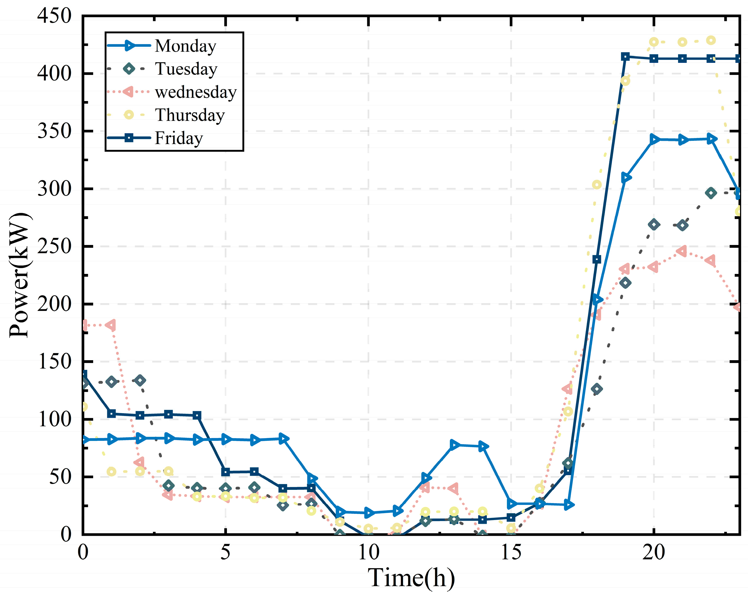
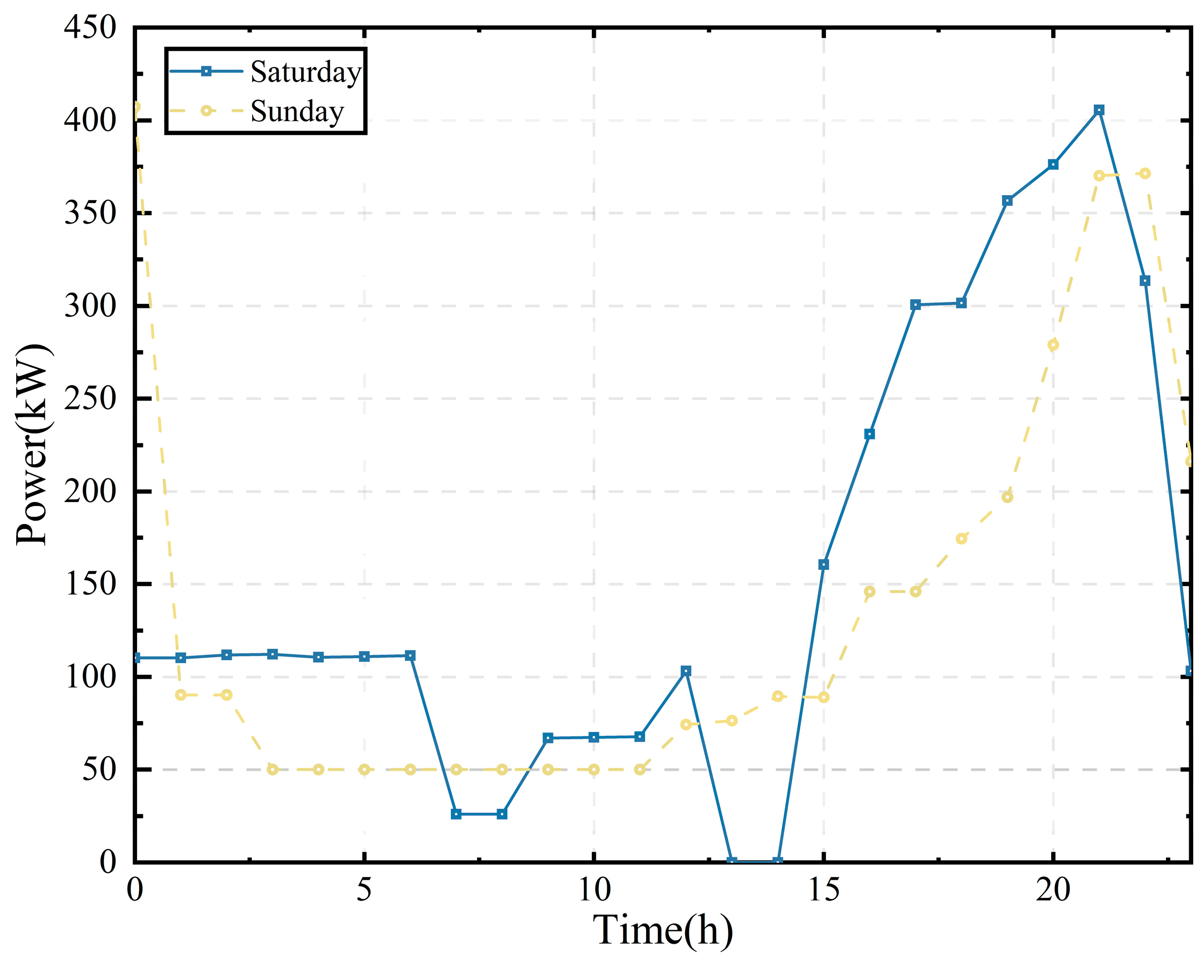
Figure 1. Working day electricity load.
Processes 13 01285 g001
Figure 2. Rest day electricity load.
Processes 13 01285 g002
Figure 3. Flow diagram of SA-BAS algorithm.
Processes 13 01285 g003
Figure 4. Schematic flow diagram of Multi-target Tenox algorithm.
Processes 13 01285 g004
Figure 5. Iterative performance testing of three models.
Processes 13 01285 g005
Figure 6. Three-dimensional space solution set test of three kinds of models.
Processes 13 01285 g006
Figure 7. Flowchart of the two-layer coordination control algorithm.
Processes 13 01285 g007
Figure 8. Improved IEEE33 node model.
Processes 13 01285 g008
Figure 9. The output of the four scenes.
Processes 13 01285 g009
Table 1. The car within a week disorderly charging load (KW.h).
TimeMondayTuesdayWednesdayThursdayFridaySaturdaySunday
Charging load2876219634152757217938643026
Table 2. Peak-to-valley difference rate before and after optimization (%).
TimeEV Load (kw.h)Disorderly ChargingOrderly ChargingDischarge
Monday287645.2335.7830.37
Tuesday219644.2737.4630.2
Wednesday341546.0836.4232.15
Thursday275745.8737.9428.76
Friday217943.5836.9929.68
Saturday386445.9736.2131.64
Sunday302644.4636.1230.16
Table 3. Standard deviation of the equivalent load curve before and after optimization.
TimeDisorderly ChargingOrderly ChargingDischarge
Monday555.84366.84272.50
Tuesday542.44393.32269.07
Wednesday594.34421.39284.78
Thursday533.22404.1258.89
Friday583.17376.45274.23
Saturday570.47379.43279.87
Sunday553.54386269.84
Table 4. Charge and discharge optimization before and after costs (CNY).
TimeDisorderly ChargingOrderly ChargingDischarge
Monday3715.931040.54−458.75
Tuesday2646.44901.26−1053.82
Wednesday4050.091402.8−112.28
Thursday2633.89901.81−1732.5
Friday4013.121680.3−618.68
Saturday4009.751478.86−616.16
Sunday4719.751442−528.57
Table 5. Convergence performance test of three models.
Number of ExperimentsMTTABPSOBFOA
MeanStandardMeanStandardMeanStandard
10.000005420.000003490.000061580.000015630.000614860.00012483
20.000006280.000006700.000054500.000099520.000914820.00001617
30.000001550.000006830.000003630.000029950.000036480.00051666
40.000009520.000009220.000095220.000060420.000318460.00064784
50.000006280.000003850.000039530.000063110.000165420.00016476
Average0.000005820.000006030.000050880.000053710.000415230.00029405
Table 6. Scheduling layer cost in four scenarios (CNY).
ScenarioESSFlexible LoadElectric VehicleGasElectricity PurchasesTotal Cost
S1−602.3681265.4161201.22297.620,437.7524,599.6
S201480.922086.8304021,250.6327,858.35
S3−506.57901272.43347222,302.6326,540.48
S4−602.3681244.460248022,906.3526,028.45
Table 7. Network parameters and EV user costs.
ScenarioNetwork Loss (kW-h)EV User Costs
(CNY)
System Control Costs
(CNY)
Load Curve Standard DeviationTotal Voltage Deviation (%)
S11374.6−1142.825,083.945612.372413.27
S23441.3−1138.125,763.831743.258625.85
Table 8. Cost in both scenarios (CNY).
ScenarioESSFlexible LoadElectric VehicleGasElectricity PurchasesTotal Cost
S1−602.3681265.4161201.22297.620,922.09725,083.945
S2−602.3681265.4161201.22297.621,601.98325,763.831
Disclaimer/Publisher’s Note: The statements, opinions and data contained in all publications are solely those of the individual author(s) and contributor(s) and not of MDPI and/or the editor(s). MDPI and/or the editor(s) disclaim responsibility for any injury to people or property resulting from any ideas, methods, instructions or products referred to in the content.

