Abstract
Delays are known to complicate closed-loop stability analysis and controller design. In the present work, the problem of the stabilization and control of a particular class of linear systems with several real/complex conjugate stable poles and one unstable pole with delay in the direct path is considered. In this work, a methodology is proposed to design a hybrid predictor that consists of continuous and discrete signals to address systems with delay. The proposed hybrid predictor provides a continuous estimation of variables of interest, which is an important consideration, in contrast to the control strategies based on a discrete domain approach. The key point of this proposal is to guarantee the existence of the hybrid predictor, without any restriction on the delay size, when the delay is not divisible by an integer for an appropriate implementation of the sampling period, as in the traditional discrete approach. Furthermore, the proposed methodology is not restricted by the order of the plant, its instability or the size of the delay. The effectiveness of the results is illustrated by numerical simulations performed on academic examples.
1. Introduction
In the process industry and communications, the need to transport material and information, respectively, is very common. These systems are characterised by having a delay term in the dynamics of the process. This phenomenon is called time delay or dead time, and it induces a late reaction in the output response. In the case of chemical processes, this phenomenon is present in systems such as chemical reactors, heating boilers, liquid level systems with a constant output flow, storage tanks, etc. [1,2,3,4,5]. On the other hand, in the case of communication systems, the delay phenomenon is present in the remote control of a mobile robot [6] and aerospace control [7,8]. If the mathematical model of a system with delay is analysed in the Laplace domain, it is observed that if the delay is small enough compared to the dominant time constant of the system, it can be depicted when designing a controller. In the opposite case, if the delay term is considerable compared with the dominant time constant of the system, when closing the control loop, an infinite number of poles are present; this makes it difficult to perform stability analysis and to design controllers, even in the case of reduced-order systems with delay. Thus, the closed-loop output response presents undesirable effects, such as oscillations and even instability. The Smith predictor (SP) [9] is one of the first efficiently designed control strategies for stable systems with delay. This scheme manages to predict the output signal before it is delayed, in order to use it in the control law as if the delay does not exist. In the literature, there are works focused on addressing particular cases of systems with delay due to their complexity, for example, stable systems [9], unstable systems [7,10,11,12,13,14,15,16], systems with real and/or complex poles [17], integrator plus time delay systems [18,19,20,21], first-order plus time delay systems [15,16,18], second-order plus time delay systems [14,15,16], and higher-order systems [15,17,18,20,22,23,24]. Some approaches to address systems with delay include modifications of the Smith predictor (SP) [7], PI/PD/PID controllers [5,11,14,15,16,25], two-degrees-of-freedom control [3,18,26], the observer-based approach [11,13,20,24,27], predictive controllers [28], internal model controllers [29], fractional-order controllers [30], etc. In the specific case of unstable delayed processes, these systems are characterised by limitations in terms of stability and performance when closing the control loop. In this way, in [31], a simple modification of the Smith predictor was proposed, dealing with systems with one unstable pole but restricted to relatively small delays. Another approach used to address delayed systems is the digital computer control approach. In the discrete approach presented in [13,18,32], as well as many traditional discrete strategies for delayed systems, the sampling period T must be selected such that , where is the size of the delay and n is any integer. Note that may be a restriction when applying the physical implementation of the controller if the sampling period T is a periodic (pure or mixed) or aperiodic rational number, due to the fact that it is desirable to obtain an exact rational number with one or two digits for the simplicity of the physical implementation of the sample period T; rounding may induce unnecessary uncertainty in the control loop. Proposing strategies for systems with delay is still an open topic of research, with the goal being to find a solution to more general cases, due to the complexity of modelling these systems with delay. In this work, the case of high-order systems with any magnitude of delay is addressed, where the delay is considered to be in the direct path, either at the input or at the output. The proposed methodology consists of designing a controller based on a hybrid predictor that guarantees the stability of the system with delay. This methodology uses the discrete model for the design of a control scheme, proposing an alternative to the aforementioned restriction on the sampling period, . Thus, with the proposed methodology, the total delay is distributed as . Therefore, the designer ensures that in the part to be discretised, the selected sampling period is not a periodic/aperiodic number. In this way, the restriction imposed by the sampling period can be tackled. The proposal uses a result previously published in [33], where a predictor is designed from the discrete model and the injection of discrete signals. Some strategies extend the ideas of the compensator to unstable delayed systems [3,9,24,34,35,36]. Some of these papers [32,36,37,38,39,40,41] affirm that there is no way to avoid a discrete-domain analysis to obtain an estimation of the variables. In the present paper, the estimated signals obtained from the proposed predictor are continuous; however, the predictor contains a discrete injection stage. In this way, we introduce a hybrid strategy. This work presents a methodology that includes the design of the hybrid (discrete-based) predictor and a continuous controller , with the objective of stabilising high-order delayed linear systems with one unstable pole and several real/complex conjugate stable poles and with a delay of any magnitude, without imposing the restriction .
The work is organised as follows. Section 2 presents the problem statement and the preliminary results, where the essence of the proposed hybrid predictor is described based on an illustrative example. Subsequently, in Section 3, the main results for a particular class of high-order linear systems are presented and the main contribution of this work is shown, that is, the proposal of a control scheme based on the hybrid prediction scheme, which does not require the restriction . In Section 4, some numerical examples with a large delay are presented to illustrate the effectiveness of the proposed strategy. Finally, some conclusions are presented in Section 5.
2. Preliminary Results
This section presents a digital control methodology that gives an introduction to the concepts of the strategy proposed in this work. In order to simplify this explanation, the second order is used. Consider a continuous-time linear system given by the transfer function :
where . A state-space representation for the system (1) can be written as:
with , and
Then, consider a zero-order hold and a sampling period T; the discrete representation of the transfer function (1) is given as follows:
where , , , and . Also, consider the following state-space representation for the discrete system (4):
where , , and .
In what follows, an analysis of the previous representations is presented to explain an important problem when it comes to using them for a state feedback control and injection output strategy.
2.1. Discrete State Feedback
Note that if a digital control methodology based on state feedback, as shown in Figure 1 for the system (1), is proposed, the state-space representation (5) and (6) is not useful for calculating the control parameters and . This is because the relationship between the input and the state in the continuous original system is lost, due to the chosen discrete state-space representation (5) and (6). This means that the information of state of the continuous system does not coincide with the obtained information of state from the discrete representation (5) and (6) in the sampling instants. Thus, in order to obtain a discrete state representation that does not lose the input–state relationship, the following expressions, presented in [42], should be used:
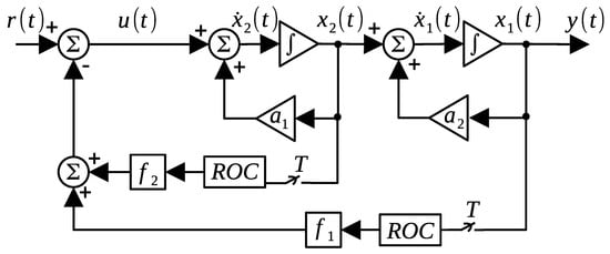
Figure 1.
Static state feedback.
Finally, to find the values of the gains and , the closed-loop characteristic equation, , and a desired closed-loop characteristic equation, , are equated. , I is an identity matrix of size , and and are the desired locations (within the unit circle to achieve stability) of the closed-loop poles of the system shown in Figure 1.
Next, the MATLAB (R2024a) commands to obtain discrete state feedback are presented. First, the system in the continuous-time state-space given by (2) and (3), with , is defined. Then, considering a sampling period T, it is possible to obtain the desired discrete version, shown in (7)–(10), with the command . Finally, with the command , the gain value can be found, where and are obtained from the representation.
2.2. Discrete Output Injection
Consider the system (1) and the discrete output injection shown in Figure 2. Note that there is also the possibility of choosing a discrete representation for (1), in such a way that the state-output relationship is lost in the injection scheme. Thus, with the objective of obtaining a state-space realization that recognises the adequate mapping from the state-space variables to the output, it is not complicated to make a dualization of the relations in (7)–(10), as shown below:
where denotes the transpose of ∗.

Figure 2.
Output injection.
Finally, the matrices in (11)–(14) are used to calculate the gains of the vector associated with discrete injection. This can be done by equating the closed-loop characteristic equation, , and the desired closed-loop characteristic equation, , where and are the desired locations (within the unit circle) of the closed-loop poles of the injection scheme, shown in Figure 2.
The above procedure can be also calculated by using MATLAB commands. First, the continuous system is defined with the command , and the discrete version is obtained with the command , where T is the sampling period. Thus, contains the auxiliary matrices required to perform discrete injection. Finally, these matrices are used to calculate the gains of the vector G associated with the discrete injection; this can be done by using the command , with and
Note that the state-space representation given by (11)–(14) is not required when a traditional digital based observer/predictor is designed. However, state-space representation (11)–(14) must be considered when a continuous estimated variables are required as it is the case of the proposed predictor scheme in this work.
2.3. Controller Design
The following result establishes the stability condition for implementing a PID controller for an unstable system with time delay. This result is presented in [17] for a general system with possible complex conjugate stable poles. In this paper, it is used the simple version of the result for the particular case of only real poles as presented in [22].
Lemma 1
([17,22]). Let us consider the high-order unstable system defined by
and a PID controller defined in [43] as follows:
where is the derivative time, the integral time, and K the proportional gain. Then there exists such that the closed-loop system (with ) is stable if and only if
The stabilising parameters for the control , associated with Lemma 1, can be obtained as follows. First, the parameter is chosen from
After this, to find the set of stabilising gains K, it is necessary to obtain the first two positive frequencies (denoted as and ) of the following expression, with
Then, the parameter can be obtained by sweeping such that (18) has two positive solutions close to the case when . Finally, the set of stabilising gains K is given by
with
and .
2.4. Problem Statement
The type of system addressed in this work is given by
where , , with . For the sake of simplicity, the control proposal is developed for the case when contains real poles; then, the proposed control strategy is extended to the case of containing pairs of complex conjugate stable poles. The main idea of this paper is to propose a control scheme based on the feedback of an estimated (predicted) continuous signal generated by a continuous predictor tuned by an injected discrete error signal.
3. Main Results
To design a prediction strategy, consider a division of the delay in the transfer function (20), defined by
where . Note that this consideration is only taken up for proposal design. Now, consider a state-space representation of the transfer function (21) free of delays and , i.e., considering , given by
where
Now, consider and the sampling period (where ) and a zero-order hold . A discrete state-space representation of the system, (22) and (23), and the formulation (11)–(14), can be given by
with , , and . Note that the addition of the delay in (24) and (25) results in n poles at the origin, that is, . A representation in discrete state-space for with , can be written as
where
with , , and .
In this way, using the discrete representations in state-space given by (24)–(27) of the delay-free system and the delay , respectively, it is possible to write a whole representation in state-space of the transfer function (21):
where
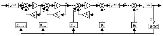
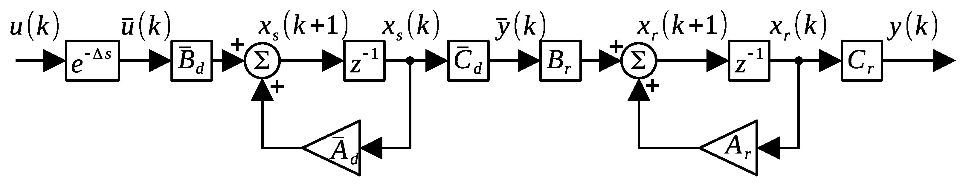
Therefore, Figure 3 shows a representation for the system given by (21) without discretization . The size of the matrices obtained, , and , increases in relation to the number of delay partitions n. From the hybrid representation (28) and the discrete output injection strategy, presented in Section 2.2, it is possible to design an estimation strategy (hybrid predictor) for the system given by (21).
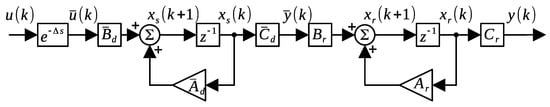
Figure 3.
State-space discrete representation of (21).
Next, a result related to an output injection for the system (21) is presented.
Lemma 2.
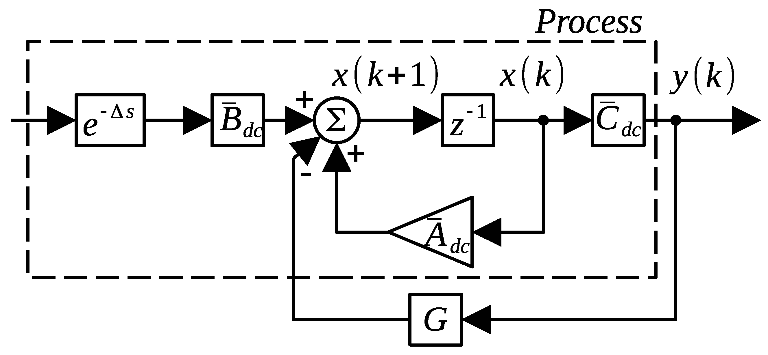
Consider the system given by (21) and the output injection diagram shown in Figure 4. Then, there is a gains vector such that the injection scheme shown in Figure 4 is stable.
Figure 4.
Proposed output injection scheme.
Proof.

A discrete state-space representation of the output injection scheme shown in Figure 4, with a sampling period , is given by
with . The representation (30) and (31) is presented in Figure 5 in a block diagram. This can be verified using the hybrid representation of the system given by (21), which is given by (28).
Figure 5.
The discrete equivalent of the injection diagram shown in Figure 4.
Note that the representation (30) and (31) is equivalent to the scheme in Figure 4 at sampling instants T. It is important to observe that the injection scheme shown in Figure 4 is hybrid (continuous-discrete). However, the equivalence in the sampling times is valid due to the sampler and zero-order hold, which are present in the injection diagram shown in Figure 4; the proposed partitions of the delay are also shown in this figure.
Thus, by considering that the discrete state-space representation (, ,) is a minimal realization because it comes from a transfer function, it can be concluded that the system is observable and therefore there is a vector such that has its roots inside the unit circle. These facts allow us to prove the statement of the lemma. □
One way to calculate the gains vector involved in Lemma 2 can be realised by developing the expression and equating the left side of this expression with the left side of a desired polynomial , which contains the desired location of the closed-loop poles. It should be noted that the proposed desired polynomial must be of the same order as , that is, . These desired locations must be proposed within the unit circle to ensure that the closed-loop system is stable. Another alternative for calculating the stabilising vector G is to use the following MATLAB commands: or . For example, , where , , are the desired locations, within the unit circle of the closed-loop poles.
By using Lemma 2, it is possible to design an estimation strategy. In this case, a hybrid predictor for the system given by (21).
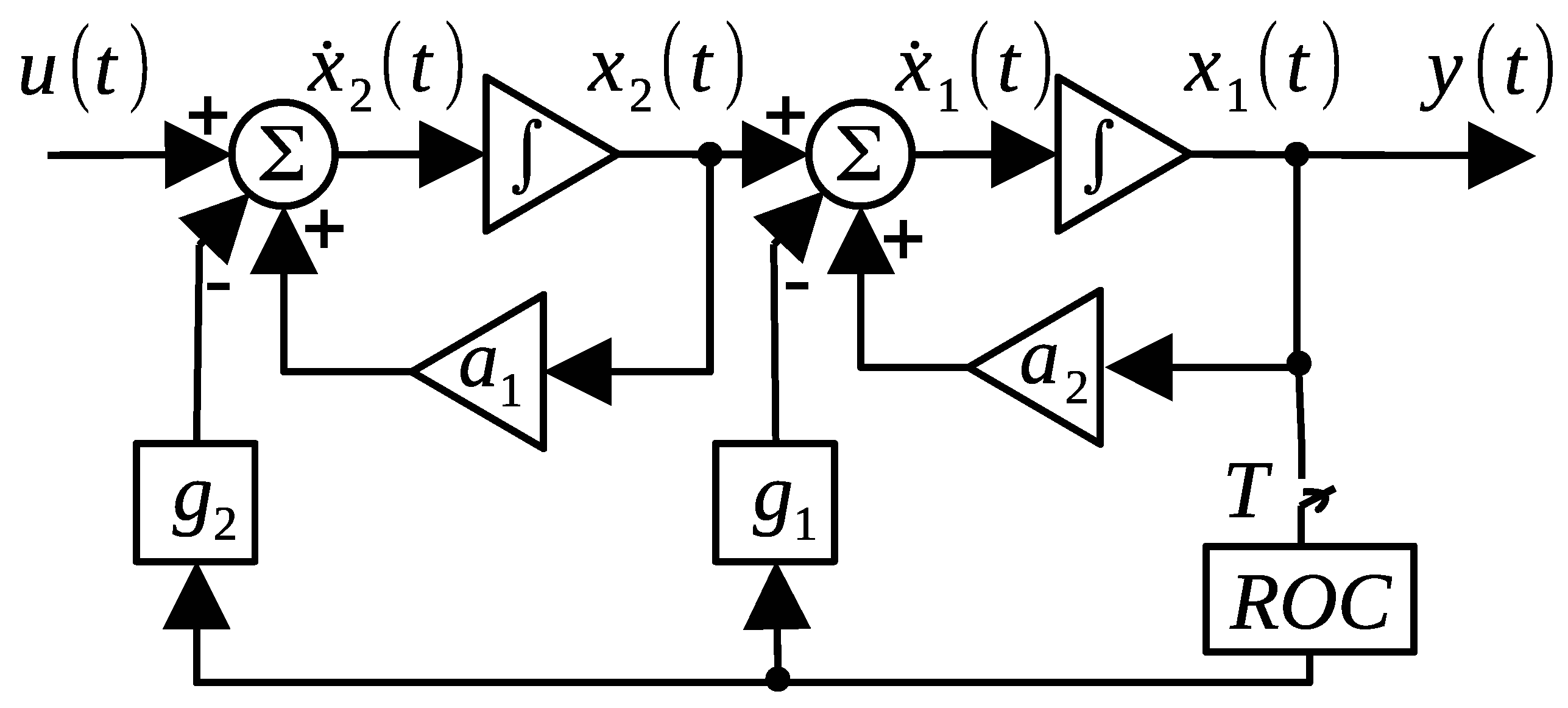
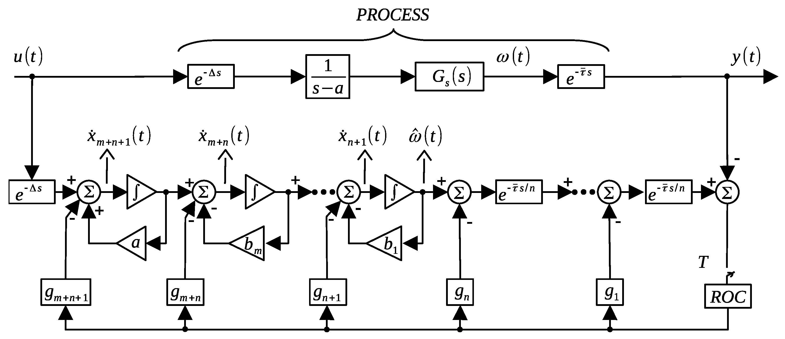
Below, a result related to the adequate estimation of the variables in the proposed prediction scheme shown in Figure 6 is presented.

Figure 6.
Hybrid predictor.
Lemma 3.
Proof.
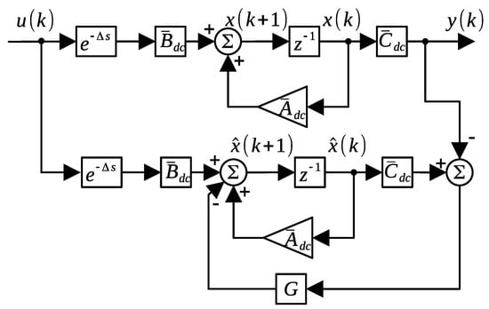
The proof consists of considering the hybrid representation in state space for the system (21), given by (28), and the hybrid predictor shown in Figure 6, represented as follows:
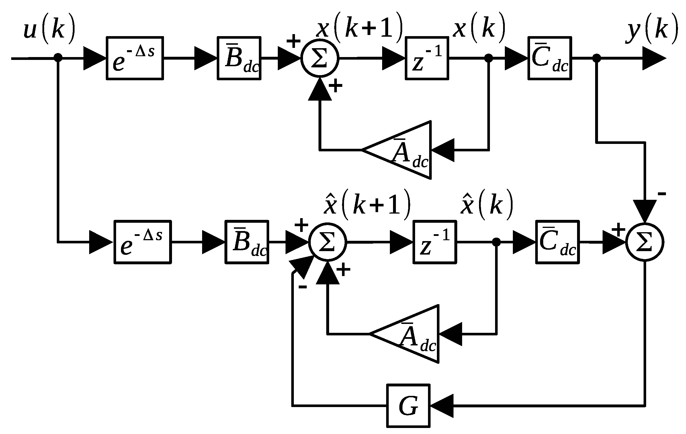
Thediscrete diagram shown in Figure 7 is equivalent to the scheme of Figure 6 at the sampling instants T. Although it is true that the proposed hybrid predictor scheme shown in Figure 6 contains some analogue elements, such as the integrating blocks and the delay blocks, the equivalence in the sampling times between both presented schemes is due to the presence of the sampler and zero-order hold, which can be found in the diagram shown in Figure 6, along with the proposed partitions of the delay .
Figure 7.
Discrete equivalent of the proposed hybrid predictor.
Subsequently, in the scheme of Figure 7, the estimation errors are defined as , where , and the dynamic errors are calculated, resulting in
where and with .
Note that the dynamics of the convergence error expressed by the Equation (33) have the same form as the dynamics of the output injection scheme presented in Lemma 2; this can be verified by comparing the Equation (33) with the state-space representation of the output injection scheme in closed-loop form, given by (30) and (31). This allows us to conclude that in the scheme of Figure 7 and therefore in the scheme of Figure 6, because at sampling instants T. Note that even though the injection scheme given by the Equations (30) and (31) has an input and the convergence expression given by (33) has no external input, the stability conditions are the same because external inputs do not affect the stability of a system.
It can be verified that the errors tend to zero as k tends to infinity, or ) if, and only if, has its roots inside the unit circle under the assumption that the discrete state-space representation , , and is observable. □
Lemma 3 ensures the adequate estimation of the variables for the plant given by (21). Additionally, the parameter G of the proposed predictor can be calculated as the parameter G involved in Lemma 2; this procedure is presented after the proof of Lemma 2. Now, by using the estimated plant signal variable, , it is possible to design the control stage. The following result addresses this issue.
In what follows, the stability conditions based on the proposed hybrid predictor for the closed-loop system are stated.
Theorem 1.
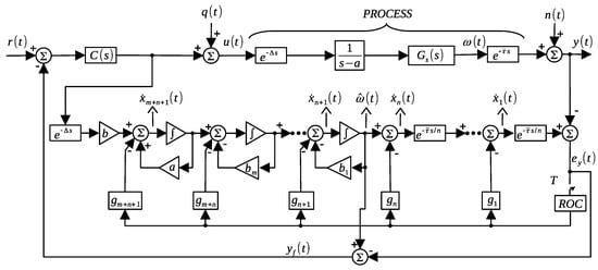
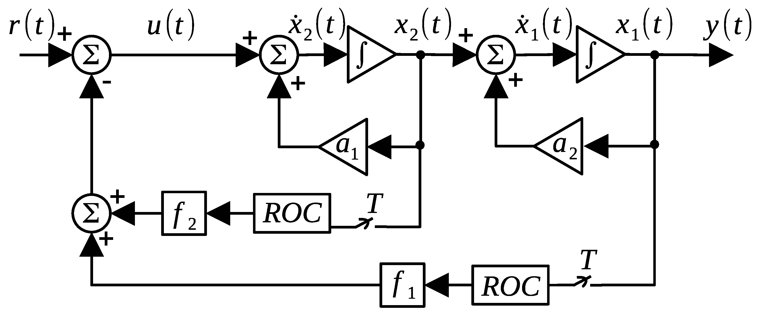
Consider the system (21), a PID control and the hybrid predictor shown in Figure 8. Then, there exist gains and a control , such that the system in the closed loop of Figure 8 is stable if and only if
Figure 8.
Proposed control strategy based on a hybrid predictor.
Proof.
Considering Lemma 3, it is possible to obtain a vector G such that an adequate estimate is achieved for . Then, considering that the separation principle is a property of linear systems, it is possible to design the control stage using the estimated signals; in this case, a PID control to stabilise the system is proposed. By using Lemma 1, there exists a control stabilising such that the associated closed-loop system is stable if, and only if, □
Theorem 1 states that the stability condition used to apply the proposed control strategy based on a hybrid predictor of Figure 8 is derived from controlling the unstable system using a controller .
It is important to note that once an adequate estimation is achieved, it is possible to propose any control strategy for the high-order unstable system (15). The scheme shown in Figure 8 is capable of following a step-type reference and guarantees the rejection of step-type disturbances when a controller with integral action is used; these characteristics are achieved due to the proposed feedback based on the original . The parameters of the controller can be calculated using results related to Lemma 1.
The proposal of the presented scheme is essentially the need to eliminate the restriction when the predictor design is carried out, since sometimes the period of sampling T from such a condition may be non-functional for design and implementation, especially when the sampling period is not an exact rational number, as this is not easy to implement physically.
Taking into account the above, in this work, it is proposed to divide the delay (in the design of the strategy) in such a way that the delay is a decimal number with a single significant cipher and contains the other part of the original delay (). It is proposed that the delay be small compared to the other fraction of the delay , since if the delay is small (as suggested in this work), there are more possibilities to achieve a better output performance of the controlled system, due to the fact that in an unstable linear first-order system with delay, if the delay increases, the interval of stabilising gains of a proportional control decreases, resulting in a restriction on the controller design.
Hybrid Predictor for Delayed Systems with Complex Conjugate Stable Poles
Consider the class of systems of (20), with
which is a partition of the delay , as defined in (21), with (34). Thus, the proposed hybrid observer shown in Figure 8 can be easily performed for the class of systems in (20)–(34) by only considering a state-space representation of (34) in all the developments presented above. In what follows, a similar result of Theorem 1 is presented for the class of systems (20)–(34).
Corollary 1.
Proof.
The proof is similar to the proof of Theorem 1; it involves considering the control stability result of a system with one unstable pole, n pairs of complex conjugate stable poles and delay controlled by control [17]. □
Note that Corollary 1 considering a controller provides the tracking of references, as well as the disturbance rejection of step signals.
4. Simulation Results
Now, in order to evaluate the proposal, some numerical simulations are presented; these simulations were carried out using Simulink, which is based on MATLAB software.
4.1. Example 1
Consider a third-order unstable process, from [15,23], where the delay size has been modified, given by
To ensure the stability of the system (35), it is proposed to partition the delay , as proposed in (21); in this example, and . Considering the expressions (22) and (23), the representation in state space for the system (35) free of delays and can be written as
Now, considering that , it is proposed that to obtain the sampling period; thus,
In this case, note that the sample period obtained in (38) is a convenient sample period for the hybrid predictor design, since it is an exact rational number. Note that if the partition , and would have been considered, and the sampling period would be , which would be difficult to implement physically in the control diagram proposed in Figure 8.
A discrete state-space representation of (36) and (37), with a sampling period (38), is given by (28), with
Now, with these matrices, the values of G are calculated such that is stable. To do this, it is proposed to locate the poles of the characteristic equation at ; the value of the vector G that satisfies the aforementioned characteristics is described below:
With the vector G given in (42), the convergence between the estimated signal and the original signal is ensured in the scheme of Figure 8 (Lemma 3).
Next, the values of the parameters , and K of the control are obtained with Lemma 1 for the system . By considering from (17) and plugging into (18), and are obtained. Finally, from (19), is chosen. Then, the control from (16) is given by
Finally, to improve the output response, a controller with two degrees of freedom [43], given by , is considered, with
where and should be selected from and . Notice that different values of and respond to load disturbances and measurement noise in the same way. For the simulations, .
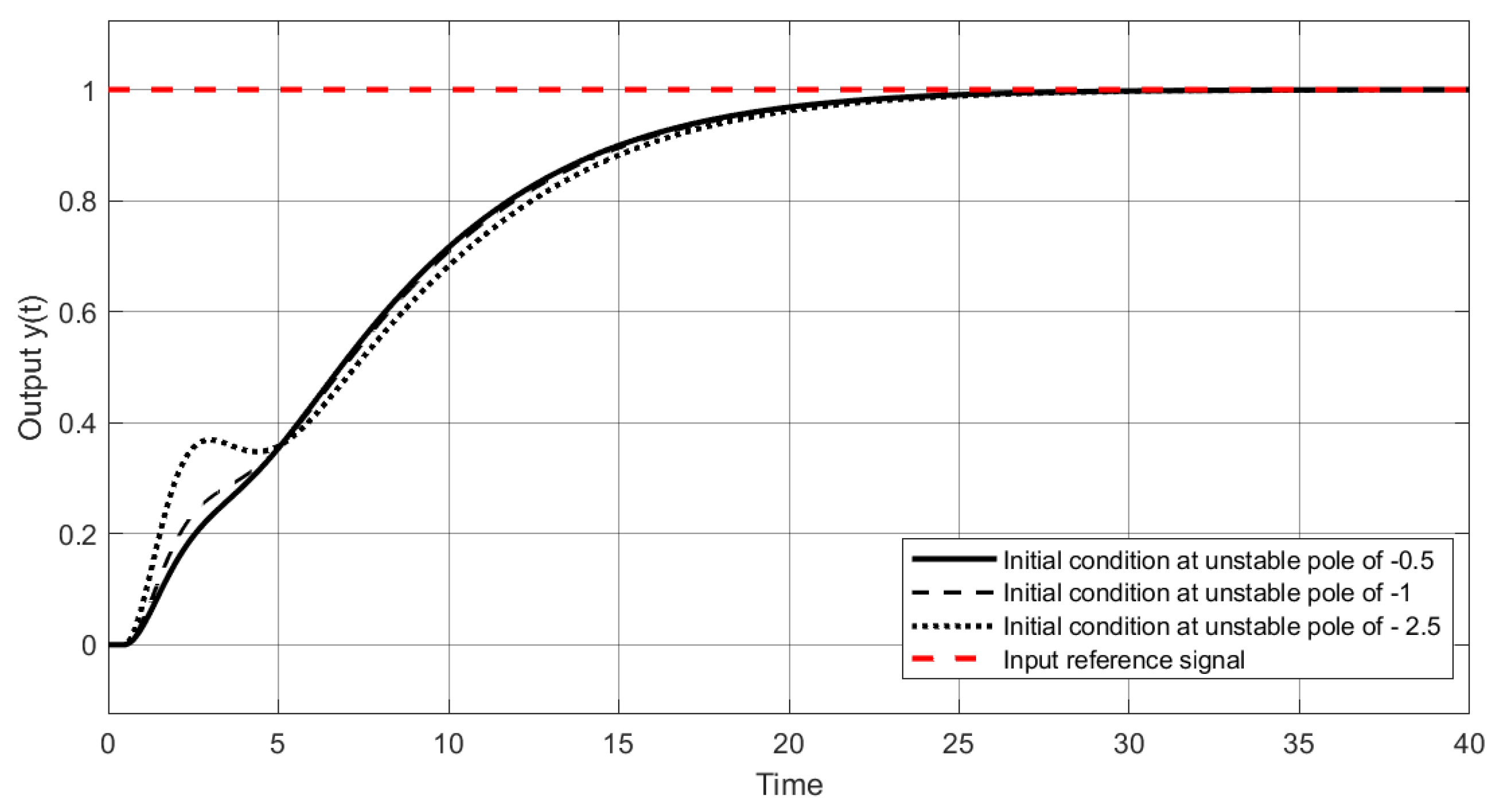
The closed-loop output responses with the proposed hybrid predictor are presented in Figure 9. The output responses are stable considering different initial conditions in the unstable pole of the plant of magnitudes and . Also, for the simulation, a unit step input reference is considered.
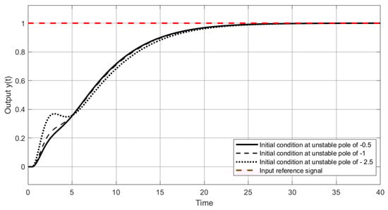
Figure 9.
Output response with different initial conditions for Example 1.
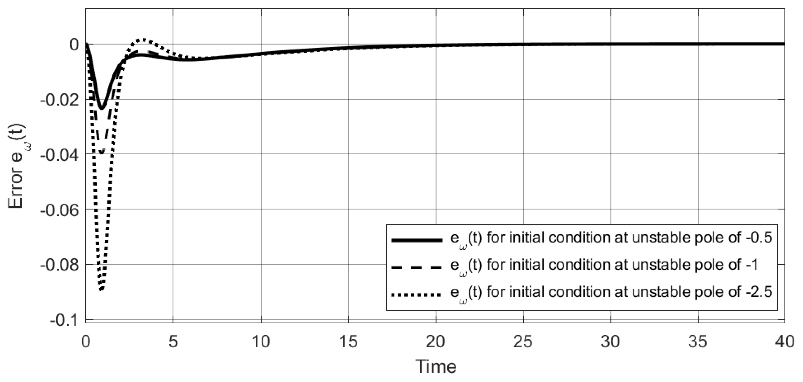
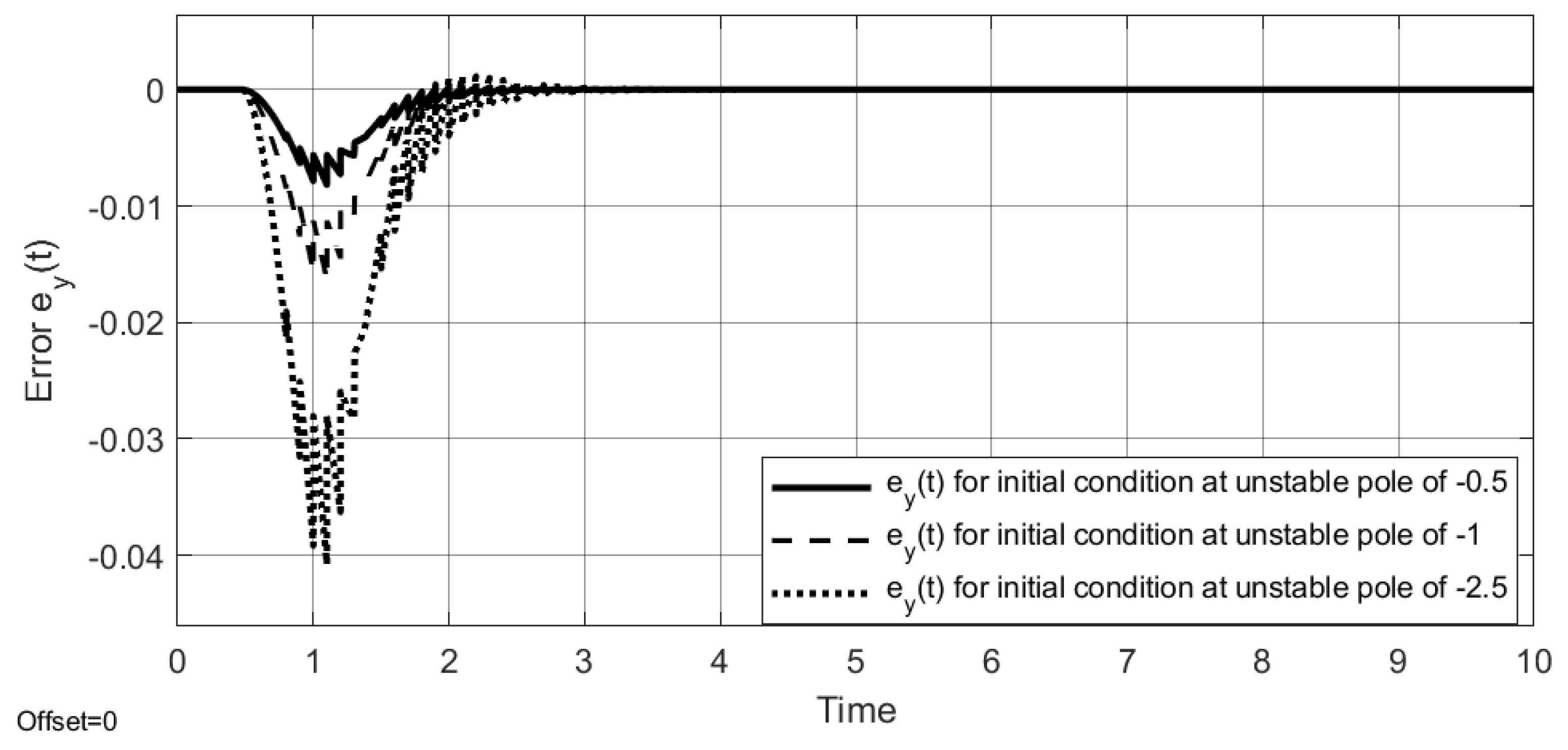
The estimation error signals for different initial conditions are shown in Figure 10; in this example, it is possible to verify that this signal tends to zero in a steady state, and therefore the proposed strategy makes an adequate estimation of the variable of interest. Further, under the same conditions, the system output error signals are presented in Figure 11.
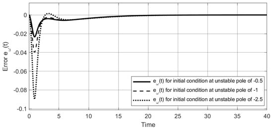
Figure 10.
Output estimation error with different initial conditions for Example 1.

Figure 11.
Output estimation error with different initial conditions for Example 1.
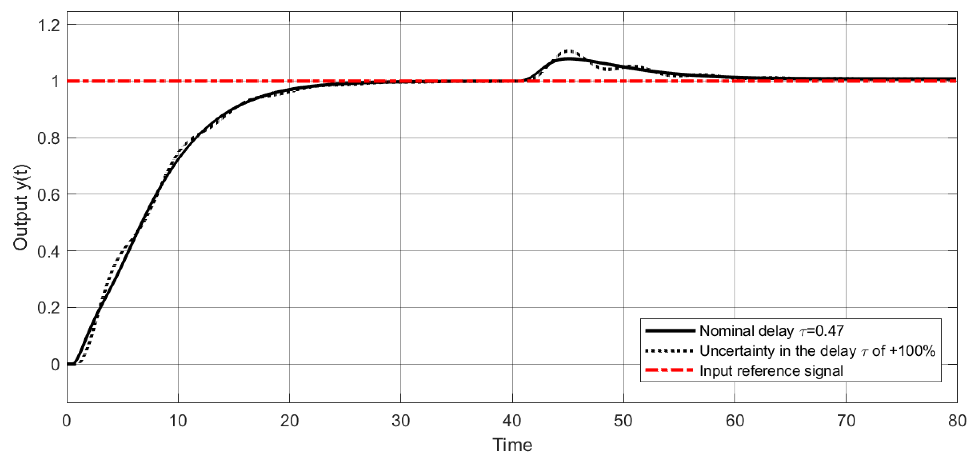
In Figure 12, a solid line shows the output response when the exact knowledge of the model parameters is considered; a dashed line presents the output signal when the time delay is increased by . In the simulation, , a disturbance acting at and an initial condition in the unstable pole of the plant of magnitude are used. Also, it can be seen that the strategy allows disturbance rejection and reference tracking even when the delay-time size is not the nominal value.

Figure 12.
Output response to uncertainty in the delay for Example 1.
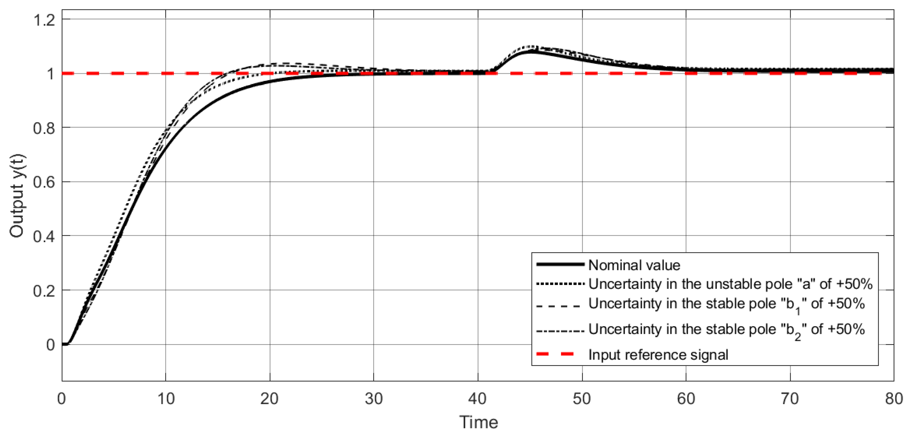
Figure 13 illustrates the system performance in the nominal case with a solid line and the different cases when uncertain parameters are considered. For the simulation, and acting at and an initial condition in the unstable pole of the plant of units are considered. In this example, the proposed control strategy allows the system to deal with model uncertainty; however, the percentages of uncertainties can be variable due to the time-delay magnitude, the order of the system, the gain tuning, etc.
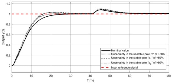
Figure 13.
Output response to uncertainty in the plant for Example 1.
Figure 14 shows the output response for white noise effects at the output measurement. It can be observed that system stability prevails over such effects. Finally, Table 1 presents the evaluation results for different performance indicators: the integral quadratic error criterion (ISE), the integral of quadratic error multiplied by the time (ITSE), the integral absolute error (IAE), and the integral of absolute error multiplied by the time (ITAE). The results presented in Table 1 correspond to measurements performed on control action and the output signal , considering the initial condition of at the unstable pole of the plant.
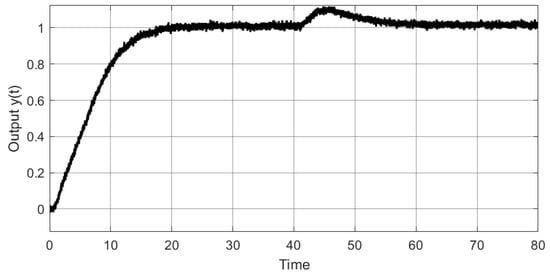
Figure 14.
Output response to noise effects of Example 1.
4.2. Example 2
Consider an unstable high-order time delay process, taken from [44], where the delay size has been modified, given by
First, consider the partitioning of the delay , as proposed in (21), with and . Then, using the expressions (22) and (23), the representation in state space for the system (45), free of delays and , is given by
Let us consider that and that ; thus,
This sampling period will be used in the hybrid predictor design. In order to obtain a discrete state-space representation of the representation in state space (46) and (47), with a sampling period (48), (28) is considered, with
Once these matrices are obtained, it is possible to calculate the values of G such that is stable. The poles of the characteristic equation are located at ; therefore,
Then, with the vector G presented in (52), in the scheme of Figure 8 (Lemma 3), convergence between the estimated signal and the original signal is ensured.
Using Lemma 1, the values of , and for the system are obtained. For the control given by (16), the following is obtained:
Additionally, in order to achieve a better response, the controller with two degrees of freedom [43], defined in (44), is implemented, where for the simulation.
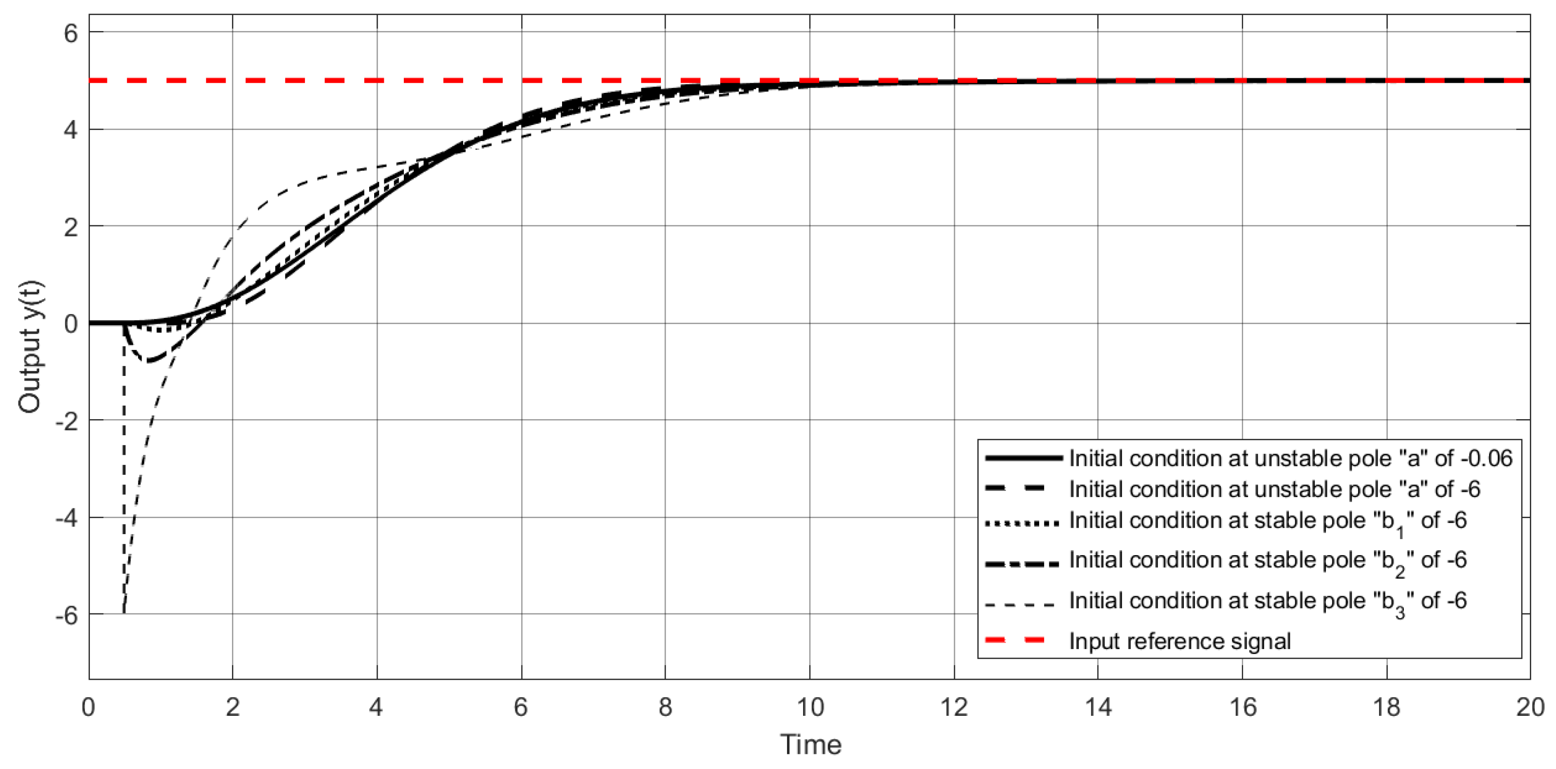
The hybrid predictor produces closed-loop output responses , as seen in Figure 15. These responses are stable considering different initial conditions in different poles, as shown. For the simulation, a step input reference is used.
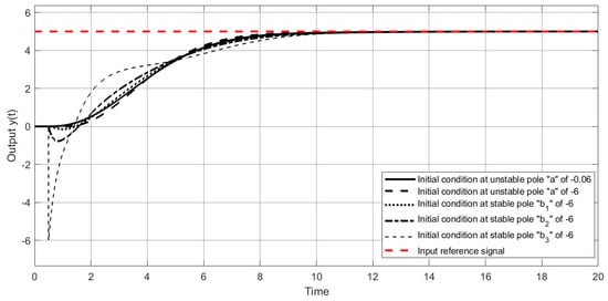
Figure 15.
Output response with different initial conditions in the states for Example 2.
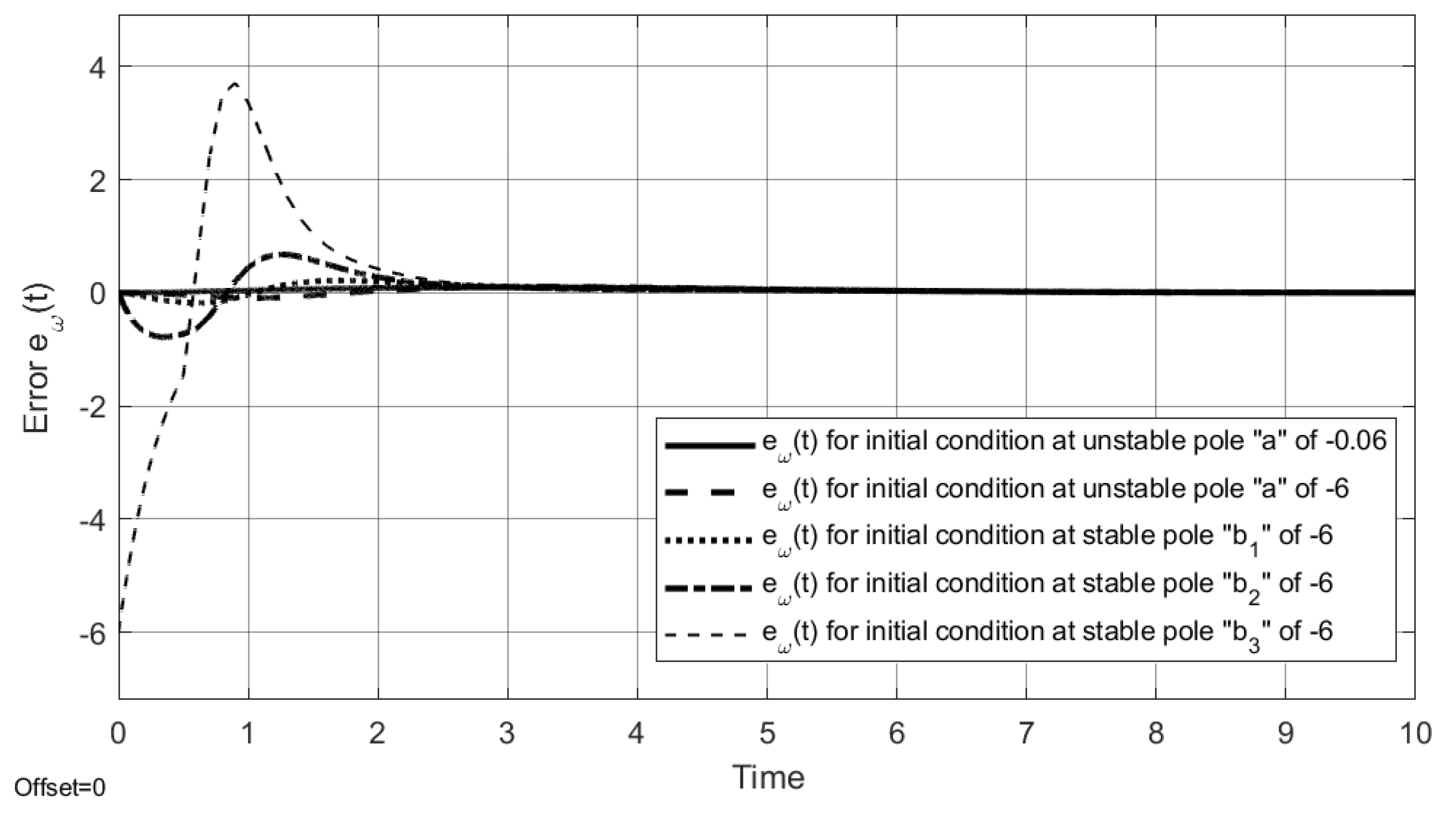
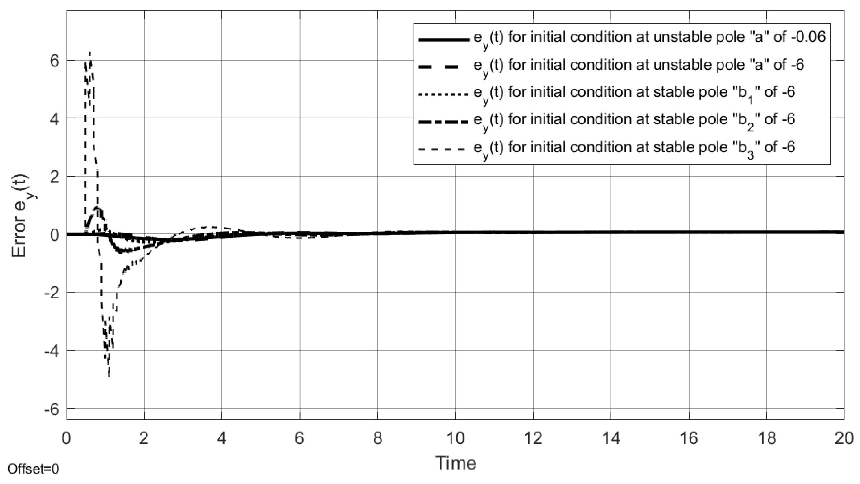
The estimation error signals and the system output error signals are presented in Figure 16 and Figure 17, respectively, for different initial conditions.
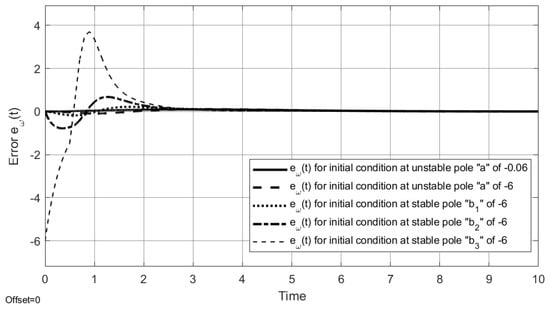
Figure 16.
Output estimation error with different initial conditions for Example 2.
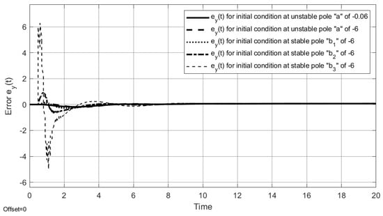
Figure 17.
Output estimation error with different initial conditions for Example 2.
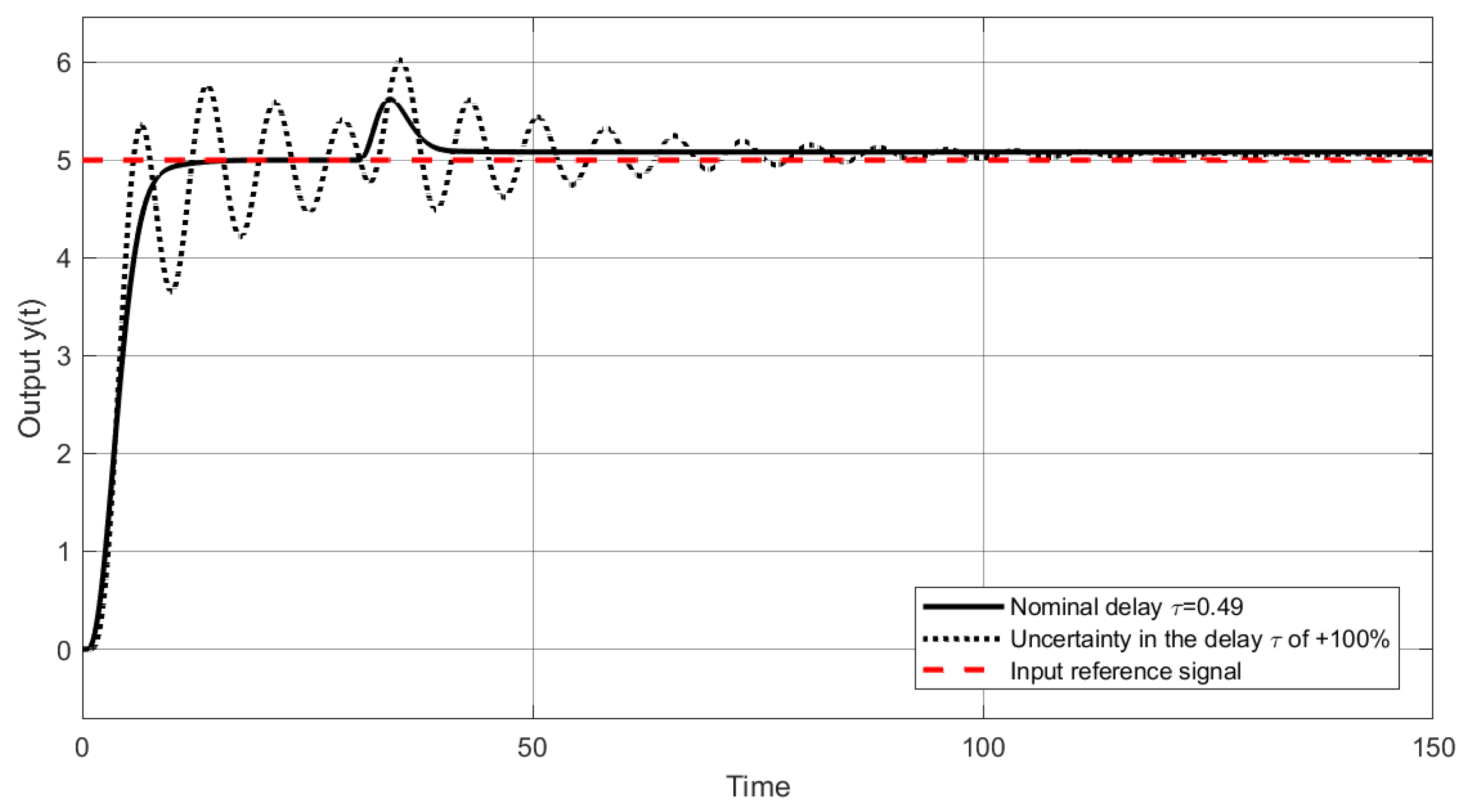
In Figure 18, the output responses are displayed with a solid line in the nominal case, and in the case of , the dashed line represents the time-delay increase. In this case, , a disturbance acts at and there is an initial condition in the unstable pole of the plant of magnitude . The strategy is capable of disturbance rejection and reference tracking, as can be seen.
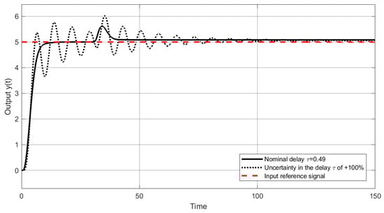
Figure 18.
Output response to uncertainty in the delay for Example 2.
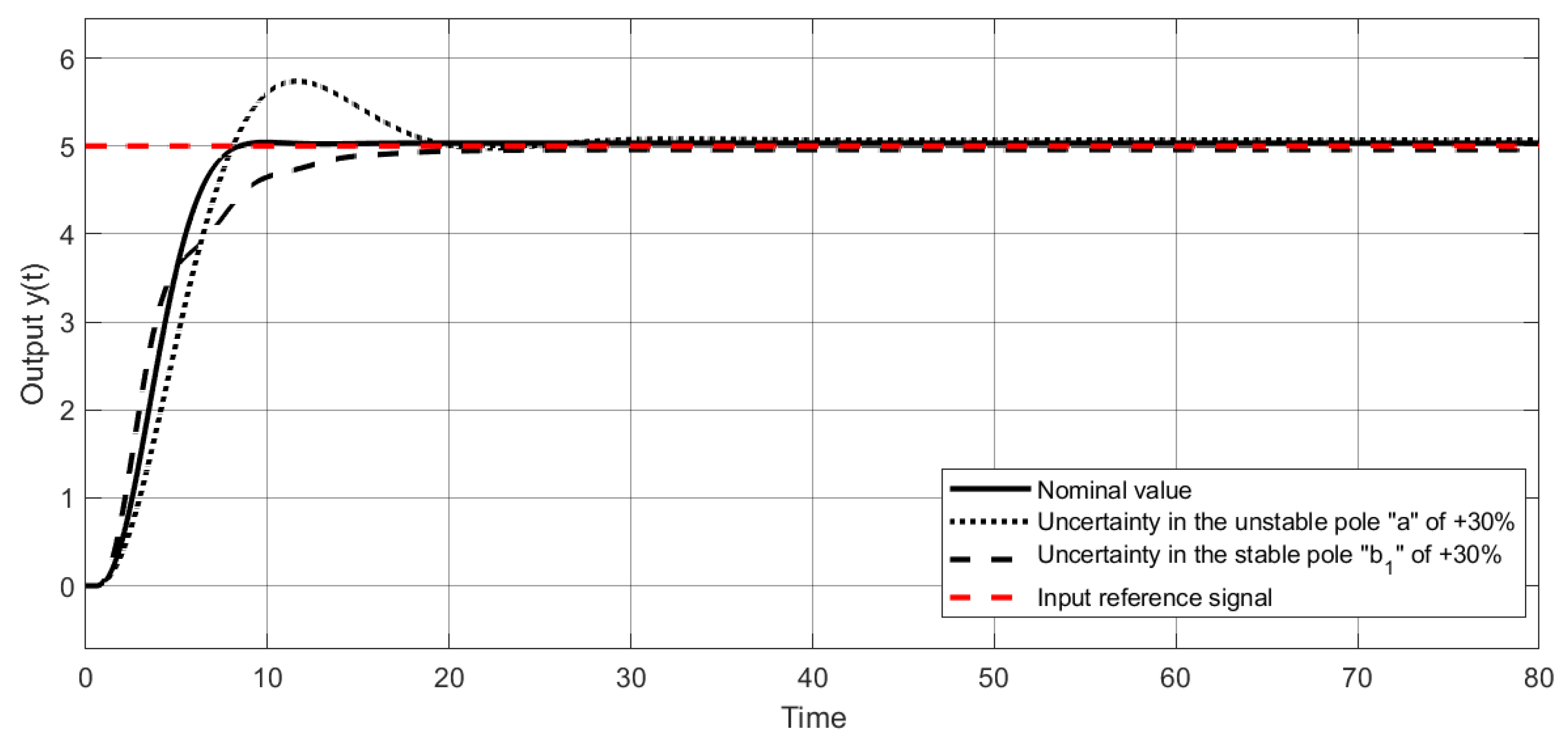
The system performance in the nominal case is shown in Figure 19 with a solid line. Also, in Figure 19, different cases are considered when there is uncertainty in the parameters, with and an initial condition in the unstable pole of the plant of magnitude for the simulation. A quantitative analysis of the closed-loop system behavior was performed, the control signal and the output signal are evaluated by using different performance indicators. The results obtained are shown in Table 1, where initial condition at the unstable pole of the system with a value of −0.06 is considered.

Table 1.
Comparative table of quantitative evaluation of the Examples 1 and 2.
Table 1.
Comparative table of quantitative evaluation of the Examples 1 and 2.
| Example 1 | Example 2 | |||||||
|---|---|---|---|---|---|---|---|---|
| System | ||||||||
| Control Action | ||||||||
| Performance index | ISE | ITSE | IAE | ITAE | ISE | ITSE | IAE | ITAE |
| Hybrid predictor | 128.8 | 3129 | 72.95 | 3153 | 152.2 | 1450 | 24.04 | 237.7 |
| Output | ||||||||
| Performance index | ISE | ITSE | IAE | ITAE | ISE | ITSE | IAE | ITAE |
| Hybrid predictor | 69.41 | 3129 | 72.27 | 3156 | 365.8 | 4588 | 78.65 | 944 |
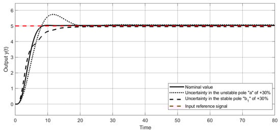
Figure 19.
Output response to uncertainty in the plant for Example 2.
4.3. Example 3
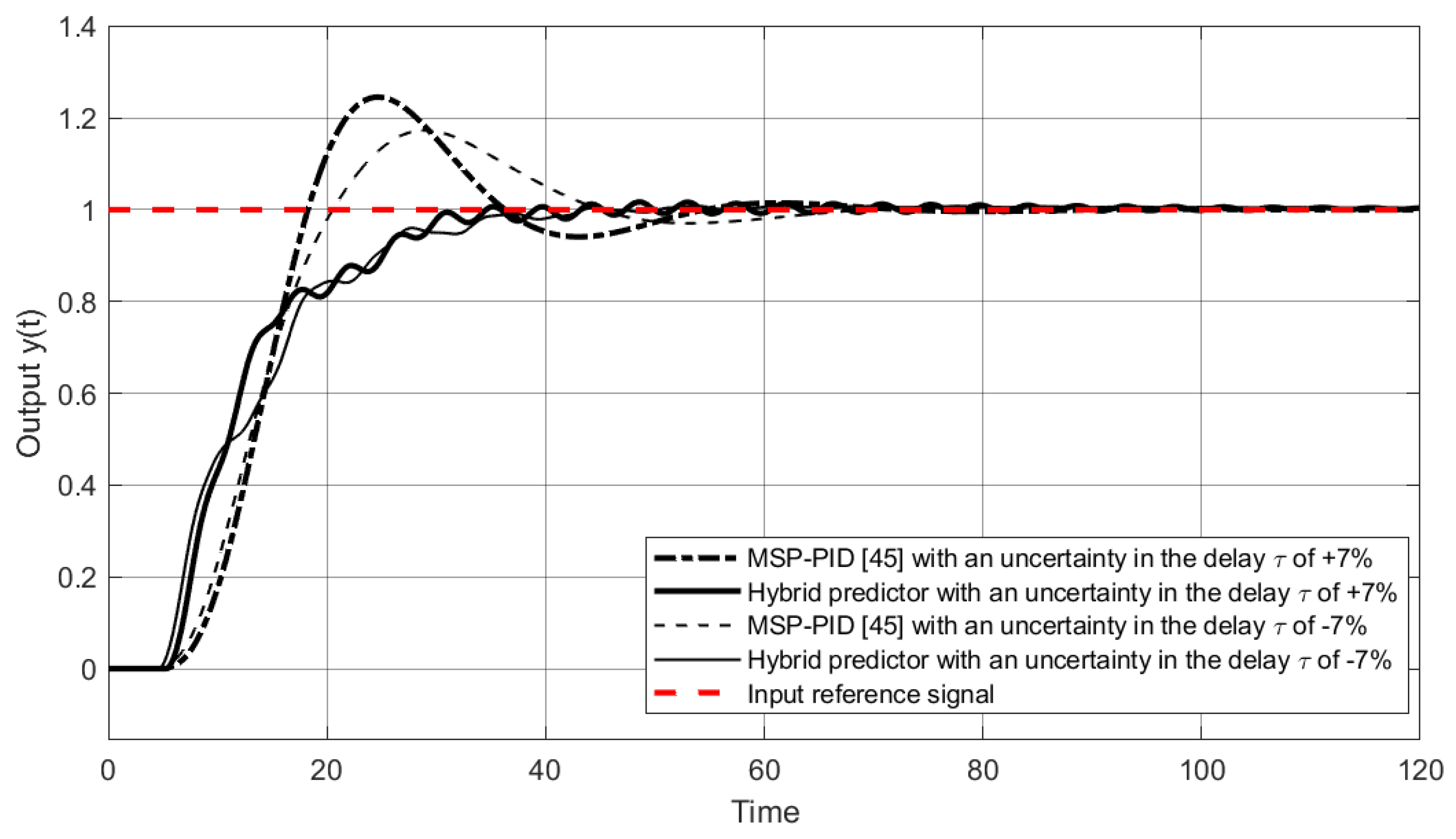
Let us consider the second-order unstable system with time delay previously studied in [45],
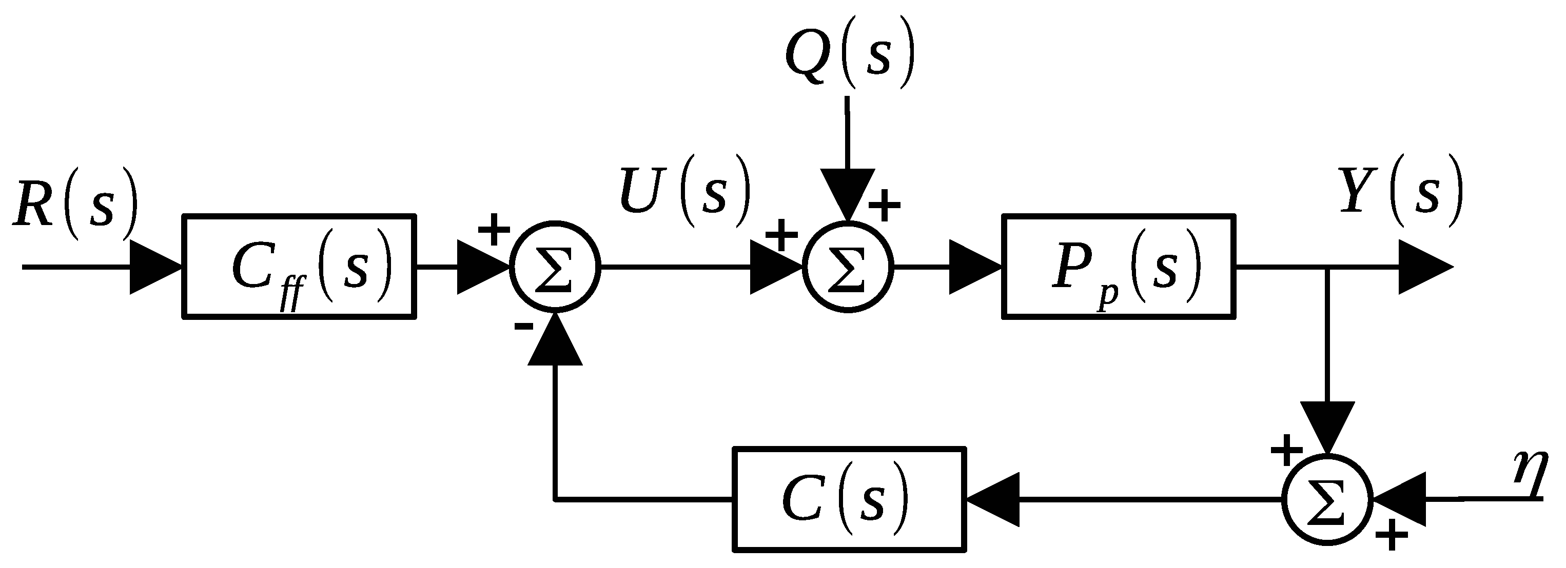
In the scheme proposed in [45] (see Figure 20), a modification to the Smith predictor (MSP), implemented under a PID structure with filter (MSP-PID), is presented. In the scheme proposed in [45], specifically in the MSP-PID configuration, the following controllers are used.
for the output feedback,
as a pre-filter and for the set-point tracking,
where , , , , , , , , and with . These parameters are the result of an optimization process where the delayed plant model is used.
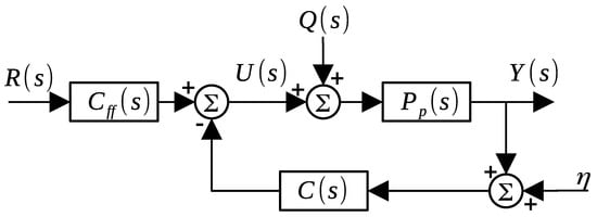
Figure 20.
MSP-PID control structure proposed in [45].
Now consider the delay partition proposed in (21) with and for system (54). Thus, the state-space representation of system (54) without delays and is given by,
Considering that a value of has been selected, a value of is proposed to determine the sampling period, which is calculated as
For the design of the predictor, a state-space discrete representation is obtained from (58), using the sampling period defined in (59). Then, by considering (29), we obtain the corresponding discrete representation (28),
Once these matrices have been determined, the values of the vector G guarantee the stability of . To achieve this, the poles of the characteristic equation are relocated to the positions . The vector G that satisfies these conditions is given by,
Note that the vector G obtained in (61) allows to ensure convergence between the estimated signal and the original signal in the scheme of Figure 8. Using Lemma 1, the values of , , and for the system are used for simulation. Therefore, given by (16) can be written as,
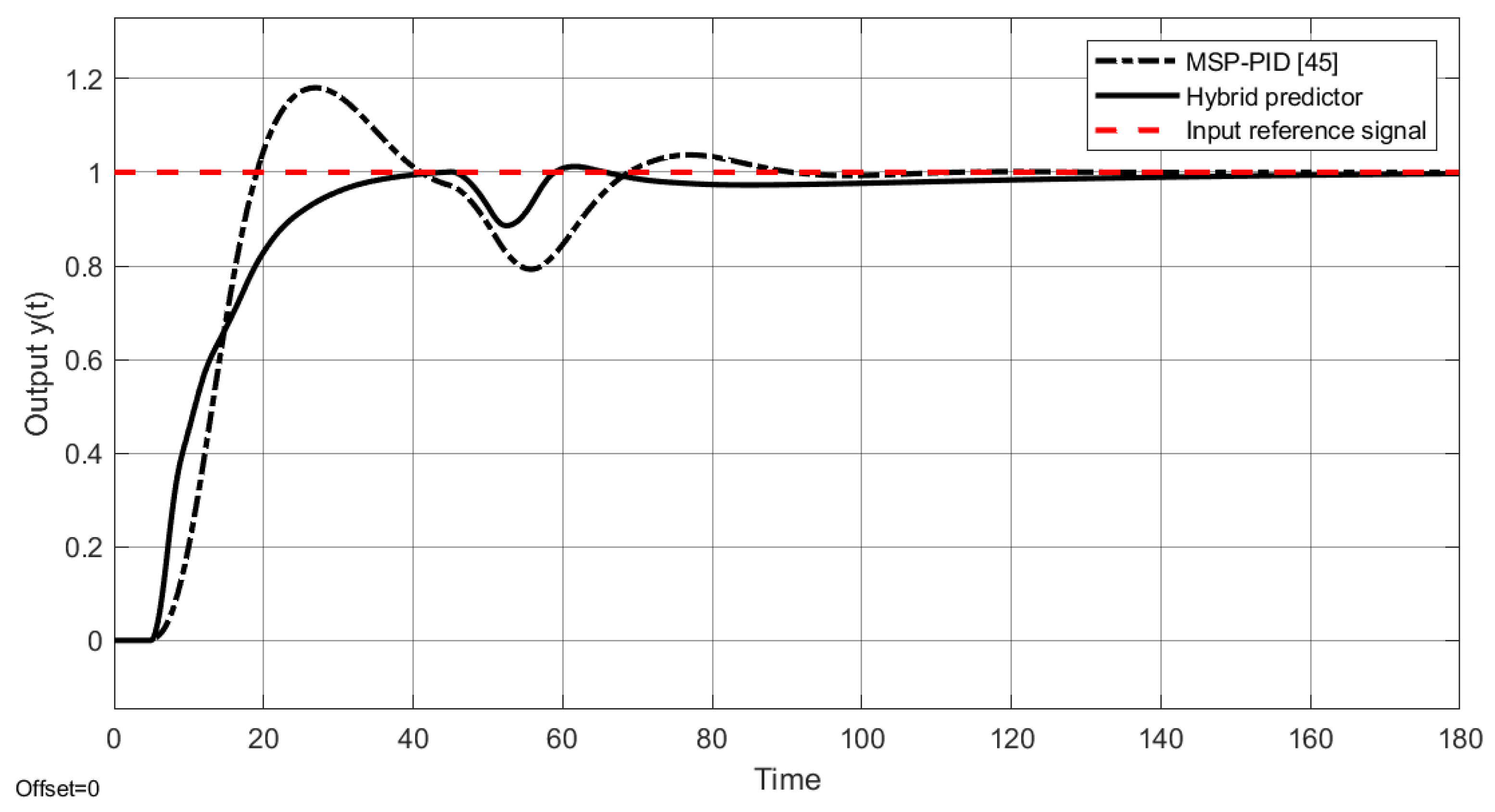
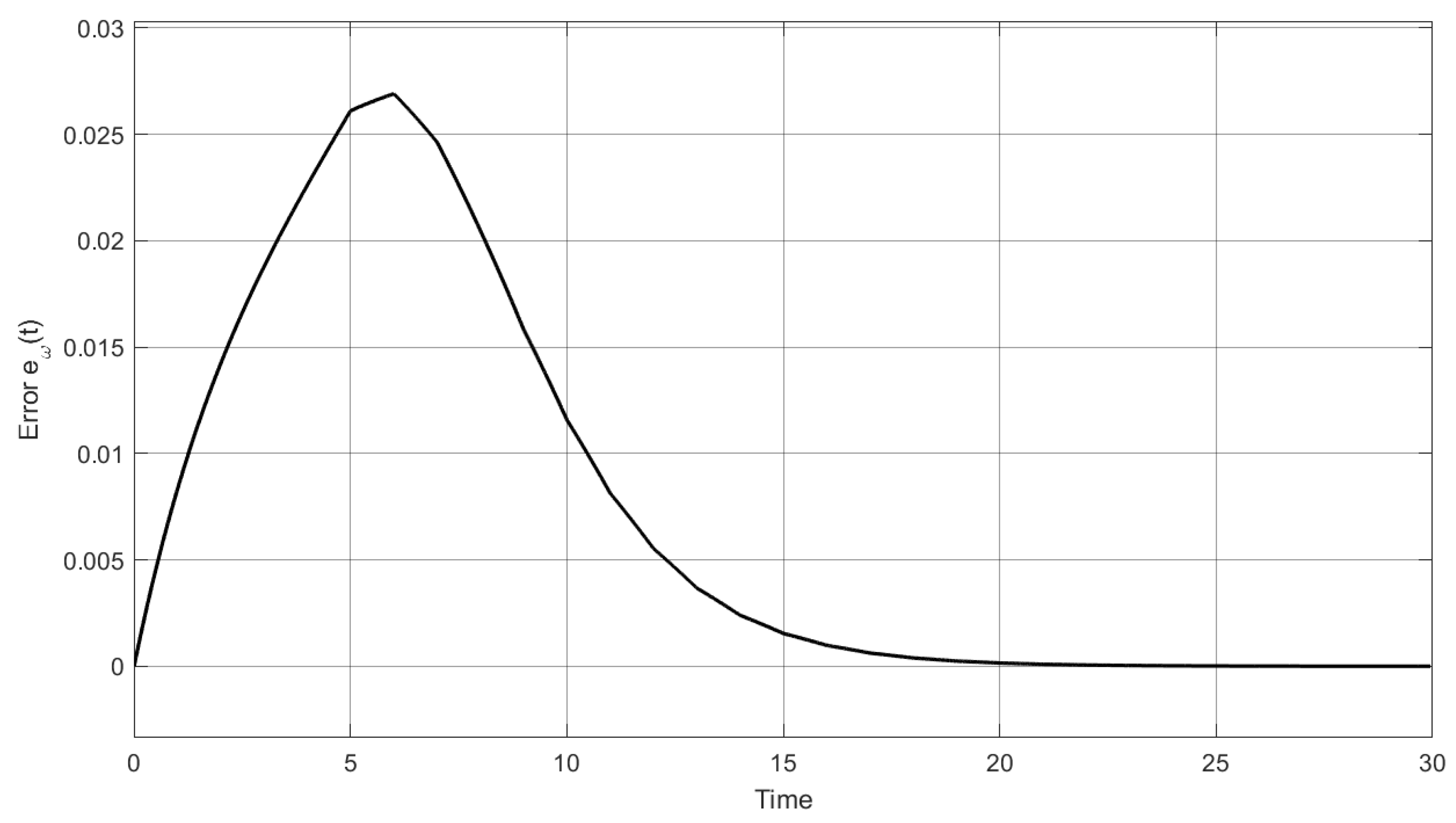
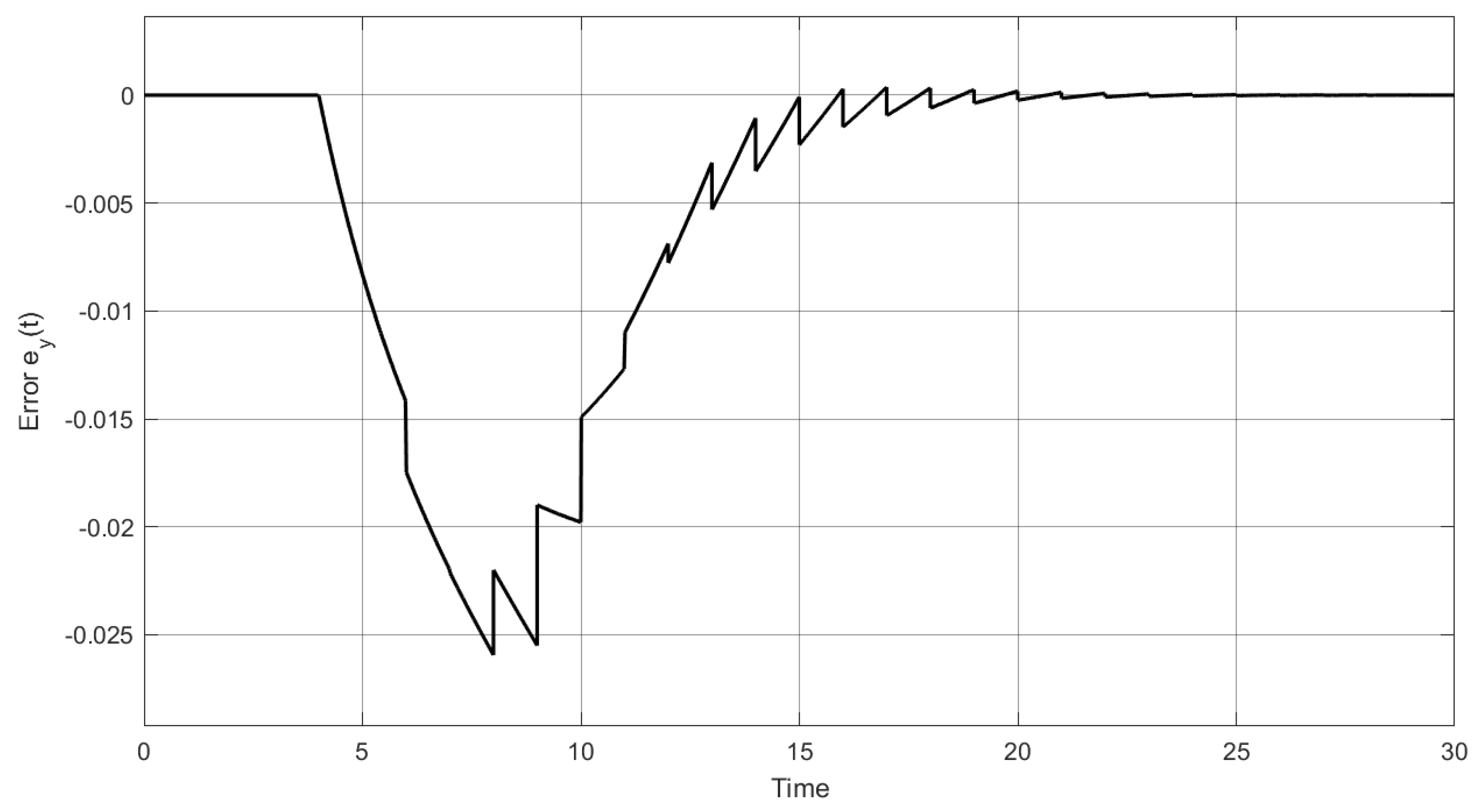
Additionally, to achieve a better transient output response, the controller with two degrees is implemented. This is, with as (44) where and . For the simulation, a step input of amplitude 1 and an initial condition for the unstable pole of are considered. Figure 21 shows the output responses of both control strategies when a disturbances is introduced at s. The results show that both control strategies present stable output responses and are able to reject disturbances. An important aspect in the implementation of the proposed control scheme is that, in order to guarantee the rejection of disturbances, it is required to introduce a gain of in the error signal as . This additional gain is added due to the fact that a large sampling time T, can introduce additional behaviors in the control signal, which degrades the performance of the proposed scheme and reduces its capability to reject disturbances. In Figure 22, the behavior of the strategy reported in [45] and the proposed hybrid–predictor scheme under uncertainties in the plant are shown; the uncertainty is set to the delay size of . The estimation error signals and the system output error signals are presented in Figure 23 and Figure 24, respectively, where both estimation errors tend to zero at finite times illustrating the success of the estimated variables.
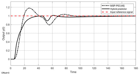
Figure 21.
Output response of the system under an active disturbance s for the Example 3.
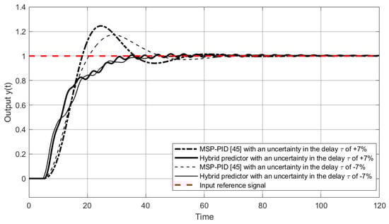
Figure 22.
Output response of the system with uncertainty in the size of the delay in the Example 3.
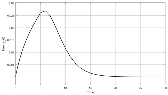
Figure 23.
Output estimation error with initial conditions for Example 3.
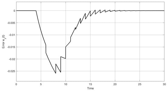
Figure 24.
Output estimation error with initial conditions for Example 3.
Finally, Table 2 shows the results of the evaluation of various performance indicators for both control strategies. This analysis includes two cases: the first one considers the nominal system (54) and the second one considers uncertainty in the delay size of into the nominal system. It is observed that the results of the evaluation of the strategy proposed in this work have better results in the all performance indices for the control signal and for the output signal (nominal values) with respect to the work presented in [45], due to our control proposal presents all indices performance smaller than the indices derived from control strategy [45]. For the case where uncertainties in the delay size are considered, the results show that the proposed hybrid predictor scheme only outperforms [45] in the ITAE index on the control signal . Likewise, for the output signal it is observed that in all performance indices, the proposed strategy has better results with respect to [45].
Table 2.
Comparative table of quantitative evaluation of the two strategies of Example 3.
4.4. Example 4
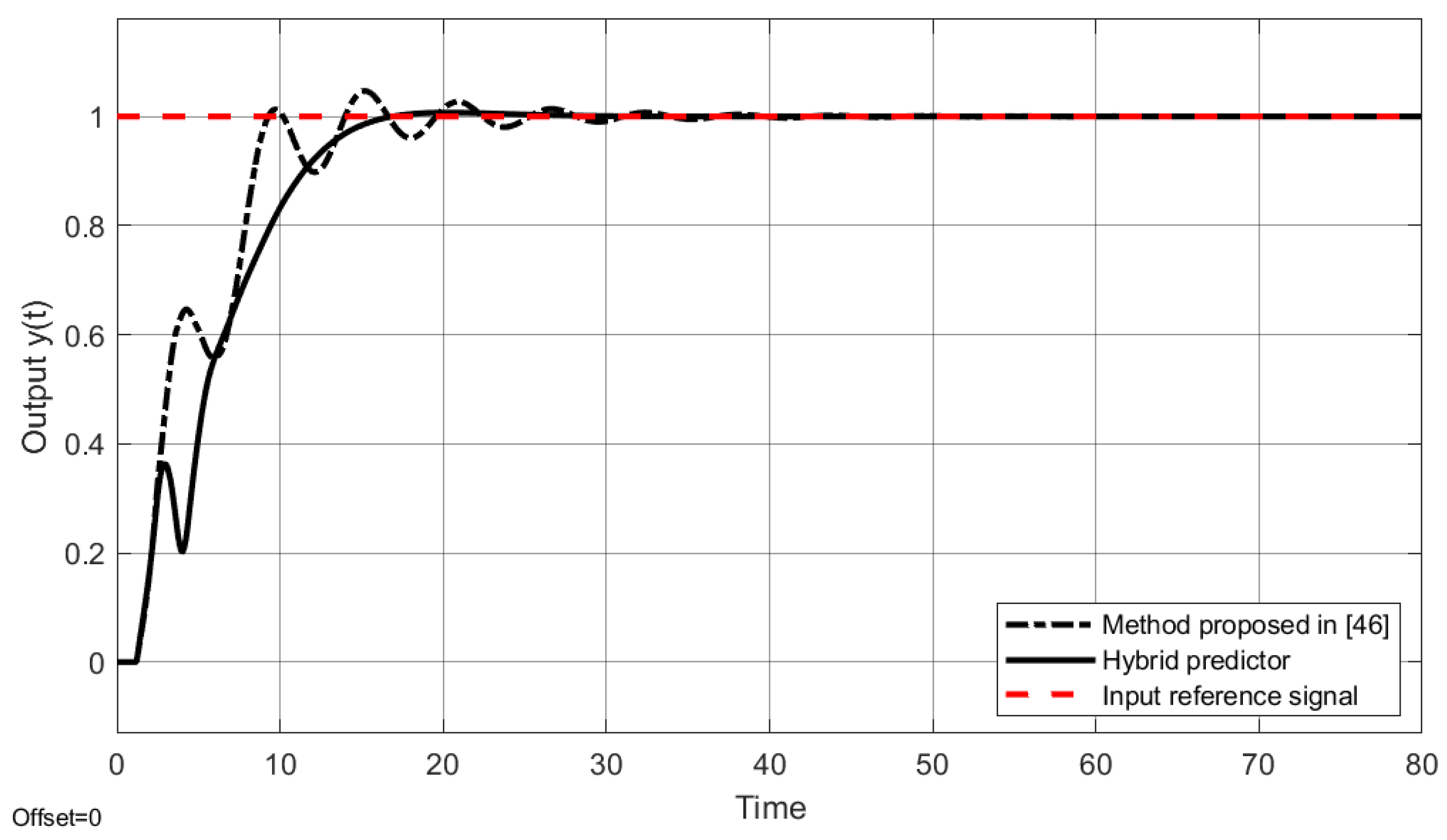
The following example corresponds to an unstable second order process with delay presented in [46], the transfer function is,
In the proposed scheme in [46], a design method based on the direct synthesis approach on a modified SP structure is presented, in the design, an I-PD controller structure, and a cascaded PD controller is used. In the scheme proposed in [46], the following controllers are used,
where , , , , , and . On the other hand, to design the hybrid predictor, we apply the partition (with , ) to the system (63), its delay-free state-space representation is given by
Considering the value selected of , we define as the number of partitions to calculate the sampling period by the expression
The predictor is designed by discretizing the model in state space (65) using (28) and the sampling period , giving the following results:
To achieve the stability of the system , it is required to obtain the values of the vector G. To do this, the poles of the characteristic equation are relocated at . The vector G that satisfies these requirements is expressed by,
For the control given by (16), we design for the system , this is,
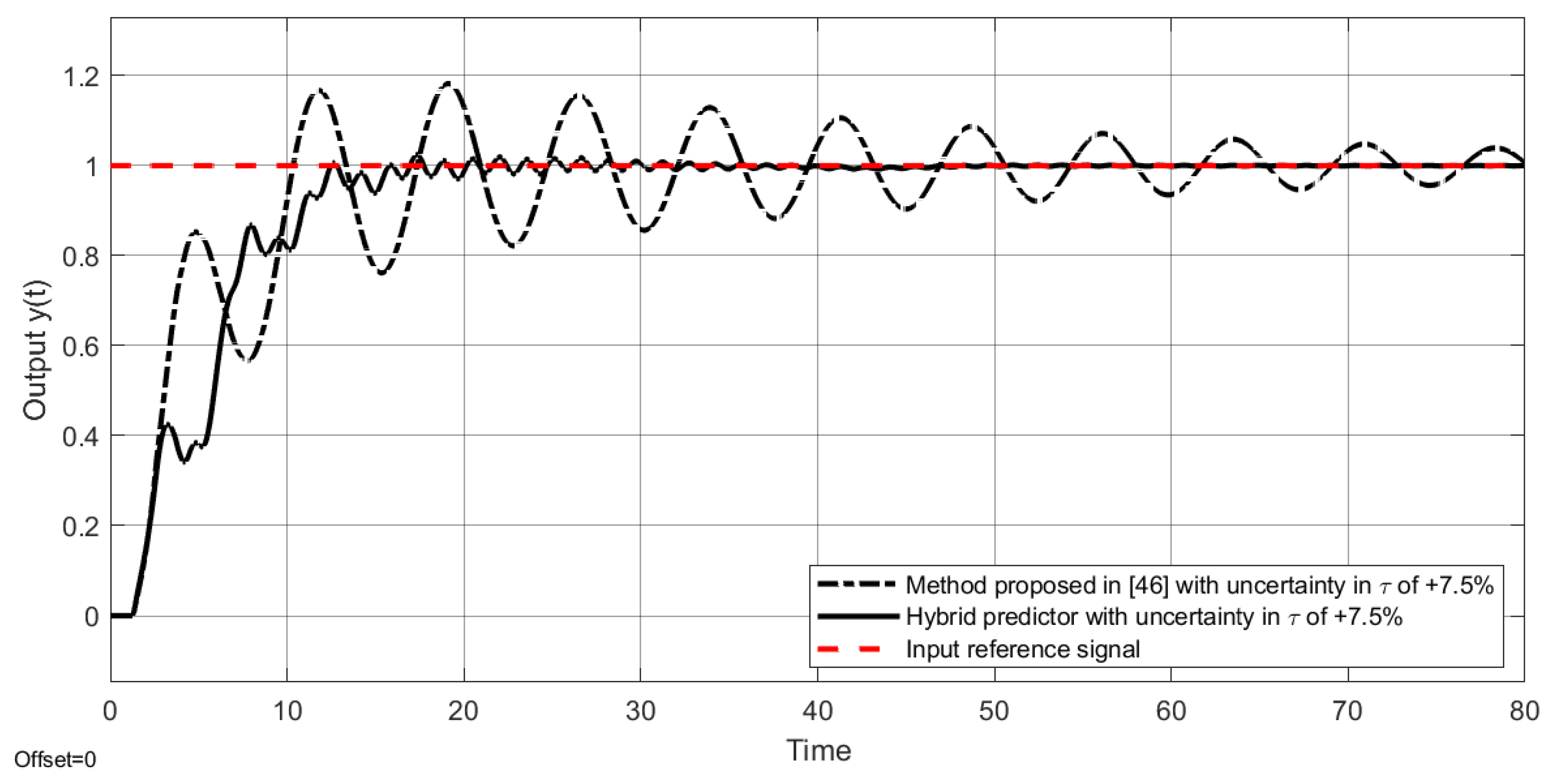
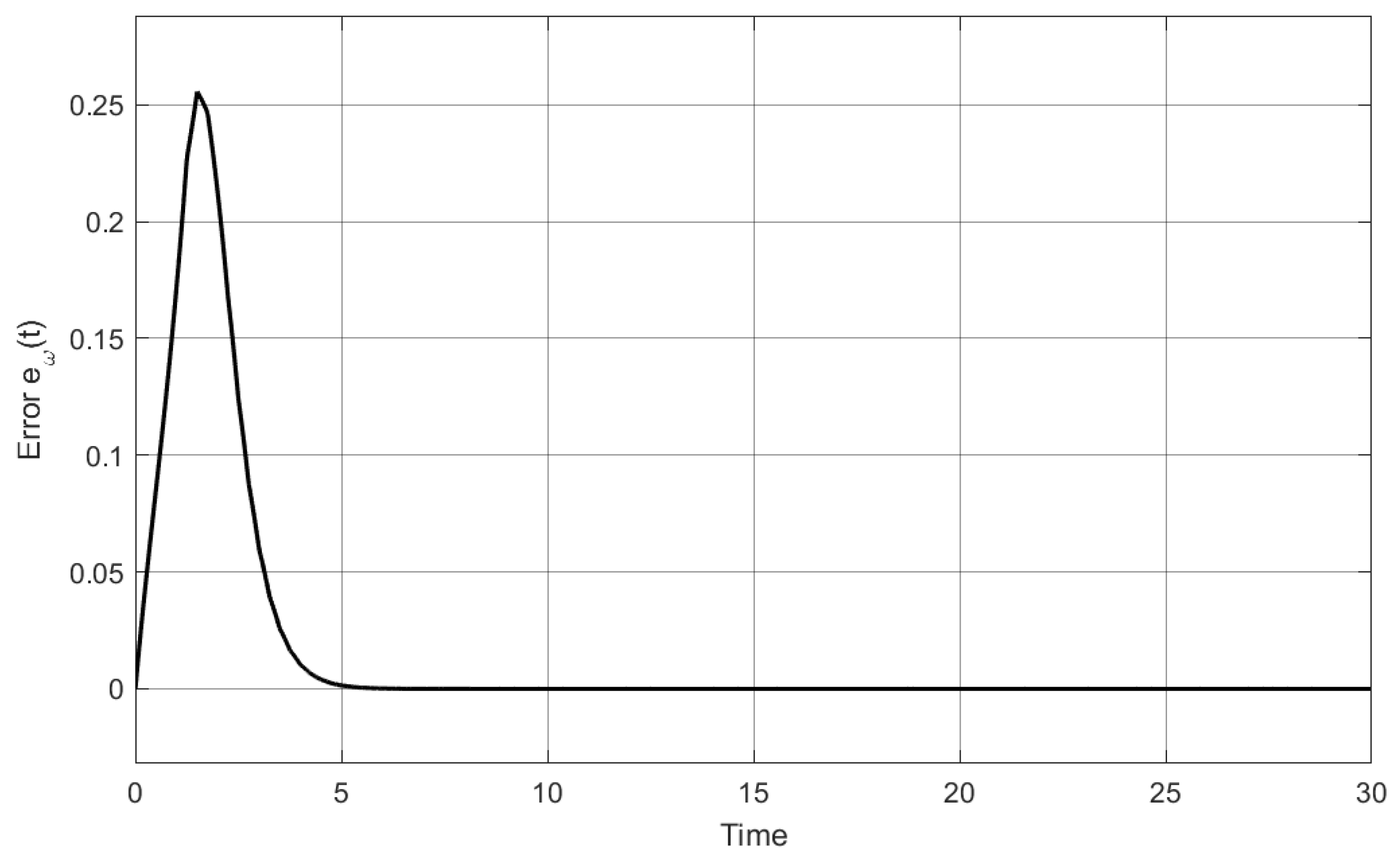
A two-degree-of-freedom PID controller is implemented—this is with as (44) with parameters and . For the simulation, a unit step input and an initial condition of at the unstable pole is considered. Figure 25 shows that both control strategies achieve steady-state stability, but the proposed scheme reduces the time to reach steady state. Likewise, Figure 26 shows the robustness of the method to uncertainties in of , maintaining stability against larger oscillations of the strategy [46], while Figure 27 shows the estimation error signals at initial conditions.
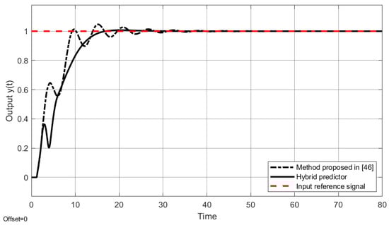
Figure 25.
Output response of the system with initial conditions for Example 4.
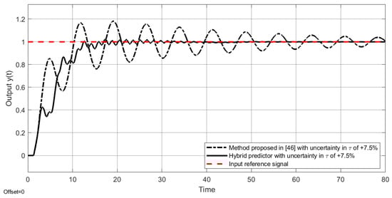
Figure 26.
Output response of the system with uncertainty in for Example 4.
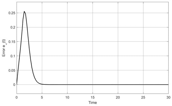
Figure 27.
Output estimation error with initial conditions for Example 4.
Finally, Table 3 shows the results of both control strategies, evaluating the performance indices both in the nominal system (63) as well as the case with uncertainty in . The results show that the strategy proposed in this work offers better performance than [46] in terms of the system output signal , both under nominal conditions and uncertainties in the delay size. Also, it is observed that the results of the strategy proposed in this work present better results in all the performance indices for the control signal when the nominal case is taken into account. Similar results are obtained in both control strategies when the case in which uncertainties in the delay size are considered, the results show that the proposed hybrid predictor scheme only outperforms [46] in the IAE index.
Table 3.
Comparative table of quantitative evaluation of the two strategies of Example 4.
5. Conclusions
In this work, the problem of the stabilization and control of unstable systems of high order and with delay in the direct trajectory is addressed. To solve this problem, a methodology for the design of a hybrid predictor is proposed, in order to estimate the plant state before the delay. This strategy is based on the use of an analogue predictor that is obtained from the discrete injection of the error signal. In this way, an analogue prediction of the internal signals of the plant is obtained. In this work, two-degrees-of-freedom control is used for the control stage, but another type of strategy can be used, such as a strategy that contains an integral-type part. The proposed application of the presented scheme is essentially based on the need to eliminate the restriction when designing the predictor, since sometimes the sampling period T derived from this condition may not be manageable for the design and implementation. Finally, the behaviour of the proposed method is shown through numerical simulations.
Author Contributions
Conceptualization, R.J.V.-G.; Methodology, B.d.M.-C., J.F.M.-R. and A.U.-C.; Validation, B.d.M.-C.; Formal analysis, R.J.V.-G., B.d.M.-C., J.F.M.-R. and A.U.-C.; Investigation, R.J.V.-G., J.F.M.-R. and A.U.-C.; Writing—original draft, R.J.V.-G., B.d.M.-C. and J.F.M.-R.; Writing—review & editing, A.U.-C. All authors have read and agreed to the published version of the manuscript.
Funding
This research received no external funding.
Data Availability Statement
The original contributions presented in this study are included in the article. Further inquiries can be directed to the corresponding author(s).
Conflicts of Interest
The authors declare no conflict of interest.
References
- Ali, E.; Alhumaizi, K. Temperature control of ethylene to butene-1 dimerization reactor. Ind. Eng. Chem. Res. 2000, 39, 1320–1329. [Google Scholar] [CrossRef]
- Chien, Y. The effect of non-ideal mixing on the number of steady states and dynamic behaviour for autocatalytical reactions in a CSTR. Can. J. Chem. Eng. 2001, 79, 112–118. [Google Scholar] [CrossRef]
- Liu, T.; Zhang, W.; Gu, D. Analytical design of two-degree-of-freedom control scheme for open-loop unstable processes with time delay. J. Process. Control. 2005, 15, 559–572. [Google Scholar] [CrossRef]
- Niculescu, S. Delay Effects on Stability: A Robust Control Approach; Springer: Berlin, Germany, 2001. [Google Scholar]
- Rao, A.S.; Chidambaram, M. PI/PID controllers design for integrating and unstable systems. In PID Control in the Third Millennium; Advances in Industrial Control; Vilanova, R., Visioli, A., Eds.; Springer: London, UK, 2012. [Google Scholar]
- Ailon, A.; Gil’, M.I. Stability analysis of a rigid robot with output-based controller and time delay. Syst. Control Lett. 2000, 40, 31–35. [Google Scholar] [CrossRef]
- Liu, T.; Cai, Y.; Gu, D.; Zhang, W. New modified Smith predictor scheme for integrating and unstable processes with time delay. Iee Proc.-Control Theory Appl. 2005, 152, 238–246. [Google Scholar] [CrossRef]
- Steinberger, M.; Horn, M. Robust filtered Smith predictors for networked control systems with packet-based data transmission. J. Process. Control 2022, 111, 86–96. [Google Scholar] [CrossRef]
- Smith, O. Closer control of loops with dead time. Chem. Eng. Prog. 1957, 53, 217–219. [Google Scholar]
- Rao, A.S.; Chidambaram, M. Enhanced Smith predictor for unstable processes with time delay. Ind. Eng. Chem. Res. 2005, 44, 8291–8299. [Google Scholar] [CrossRef]
- Márquez-Rubio, J.F.; Del-Muro-Cuéllar, B.; Velasco-Villa, M.; Novella-Rodríguez, D.F. Observer–PID stabilization strategy for unstable first-order linear systems with large time delay. Ind. Eng. Chem. Res. 2012, 51, 8477–8487. [Google Scholar] [CrossRef]
- Rubio, J.F.; Cuéllar, B.D.; Villa, M.V.; Ramírez, J.Á. An improved sufficient condition for stabilisation of unstable first-order processes by observer-state feedback. Int. J. Control 2015, 88, 403–412. [Google Scholar] [CrossRef]
- Del-Muro-Cuéllar, B.; Velasco-Villa, M.; Márquez-Rubio, J.F.; Álvarez-Ramírez, J.D. On the control of unstable first order linear systems with large time lag: Observer based approach. Eur. J. Control 2012, 18, 439–451. [Google Scholar] [CrossRef]
- Babu, D.; Kumar, D.B.; Sree, R.P. Tuning of PID controllers for unstable systems using direct synthesis method. Indian Chem. Eng. 2017, 59, 215–241. [Google Scholar] [CrossRef]
- Kishore, C.R.; Sree, R.P. Design of PID controllers for unstable systems using multiple dominant poleplacement method. Indian Chem. Eng. 2018, 60, 356–370. [Google Scholar] [CrossRef]
- Alyoussef, F.; Kaya, I. Simple PI-PD tuning rules based on the centroid of the stability region for controlling unstable and integrating processes. ISA Trans. 2022, 134, 238–255. [Google Scholar] [CrossRef]
- Hernández-Pérez, M.A.; Muro-Cuéllar, B.D.; Velasco-Villa, M. PID for the stabilization of high-order unstable delayed systems with possible complex conjugate poles. Asia-Pac. J. Chem. Eng. 2015, 10, 687–699. [Google Scholar] [CrossRef]
- del Muro-Cuéllar, B.; Vazquez-Guerra, R.J.; Márquez-Rubio, J.F. Digital two-degree-of-freedom controller for processes with large time-delay. Stud. Inform. Control 2020, 29, 17–24. [Google Scholar] [CrossRef]
- Kumar, D.; Padma Sree, R. Tuning of IMC based PID controllers for integrating systems with time delay. ISA Trans. 2016, 63, 242–255. [Google Scholar] [CrossRef]
- Barragan-Bonilla, L.A.; Márquez-Rubio, J.F.; del Muro Cuellar, B.; Vázquez-Guerra, R.J.; Martínez, C. Observer-based control for high order delayed systems with an unstable pole and a pole at the origin. Asian J. Control 2022, 25, 1759–1774. [Google Scholar] [CrossRef]
- Karan, S.; Dey, C.; Mukherjee, S. Simple internal model control based modified Smith predictor for integrating time delayed processes with real-time verification. ISA Trans. 2021, 121, 240–257. [Google Scholar] [CrossRef]
- Lee, S.C.; Wang, Q.; Xiang, C. Stabilization of all-pole unstable delay processes by simple controllers. J. Process. Control 2010, 20, 235–239. [Google Scholar] [CrossRef]
- Cho, W.; Lee, J.; Edgar, T.F. Simple analytic proportional-integral-derivative (PID) controller tuning rules for unstable processes. Ind. Eng. Chem. Res. 2014, 53, 5048–5054. [Google Scholar] [CrossRef]
- Márquez-Rubio, J.F.; del Muro-Cuéllar, B.; Barragan-Bonilla, L.A.; Vázquez-Guerra, R.J.; Urquiza-Castro, A. Control for a class of unstable high-order systems with time delay based on observer–predictor approach. Processes 2023, 11, 1613. [Google Scholar] [CrossRef]
- Tognetti, E.S.; de Oliveira, G.A. Robust state feedback-based design of PID controllers for high-order systems with time-delay and parametric uncertainties. J. Control. Autom. Electr. Syst. 2022, 33, 382–392. [Google Scholar] [CrossRef]
- Acharya, D.; Swain, S.K.; Mishra, S.K. Real-time implementation of a stable 2 DOF PID controller for unstable second-order magnetic levitation system with time delay. Arab. J. Sci. Eng. 2020, 45, 6311–6329. [Google Scholar] [CrossRef]
- Novella-Rodríguez, D.F.; Tudón-Martínez, J.C.; Vázquez-Guerra, R.J.; Márquez-Rubio, J.F. Feedback control based on a sequential observer-predictor for systems with unknown actuator delay. Int. J. Control. Autom. Syst. 2022, 20, 2779–2791. [Google Scholar] [CrossRef]
- Bobál, V.; Kubalcik, M.; Dostál, P.; Matejicek, J. Adaptive predictive control of time-delay systems. Comput. Math. Appl. 2013, 66, 165–176. [Google Scholar] [CrossRef]
- Rivas-Perez, R.; Feliu-Batlle, V.; Castillo-García, F.J.; Sánchez-Rodríguez, L.; Linares-Saez, A. Robust fractional order controller implemented in the first pool of the Imperial de Aragón main canal. Tecnol. Cienc. Agua 2014, 5, 23–42. [Google Scholar]
- Jin, Q.; Hao, F.; Wang, Q. A multivariable IMC-PID method for non-square large time delay systems using NPSO algorithm. J. Process. Control 2013, 23, 649–663. [Google Scholar] [CrossRef]
- Márquez-Rubio, J.F.; del Muro-Cuéllar, B.; Vázquez-Guerra, R.J.; Urquiza-Castro, A.; Barragan-Bonilla, L.A.; Martínez, C. A simple modification to the Smith predictor structure for dealing with high-order delayed processes considering one unstable pole. J. Process. Control 2024, 142, 103299. [Google Scholar] [CrossRef]
- Garcia, P.C.; Albertos, P. Robust tuning of a generalized predictor-based controller for integrating and unstable systems with long time-delay. J. Process. Control 2013, 23, 1205–1216. [Google Scholar] [CrossRef]
- Buenfil-Hernández, R.; Del-Muro-Cuéllar, B. Predictor híbrido para sistemas lineales con retardo de tiempo. AMCA 2013, 2013, 111–116. [Google Scholar]
- Rao, A.S.; Rao, V.S.; Chidambaram, M. Simple analytical design of modified Smith predictor with improved performance for unstable first-order plus time delay (FOPTD) processes. Ind. Eng. Chem. Res. 2007, 46, 4561–4571. [Google Scholar] [CrossRef]
- Sanz, R.; Garcia, P.C.; Albertos, P. A generalized Smith predictor for unstable time-delay SISO systems. ISA Trans. 2017, 72, 197–204. [Google Scholar] [CrossRef]
- Torrico, B.C.; Pereira, R.D.; Sombra, A.K.; Nogueira, F.G. Simplified filtered Smith predictor for high-order dead-time processes. ISA Trans. 2020, 109, 11–21. [Google Scholar] [CrossRef] [PubMed]
- Garcia, P.C.; Albertos, P.; Hägglund, T. Control of unstable non-minimum-phase delayed systems. J. Process. Control 2006, 16, 1099–1111. [Google Scholar] [CrossRef]
- Albertos, P.; Garcia, P.C. Robust control design for long time-delay systems. J. Process. Control 2009, 19, 1640–1648. [Google Scholar] [CrossRef]
- Normey-Rico, J.E.; Camacho, E.F. Unified approach for robust dead-time compensator design. J. Process. Control 2009, 19, 38–47. [Google Scholar] [CrossRef]
- Normey-Rico, J.E.; Camacho, E.F. Simple robust dead-time compensator for first-order plus dead-time unstable processes. Ind. Eng. Chem. Res. 2008, 47, 4784–4790. [Google Scholar] [CrossRef]
- Santos, T.L.; Botura, P.E.; Normey-Rico, J.E. Dealing with noise in unstable dead-time process control. J. Process. Control 2010, 20, 840–847. [Google Scholar] [CrossRef]
- Ogata, K. Sistemas de Control en Tiempo Discreto; Pearson Educación: Estado de Mexico, Mexico, 1996. [Google Scholar]
- Åström, K.J.; Hägglund, T. PID Controllers: Theory, Design and Tuning; Instrument Society of America: Research Triangle Park, NC, USA, 1995. [Google Scholar]
- Wang, Y. Determination of all feasible robust PID controllers for open-loop unstable plus time delay processes with gain margin and phase margin specifications. ISA Trans. 2014, 53, 628–646. [Google Scholar] [CrossRef]
- Matausek, M.R.; Ribic, A.I. Control of stable, integrating and unstable processes by the Modified Smith Predictor. J. Process. Control 2012, 22, 338–343. [Google Scholar] [CrossRef]
- İçmez, Y.; Can, M.S. Smith Predictor Controller Design Using the Direct Synthesis Method for Unstable Second-Order and Time-Delay Systems. Processes 2023, 11, 941. [Google Scholar] [CrossRef]


Disclaimer/Publisher’s Note: The statements, opinions and data contained in all publications are solely those of the individual author(s) and contributor(s) and not of MDPI and/or the editor(s). MDPI and/or the editor(s) disclaim responsibility for any injury to people or property resulting from any ideas, methods, instructions or products referred to in the content. |
© 2025 by the authors. Licensee MDPI, Basel, Switzerland. This article is an open access article distributed under the terms and conditions of the Creative Commons Attribution (CC BY) license (https://creativecommons.org/licenses/by/4.0/).