Optimisation for Sustainable Supply Chain of Aviation Fuel, Green Diesel, and Gasoline from Microalgae Cultivated in Sugarcane Vinasse

Abstract

The development of new technologies for the production of renewable energy is fundamental to reducing greenhouse gas emissions. Therefore, the search for new energy generation methods that are environmentally responsible, socially rational, and economically viable is gaining momentum in order to mitigate carbon footprint. The aviation sector is responsible for a significant fraction of greenhouse gas emissions; for this reason, the decarbonisation of this sector must be investigated using biorefinery models. This study presents a mixed-integer linear programming (MILP) model for optimising the design and configuration of the supply chain in different states of Brazil for the production of sustainable aviation fuel (SAF) and green diesel and gasoline, using microalgae cultivated in sugarcane vinasse as the raw material. The technology of hydrothermal liquefaction was assessed in terms of its capacity to convert microalgae without need for the energy-intensive drying step. The MILP model was developed in the LINGO v.20 software using a library of physical and economic process models. We consider the selection of processes based on the object of total minimum cost, with optimal production plant scaling and regional supply chain design, including an assessment of resources and final product distribution. A case study was implemented in Brazil, considering different regions of the country and its local demands for fuels. São Paulo is the most profitable state, with a cash flow of 1071.09 and an IRR of 36.19%, far outperforming the rest. Transport emissions alone represent between 0.6 and 8.6% of emissions generated by the model. The costs of raw materials, mainly hydrogen (57%) and electricity (27%) represent the main costs evaluated in the model. The production cost (MUS$/TJ biofuel) is in the range of 0.009–0.011. Finally, changes in the cost of electricity have the greatest impact on the model.

1. Introduction

The depletion of fossil fuels, waste generation, increasing energy demands, and cli-mate change mitigation have raised concerns about sustainable and renewable energy pro-duction [1,2], and the energy transition will help in proper waste management and the development of a green economy [3]. Biomass (referring to those organic materials that can be converted into useful energy) is a green and sustainable renewable resource [4]. About 89% of biomass is used as heat in combustion, 7% is used as transportation fuel, and 4% is used to produce electricity [5]. Renewable energies such as biomass fuel (biofuels) have high potential to replace fossil fuels, [6] and have the advantage of being renewable sources of carbon [7]. Biofuels include liquid (biodiesel, bioethanol, bio-oil), solid (biochar, pellets), and gaseous (biogas, syngas) fuels and can be used to generate power and heat, or as a transportation fuel [3,6]. Biofuels are obtained through the conversion of biomass, which includes algae biomass, animal residues, wastes, and lignocellulosic biomass. Depending on their feedstock, nature, and properties, the biofuels produced from them can be divided into four categories: first-, second-, third-, and fourth-generation fuels [8,9,10].

Sugarcane is one of the main crops worldwide and Brazil is its largest producer, fol-lowed by India, China, and Thailand [11]. Sugarcane is mainly used for the production of sugar and alcohol. However, an important by-product of the sugarcane industry is bagasse, a fibrous material that is used as a raw material for renewable energy production [12]. In addition to bagasse, vinasse is another by-product of the sugarcane industry that can be used for energy generation [13]. It is estimated that for every litre of ethanol, be-tween 10 and 14 L of vinasse are produced [14,15]. This by-product has a high organic content; therefore, it is not advisable to dispose of it in water bodies. Among its main uses, vinasse has potential for biogas production through anaerobic digestion [1,16] and can also be used as a culture medium for the production of microalgae biomass [17].

Microalgae are microorganisms that use sunlight and carbon dioxide to generate chemical energy while producing oxygen, i.e., they store the sun’s energy in the form of organic compounds such as carbohydrates, lipids, and proteins. These compounds can then be used as a source of energy or feedstock for biofuels [18,19,20]. They are considered as fundamental sources of biomass for biofuel production because of their enormous benefits: (1) they can be cultivated in fresh and salt water; (2) they display high growth and production rates compared to other plants; (3) they require less water consumption for growth than terrestrial crops; and (4) cultivation is possible in the absence of terrestrial soil [21]. These types of microorganisms are used in various fields such as agriculture, food, medicine, and cosmetics [22]. In this sense, due to the energy, environmental, and economic crisis, microalgae biomass biorefineries represent a potential viable solution to this crisis. Therefore, one way to valorise the different sugarcane by-products is through the development of biorefineries to produce biochemicals and/or profitable biofuels [23]. Brazil is one of the pioneer countries in the biofuels market and its biorefinery infrastructure is a base for the implementation of various methodologies linked to large-scale biofuel production [24,25]. The term biorefinery encompasses networks of facilities that integrate different processes and equipment to transform biomass into biofuels, biomaterials, and biochemicals [26]. Biorefineries play an important role in industries because they can efficiently use resources, offer a solution to climate change, can reduce dependence on fossil fuels, and can meet energy needs [27]. The main obstacle when evaluating biorefineries projects is technical and economic feasibility; therefore, it is essential to address the integration of mass and energy flows through mathematical models for resource optimisation [23]. The optimisation of superstructures based on mathematical models provides a versatile array of configurations for a defined objective function [28]; thus, different conversion routes, multiple feedstocks, multiple periods, and the production of various biofuels can be included [29]. Another important aspect when evaluating the economic part of a biorefinery is to consider the environmental dimension and to analyse the supply chain. A supply chain is a network used to coordinate feedstock availability and product demand [30], and its proper design can provide a highly reliable and cost-effective system [31].

Several studies have evaluated the optimisation of superstructures using linear or mixed-integer nonlinear integer linear programming (MILP or MINLP) to integrate feed-stock streams, exploit waste, and produce a variety of biofuels and high-value products through the biorefinery concept. Varshney et al. [32] formulated an optimisation model for the production of bioethanol, pellets, and electricity from bagasse processing with the objectives of maximising net present value (NPV) and minimising greenhouse gas emissions and water footprint. Macowski et al. [33] developed a mixed-integer linear programming (MILP) model to optimise the supply chain for the production of bioethanol from sugarcane to evaluate the environmental impact and economic value.

Gutierrez-Franco et al. [34] proposed the use of a multi-objective (economic, environmental and social) model (MILP) to design a sustainable supply chain for biofuels in Colombia from forest residues. Moretti et al. [35] formulated a model (MILP) to minimise the fuel production costs of a supply chain in Italy from 3 different feedstocks (wood chips, grape pomace, and olive pomace), 2 means of transportation (train and truck), and possible feedstock pre-processing. Gilani and Sahebi [36] proposed a model (MILP) of the supply chain for biofuel production from sugarcane with the objective of maximising profits from sales, minimising environmental impacts, and maximising supply chain employment. Basile et al. [37] applied an economic and environmental optimisation model for the design of a supply chain in Sweden for the production of biomethanol from forest residues. Vitale et al. [38] proposed a model for the supply chain in Argentina, using wood waste and forest residues as raw material for the production of wood pellets, with the objective of minimising the operating cost. Infante et al. [39] developed a mixed-integer linear programming (MILP) model to minimise the carbon dioxide balance in the evaluation of a microalgae biorefinery, considering the production of various biofuels in Colombia. The results showed that producing diesel and green gasoline via hydrothermal liquefaction was the most favourable conversion pathway for minimising carbon dioxide emissions. Bagasse is also used as fuel for power and heat systems and as a pellet product. Loon et al. [40] studied a MILP model for the conversion of oil palm biomass into bio-based products and electricity. The results indicated that 0.2271 GWh/year of electricity and 0.0050636 Mtonnes of biofertilizers could be generated. Jabbarzadeh and Shamsi [41] proposed an optimisation model for the design and planning of a supply chain dedicated to bioethanol production from second- and third-generation biomass. Eslamipoor [42] discussed the importance of reducing carbon emissions in a sustainable supply chain (SSC) through carbon pricing. The results showed that a decentralised supply chain tends to be inefficient in terms of coordination, because the benefits are mainly concentrated to the retailer, while the producer barely covers its costs, without making a profit.

This study proposes the application of a mixed-integer linear programming (MILP) model for the optimisation of biorefineries by studying the operating conditions of a supply chain that uses sugarcane vinasse as a microalgae culture medium for the production of sustainable aviation fuel and green diesel and gasoline in different states of Brazil. We analyse the model from both economic and environmental perspectives.

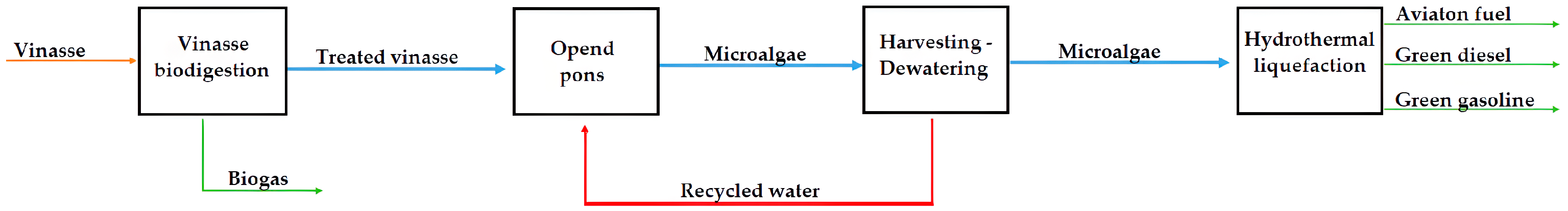
2. Materials and Methods

The optimisation of the superstructure consists of devising a mathematical formulation based on the biorefinery’s objectives. A mixed-integer linear programming (MILP) model based on superstructure optimisation is developed for the production of SAF and green diesel and gasoline from an integrated microalgae biorefinery, using vinasse as the culture medium. The methodology used is based on three main steps. (1) We develop a superstructure of production processes steps, taking into account secondary data. (2) We formulate mathematical physical and economical models for mass and energy balance as well as the capital and operating costs associated with each model. (3) We solve the mathematical model to evaluate the objective function proposed.

The developed superstructure consists of different main processing steps/stages: (1) vinasse biodigestion, (2) microalgae cultivation in open ponds, (3) harvesting and dewatering, and (4) the conversion of microalgae biomass into final biofuels by hydrothermal liquefaction and upgrade. All of the above steps/stages are required for each constituent unit of the system being evaluated. Figure 1 shows a representation of all the steps/stages that make up the biorefinery.

Vinasse biodigestion: In order to calculate the available vinasse, we evaluated the ethanol production capacities of the states addressed in the study. For each litre of ethanol produced, 13.82 litres of vinasse are produced [43]. The produced vinasse is fed into an anaerobic biodigester to produce biogas, a compound mainly composed of methane (CH₄), carbon dioxide (CO₂) and hydrogen sulphide (H₂S). Using the volume of vinasse produced in each state and the typical Chemical Oxygen Demand (COD) of the vinasse, the total COD load can be defined. Based on the removal efficiency of the UASB reactor (treatment method chosen for this study), the amount of COD removed can be calculated and the biogas flow rate of the system can be calculated. In this unit, biodigested vinasse not only produces biogas but also serves as a culture medium for microalgae. Key parameters include vinasse COD value = 33.25 kg/m³ [44]; UASB reactor efficiency = 62.5% [44,45]; CH₄ percentage in biogas = 60%; and biogas production per COD removal = 0.234 m³/kg (in terms of CH₄) [45].

Microalgae cultivation (open pond): Open-pond cultivation was chosen for the production of microalgae biomass in this study. We used biodigested diluted vinasse as the culture medium, with a reference vinasse concentration of 5% by volume. The amount of water lost through evaporation depends on factors like climate, temperature, and humidity. According to Guieysse et al. [46], water loss is approximately 0.476 m³/m²/year. The culture system presented a depth of 0.3 m and the system was assumed to be a high-rate algae pond (HRAP) with a constant concentration of 0.56 g/L during harvest periods and a hydraulic retention time of 8 days, corresponding to a biomass productivity of 70 mg/L-day (dry algae base without ash) [47]. The electricity consumption of the paddle wheel and pumps for the cultivation system is 2.7 kW/ha and 0.5 kW/ha, respectively [48].

Harvesting and dewatering: In this study, the harvesting and dewatering of the biomass were carried out in 3 processes: decantation, flocculation, and centrifugation. In the first process, excess water was removed to increase the algae concentration from 0.56 g/L to 20 g/L [49]. The efficiency of this unit was 95%. Subsequently, the microalgae biomass went through a chemical flocculation process to increase the algae concentration to 7.5% by weight. In a flocculation tank, 0.15 g/L of aluminium sulphate was added [50]. The biomass recovery in this process was 98% and the energy consumption was 0.15 kWh/m³ feed [51]. The biomass suspension after flocculation was concentrated by centrifugation at 200 g/L. The cell recovery efficiency was 99% [51].

Hydrothermal liquefaction: After the centrifugation process, the microalgae biomass with 20% solids is used in a hydrothermal liquefaction process for the production of SAF and green diesel and gasoline. During this unit, the main parameters are hydrogen consumption = 0.021 t H₂/t dry microalgae; heat consumption = 0.59 MWh/t dry microalgae; electricity consumption = 0.035 MWh/t dry microalgae; gasoline production = 0.06 t gasoline/t dry microalgae; diesel production = 0.1287 t diesel/t dry microalgae; and SAF production = 0.0924 t SAF/t dry microalgae [52,53].

The biogas produced from the biodigestion of vinasse goes to a purification unit. The purification unit consists of a treatment process that upgrades and enriches the methane in the biogas to produce biomethane. In this study, pressure swing adsorption (PSA) technology is employed to produce biomethane with 99% purity. The energy consumption of this unit is 0.31 kWh/Nm³ of biogas fed, with a CO₂ removal efficiency of 99% and methane losses estimated at 3.5% [54].

For this study, the electricity supply is provided by the available electricity grid.

3. Structure, Formulation and Data of the Model

The optimisation model is a mixed linear programming problem (MILP) based on the superstructure shown in Figure 1. All processes considered in the superstructure are physical models based on the mass balance and energy of each technology, taking into account literature data and estimated data as previously mentioned. The superstructure was modelled as an MILP model and implemented in the LINGO v.20 software. Figure 2 shows a representation of the workflow of the optimisation superstructure. The mathematical model utilized during the case study uses [55,56] for reference.

3.1. Definition of Set

The formulation of the model considers different sets, to include and exclude different processes and parameters. Different main sets are worked on: resource (R), modal (M), location (L), and unit (U). The resource (R) elements are anything that can be transported as consumed resources, intermediates, and final products; the unit (U) elements are any technology that can transform one resource into another. For example, sugarcane vinasse can produce biogas through the biodigestion process. In this case, each element is inserted into the superstructure together with input flows (IAR_u,r) and output flows (OAR_u,r). The elements of the location (L) set represent the places with availability of raw material and/or demand, while the elements of the modal set represent the different modes of transport considered in the model.

3.2. Investment Cost Updating and Linearization

The investment cost is defined as the initial capital expenditure needed to build the biorefinery’s process units, with costs expressed on a per-process-unit basis. When calculating the required investment for plant and unit construction, data from the literature, where unit capacities are known, were used for reference. Since unit costs fluctuate over time, the cost values were adjusted using the Chemical Engineering Plant Cost Index (CEPCI).

In the current study, exponent values of 0.6 were assumed for all units. Since each unit inserted into the superstructure has a reference scale, each capital investment cost at the reference scale must be adjusted. Therefore, a piecewise linearization of the capital cost function was performed for each process. To perform this linearization, the cost curve was obtained as a function of the scale variable (w_u) when using Equation (1), where se is a scale exponent, C_u,p is the adjusted investment cost for the unit, and the investment cost at the reference scale is represented by C0u. The curve is then divided into different levels limited by a minimum and maximum value, CapMin_u,l and CapMax_u,l, respectively. The coefficients of the linearized cost curve for each process are presented in the Supplementary Materials (Table S1).

$${\mathrm{C}}_{\mathrm{u}}{=\mathrm{C}0}_{\mathrm{u}}{\mathrm{w}}_{\mathrm{u}}^{\mathrm{se}}$$

(1)

3.3. Unit Selection and Scaling Adjustment

Selection and scaling for each unit element are performed using Equation (2), where CapMin_u and CapMax_u are minimum and maximum parameters, representing the scaling that a unit can have, y_u,p is a binary variable, representing the existence of that unit, and w_u,p is a continuous variable responsible for unit scaling. When selected, a unit has a y_u,p equal to one, and its w_u,p is limited by CapMin_u and CapMax_u. If not selected, the value zero is assumed, resulting in a w_u,p equal to zero.

$${\mathrm{CapMin}}_{\mathrm{u}}{\mathrm{y}}_{\mathrm{u},\mathrm{p}}\le {\mathrm{w}}_{\mathrm{u},\mathrm{p}}\le {\mathrm{CapMax}}_{\mathrm{u}}{\mathrm{y}}_{\mathrm{u},\mathrm{p}}$$

(2)

When a unit is selected and scaled, one of the levels must also be selected. Only one level is chosen per unit at each location when using Equation (3). If a level is not selected, its binary variables (yl_u,l) will have a value of zero, so the local scale factor variable wl_u,l will also have a value of zero. As such, Equation (4) ensures that w_u will be equal to the value of wl_u,l of the selected level.

$${\displaystyle \sum }_l{\mathrm{yl}}_{\mathrm{u},\mathrm{l}}\le 1$$

(3)

$${\displaystyle \sum }_{\mathrm{l}}{\mathrm{wl}}_{\mathrm{u},\mathrm{l}}{=\mathrm{w}}_{\mathrm{u}}$$

(4)

3.4. Objective Function

The objective function of the superstructure is to minimise total costs, taking into account annualised investment, resource and transportation costs, and the sale of services, as shown in Equation (5).

$$Min \left[INVC+OPEC+RMAC+TRNC-PRSC\right]$$

(5)

Equation (6) was used to calculate the annualised investment cost (INVC), where au,l and bu,l represent the angular and linear coefficients of each linearized interval, respectively. The annualisation factor (AF) was set as 0.072.

$$\mathrm{INVC}={\displaystyle \sum }_{\mathrm{l}}({\mathrm{a}}_{\mathrm{u},\mathrm{l}}{\mathrm{wl}}_{\mathrm{u},\mathrm{l}}{+\mathrm{b}}_{\mathrm{u},\mathrm{l}}{\mathrm{y}}_{\mathrm{u},\mathrm{l}})*\mathrm{AF}$$

(6)

Equations (7)–(9) are used to calculate the operating cost (OPEC), raw material acquisition cost (RMAC), and product selling revenue (PRSC), respectively. The maintenance cost (MC) and other costs (OCs), which include operating supplies, administrative costs, overhead costs, taxes, and insurance costs, were set as 6% and 8.6% of the investment cost, respectively, based on [57]. The labour cost was set as 10% of the manufacturing cost, as in [58].

The parameters RC_r and SP_r represent the cost of resource r if bought and consumed as a raw material and the selling price of resource r if sold as a product, respectively.

$${\mathrm{RMAC}=\mathrm{bought}}_{\mathrm{r}}{\mathrm{RC}}_{\mathrm{r}}$$

(7)

$${\mathrm{PRSC}=\mathrm{sold}}_{\mathrm{r}}{\mathrm{SP}}_{\mathrm{r}}$$

(8)

$$\mathrm{OPEC}={\displaystyle \sum }_{\mathrm{l}}({\mathrm{a}}_{\mathrm{u},\mathrm{l}}{\mathrm{wl}}_{\mathrm{u},\mathrm{l}}{+\mathrm{b}}_{\mathrm{u},\mathrm{l}}{\mathrm{y}}_{\mathrm{u},\mathrm{l}})*\mathrm{AF}*(\mathrm{MC}+\mathrm{OC}+\mathrm{LC})$$

(9)

The transportation cost (TRNC) is calculated using Equation (10), which considers the mass of the resource transported from location p’ to p, transfOutModal_p’,p,r,mo, the distance transported, dist_p’p, and the modal cost to transport that resource, modCost_r,mo.

$$TRNC={\displaystyle \sum }_{p^{\text{′}}}{\displaystyle \sum }_p{\displaystyle \sum }_r{\displaystyle \sum }_{mo}transfOutModa{l}_{\mathrm{p}\text{’},\mathrm{p},\mathrm{r},\mathrm{mo}}*dis{t}_{\mathrm{p}\text{’},\mathrm{p}}*modCos{t}_{\mathrm{r},\mathrm{mo}}$$

(10)

3.5. Mass Balance

The methodology uses the concept of scaling, that is, each unit is a specific process where the input flow (IAR_u,r) and output flow (OAR_u,r) for each resource are relative to the specific scale; therefore, the scale of a unit can be expanded or reduced. In this case, a continuous variable (W_u,p) was used for each of these parameters, multiplying each of the input/output flows. In this way, the consumption (cons_u,r,p) and production (prod_u,r,p) of resources of that unit can be calculated. The calculation of the consumption (cons_u,r,p) and the production (produ,r,p) of resources of that unit at a given location is performed using Equations (11) and (12).

$${\mathrm{OAR}}_{\mathrm{u},\mathrm{r}}{\mathrm{w}}_{\mathrm{u},\mathrm{p}}{-\mathrm{prod}}_{\mathrm{u},\mathrm{r},\mathrm{p}}=0$$

(11)

$${\mathrm{IAR}}_{\mathrm{u},\mathrm{r}}{\mathrm{w}}_{\mathrm{u},\mathrm{p}}{-\mathrm{cons}}_{\mathrm{u},\mathrm{r},\mathrm{p}}=0$$

(12)

The mass balance, defined in Equation (13), applies to each resource (r) and location (p). Each resource produced or purchased at a location must either be consumed or sold, either locally or at another location. The balance is formed by six flows: consumption (cons_u,r,p), production (prod_u,r,p), purchase (bought_r,p), sale (sold_r,p), input via transportation of resources from one location (p’) to another (p) (transfIn_r,p’,p), and output of resources via transportation from one location to another (transfOut_r,p,p’). All factors depend on the number of hours for which the processes are operational, which is denoted by fop (8760 h).

$$\begin{gathered} {\mathrm{bought}}_{\mathrm{r},\mathrm{p}}+{{\displaystyle \sum }}_{\mathrm{u}}{\mathrm{prod}}_{\mathrm{u},\mathrm{r},\mathrm{p}}\mathrm{fop}+{{\displaystyle \sum }}_{p^{\prime }}transfI{n}_{\mathrm{r},\mathrm{p}\text{′},\mathrm{p}}= \\ {{\displaystyle \sum }}_{\mathrm{u}}{\mathrm{cons}}_{\mathrm{u},\mathrm{r},\mathrm{p}}{\mathrm{fop}+\mathrm{sold}}_{\mathrm{r},\mathrm{p}}+{{\displaystyle \sum }}_{p^{\text{′}}}transfOu{t}_{\mathrm{r},\mathrm{p},\mathrm{p}\text{′}} \end{gathered}$$

(13)

3.6. Availability and Demand Constraints

Equations (14) and (15) are the availability and demand constraints, respectively, where availability and demand represent the available and demanded quantity of resource r, ensuring that each resource purchased is available and each resource sold is in demand.

$${\mathrm{bought}}_{\mathrm{r},\mathrm{p}}\le {\mathrm{avail}}_{\mathrm{r},\mathrm{p}}$$

(14)

$${\mathrm{sold}}_{\mathrm{r},\mathrm{p}}\le {\mathrm{demand}}_{\mathrm{r},\mathrm{p}}$$

(15)

3.7. Transport Restrictions

Equations (16)–(18) govern the transportation of resources between the locations included in the model. Equation (16) asserts that the mass of each resource entering the system and being transported to location p is the sum of the masses of that resource transported by the different modes considered. Equation (17) indicates that the mass of each resource leaving and being transported from location p to location p’ is the sum of that resource transported by the different modes considered. Equation (18) establishes that the mass of resource r leaving location p’ towards p via mode mo is equal to the mass that entered location p via mode mo, ensuring no losses due to transport.

$$transfI{n}_{\mathrm{r},\mathrm{p}\text{’},\mathrm{p}}={\displaystyle \sum }_{mo}transfInModa{l}_{\mathrm{r},\mathrm{p}\text{’},\mathrm{p},\mathrm{mo}}$$

(16)

$$transfOu{t}_{\mathrm{p},\mathrm{p}\text{’},\mathrm{r}}={\displaystyle \sum }_{mo}transfOutModa{l}_{\mathrm{p},\mathrm{p}\text{’},\mathrm{r},\mathrm{mo}}$$

(17)

$$transfOutModa{l}_{\mathrm{p}\text{’},\mathrm{p},\mathrm{r},\mathrm{mo}}=transfInModa{l}_{\mathrm{p}\text{’},\mathrm{p},\mathrm{r},\mathrm{mo}}$$

(18)

3.8. Transport Modal Unitary Cost

To calculate the transportation modal unitary costs of raw materials, intermediates, and final products, a simulation was performed based on data from the Brazilian National Land Transport Agency, taking into account different variables (vehicle configuration, type of load and distance) [59]. The main economic assumptions adopted for economic evaluation are presented in the Supplementary Materials (Table S2).

3.9. Economic Analysis

The economic calculations performed were discounted cash flow (Equation (19)), net present value (Equation (20)) and internal rate of return (Equation (21)).

$$Discounted cash flow in year time={\displaystyle \frac{cash flow}{{\left(1+Discount rate\right)}^{time}}}$$

(19)

$$NPV=\sum Discounted cash flow in year time-total investment$$

(20)

$$0=\sum {\displaystyle \frac{cash flo{w}_{time}}{{\left(1+IRR\right)}^{time}}}-total investment$$

(21)

where discount rate = 0.185 [60]; NPV = net present value; IRR = internal rate of return; and time = 20 years.

3.10. Emissions

Equation (22) demonstrates how the actual emission reduction can be quantified.

$$Actual emission reduction={\displaystyle \frac{AE-RMAE-TE}{AE }}$$

(22)

where AE = avoided emissions; RMAE = raw material acquisition emissions; and TE = emitted by transport.

GHG Emission in Transportation

For the calculation of greenhouse gas emissions from the transport of resources, transport in diesel trucks was considered, which consumes 0.33 L/km. The emissions from the transportation of resources are presented in the Supplementary Materials (Table S3). Table S4 in the Supplementary Materials presents reference values for CO₂ emissions and emissions avoidance.

4. Case Study

Currently, Brazil is the largest producer and exporter of sugarcane in the world. In addition, Brazil is the world’s leading producer of ethanol, using sugarcane as feedstock. This means that the estimated production of vinasse in Brazil is 336 to 504 GL/year [13]. To evaluate the proposed optimisation model, a case study in Brazil was selected, taking into account the ethanol production capacity. The nine Brazilian states with the highest ethanol production capacity were studied and subsequently the vinasse production was calculated. The calculation of vinasse production was made based on the study by [43], where, for each litre of ethanol, 13.82 litres of vinasse are produced. For the production of sugarcane in Alagoas, Paraíba, and Pernambuco, a production of 180 d/year was assumed, while in the other states the production was 210 d/year.

Table 1. Availability of vinasse by state [61].

States	Anhydrous Ethanol Production Capacity (m3/d)	Hydrated Ethanol Production Capacity (m3/d)	Vinasse
Alagoas (AL)	3618	5193	21,918,244
Goiás (GO)	17,754	41,085	170,762,546
Mato Grosso (MT)	16,370	21,584	110,150,099
Mato Grosso del Sur (MS)	12,440	24,470	107,070,202
Minas Gerais (MG)	13,390	23,648	107,491,684
Paraíba (PB)	1880	3115	12,452,562
Paraná (PR)	7120	13,110	58,711,506
Pernanbuco (PE)	2172	3488	14,079,816
Sao Paulo (SP)	58,495	117,125	509,684,364

shows the potential of each selected state.

Jet fuel demand replaced aviation fuel consumption at each state’s main airport. The demand for aviation fuel for each state was calculated from the consumption of jet fuel in each state in the year 2023. Aviation fuel demand at each airport is found in

Table 2. Demand of aviation fuel by state [62].

States	Demand (Tonnes/Year)
Alagoas (AL)—Maiceo	39,694
Goiás (GO)—Brasilia	46,682
Mato Grosso (MT)—Cuiba	54,250
Mato Grosso del Sur (MS)—Campo Grande	16,996
Minas Gerais (MG)—Belo Horizonte	118,256
Paraíba (PB)—João Pessoa	34,804
Paraná (PR)—Curitiba	69,357
Pernanbuco (PE)—Recife	212,572
São Paulo (SP)—São Paulo	3,034,811

.

5. Results and Analysis

In this study, with the solution of the objective function for each state, it was possible to calculate the quantity of biofuels produced, as shown in

Table 3. Biofuel production by state.

State	Gasoline	Diesel	Aviation Fuel	Biomethane
Alagoas (AL)	9458	20,145	14,474	54,908
Goiás (GO)	30,504	64,974	46,682	177,094
Minas Gerais (MG)	51,269	109,205	78,461	297,650
Mato Grosso do Sul (MS)	10,513	22,393	16,089	61,036
Mato Grosso (MT)	35,449	75,507	54,250	205,805
Paraíba (PB)	4159	8858	6364	24,145
Pernambuco (PE)	7082	15,085	10,838	41,115
Paraná (PR)	28,561	60,836	43,709	165,816
São Paulo (SP)	257,872	549,273	394,639	1,497,113

.

The objective function for all the analysed states yields negative solutions, i.e., profits are produced at the evaluated processing scale.

Figure 3 shows the costs for the different states analysed. The states of Paraíba and Pernambuco have the highest costs associated with investment as a percentage of total costs, while Mato Grosso is the state with the lowest investment costs as a percentage, but it has the highest proportion of transportation costs (and this is because the distances between regions with availability of vinasse and the demand for biofuels are greater than in the other states in the case study).

This suggests that logistics costs are a significant challenge, perhaps due to the geographic location or transportation infrastructure in this region. Regarding resource costs, hydrogen purchase costs account for approximately 57% of raw material costs, followed by electricity purchase costs at 27%.

Table 4. Economic results.

Parameter	Configurations
	AL	GO	MG	MS	MT	PB	PE	PR	SP
INVC	12.73	27.16	48.37	11.07	31.40	8.16	12.07	33.23	206.76
OPEC	1.86	3.96	7.06	1.62	4.58	1.19	1.76	4.85	30.19
TRNC	0.52	9.30	11.42	0.95	31.09	0.08	0.43	5.79	59.37
RMAC	29.66	95.68	160.81	32.97	111.19	13.04	22.21	89.58	808.82
PRSC	72.23	232.97	391.56	80.29	270.74	31.76	54.09	218.13	1969.46
FO	−27.45	−96.88	−163.91	−33.68	−92.49	−9.28	−17.62	−84.68	−864.33
CF	40.19	124.03	212.28	44.76	123.88	17.44	29.69	117.91	1071.09
NPV	28.08	260.01	417.97	75.63	198.66	−25.42	−17.34	141.25	2641.78
IRR	21.66	31.85	30.57	28.10	27.40	13.85	16.39	24.53	36.19
DPb	10.72	5.10	5.45	6.27	6.55			8.05	4.22
CP	0.010	0.009	0.009	0.009	0.010	0.011	0.011	0.010	0.009

INVC: annualised investment cost (MUS$), OPEC: operation cost (MUS$/y), TRNC: transportation cost (MUS$/y), RMAC: raw material acquisition cost (MUS$/y), PRSC: product market selling price (MUS$/y), FO: objective function (MUS$/y), CF: cash flow (MUS$/y), NPV: net present value (MUS$/), IRR: internal rate of return (%), DPb: discounted payback (years), CP: production cost (MUS$/TJ biofuel).

shows the economic results for the entire supply chain. As can be seen in Table 4, São Paulo is the most profitable state, with a cash flow of 1071.09 and an IRR of 36.19%, far outperforming the rest. Its NPV of 2641.78 stands out as the highest, indicating a significant net return on the initial investment of 2953.66. Its discounted payback of 4.22 years is the fastest, reflecting an accelerated rate of the recovery of capital. This is because the state of São Paulo is by far the largest generator of vinasse of the states analysed in this study, with 509.7 Mtonnes, representing approximately 46% of the total. Its production far exceeds that of the state with the second largest volume, Goiás, which generates 170.8 million, i.e., São Paulo produces almost three times more vinasse than Goiás. Compared to other relevant states such as Mato Grosso (110.2 million), Mato Grosso do Sul (107.1 million), and Minas Gerais (107.5 million), São Paulo generates almost five times more vinasse. If contrasted with northeast states such as Paraíba (12.5 million) or Pernambuco (14.1 million), the difference is even more marked: São Paulo produces more than 40 times the amount of vinasse of these states. The states of Paraíba and Pernambuco do not meet the profitability criteria; this is because the IRR is lower than the opportunity cost. Both have IRRs lower than the expected threshold for investments (18.5%); in addition, they show a negative NPV, that is, the return does not compensate the initial costs. Even discounting future income, they have the lowest cash flows, which significantly reduces their ability to generate value. The states of Goiás and Minas Gerais have payback periods of 5.10 and 5.45 years, respectively, while states such as Paraná and Mato Grosso have slower discounted payback periods, but are still viable. The production cost ranges between 0.009 and 0.011 (MUS$/TJ biofuel) for different states. Hayward et al. [63] evaluated the feasibility and cost of producing jet fuels using lignocellulosic biomass; the results showed that the estimated cost of biomass-based jet fuels ranges from $0.70 to $1.90 per litter. In another study, Wang [64] assessed the economics of various feedstocks for jet fuel production in Taiwan, with results indicating a minimum selling price for jet fuel ranging from $0.91 to $2.73 per litter.

The values for avoided CO₂ emissions, Raw Material Acquisition (RMA) emissions, and transport emissions for the studied configurations are provided in

Table 5. Summary of CO₂ emissions, avoided emissions, and net balance by state.

States	Emissions (Tonne CO2 eq)
	Avoided	Emitted by RMA	Emitted by Transport	Net Balance
Alagoas (AL)	340,178.35	5142.21	30.60	335,005.55
Goiás (GO)	1,097,172.97	16,585.09	516.97	1,080,070.90
Minas Gerais (MG)	1,844,068.49	27,875.32	668.15	1,815,525.02
Mato Grosso do Sul (MS)	378,144.32	5716.11	48.92	372,379.29
Mato Grosso (MT)	1,275,044.64	19,273.84	1809.41	1,253,961.39
Paraíba (PB)	149,585.63	2261.17	4.35	147,320.11
Pernambuco (PE)	254,723.33	3850.45	25.37	250,847.51
Paraná (PR)	1,027,299.63	15,528.87	339.83	1,011,430.93
São Paulo (SP)	9,275,238.78	140,206.43	3486.53	9,131,545.81

. Transport emissions from the services range from 0.6% (Alagoas) to 8.6% (Mato Grosso) of total emissions. The actual reduction in emissions for the different states is approximately 98.4%.

In 2024, the estimated carbon dioxide equivalent (CO₂ eq) emissions for domestic and international flights in Brazil amounted to 14,236,728.9 tonnes [65]. In parallel, emissions avoided by aviation fuel amounted to 2,535,575 tonnes of CO₂ eq. When analysing the relationship between avoided and generated emissions, an approximate value of 0.178 is obtained. This means that our actions contributed to reducing the total emissions generated by the air sector in Brazil by 17.8%. This positive impact reflects a significant advance towards the decarbonisation of a highly emitting sector such as aviation, highlighting the importance of implementing effective climate change mitigation strategies. The emissions avoided by the biofuels produced were 15,398,086.51 tonnes of CO₂ eq, representing a net positive impact of 1,161,357.61 tonnes of CO₂ eq avoided beyond the emissions from the air sector. This means that, for each estimated tonnes of CO₂ emissions from domestic and international flights in Brazil in 2024, the actions implemented avoided an additional 1.08 tonnes of CO₂ eq.

Brazil’s new Nationally Determined Contribution (NDC) aims to reduce net greenhouse gas emissions by 59% to 67% by 2035 compared to 2005, reaching a range of 850 million to 1050 million tonnes of CO₂ equivalent [66]. To achieve this, Brazil must avoid between 1223 million and 2132 million tonnes of CO₂ equivalent by 2035. As mentioned above, the emissions avoided by the biofuels produced were 15,398,086.51 tonnes of CO₂ eq, representing between 0.72% and 1.26% of Brazil’s total net emissions reduction target for 2035.

Sensitivity analysis was employed to examine and evaluate the impact of variations in model parameters on the discounted payback. All states were simulated again for different electricity prices—50, 60, and 30 USD/MWh; different hydrogen prices—3000, 4000 and 6000 USD/ton; and different discount rates—10, 15 and 20%. The results of the sensitivity analysis are shown in Figure 4, Figure 5 and Figure 6.

With the variation in the price of electricity, the states of Paraíba and Pernambuco continue to present negative NPVs. With a value of 80 USD/MWh, the model does not activate any distillery in Paraíba, and so this parameter has a great influence on the model for these two states (Specific incentives and differentiated energy rates are needed to improve profitability in less competitive states, such as Paraíba and Pernambuco, which have negative NPVs under less favourable scenarios). As the price of electricity decreases, the payback decreases for all states, except for Mato Grosso, with a value of 60 USD/MWh. This is because the transport cost decreases by 29% and biofuel production (gasoline, diesel, biomethane and aviation fuel) is reduced by 13%. When the electricity price is 50 USD/MWh, the discounted payback decreases by between 6 and 19% with respect to the base case, while when the electricity price is 80 USD/MWh, the discounted payback increases by between 2 and 10% with respect to the base case (Figure 4).

Figure 5 shows the discounted payback trend with the variation in the hydrogen price. For a price of 3000 USD/ton, the states of Paraíba and Pernambuco show a discounted payback of 11.66 and 14.46 years, respectively; for the values of 4000 and 6000 USD/ton, the two states indicate a negative NPV, and so the investment is not viable. As the price of hydrogen decreases, the discounted payback decreases for all states. When the hydrogen price is USD 3000/ton, the discounted payback decreases by 19–30% with respect to the base case, while when the hydrogen price is USD 6000/ton, the discounted payback increases by 3–35% with respect to the base case.

The decline in hydrogen and electricity prices has led to a strategy of reducing the payback period, suggesting that policies supporting domestic green hydrogen production and renewable energy generation could have immediate positive effects on the sector’s profitability.

Figure 6 shows the trend of the discounted payback with the variation in the discount rate. When the discount rate is 10%, the discounted payback decreases between 19 and 41% with respect to the base case, while when the discount rate is 20%, the discounted payback increases between 5 and 21% with respect to the base case. For a discount rate of 10%, the states of Paraíba and Pernambuco show a discounted payback of 11.59 and 9.13 years, respectively; for the values of 15 and 20%, the state of Paraíba indicates a negative NPV, so the investment is not viable. For a 15% the discount rate, the discounted payback in the state of Pernambuco is 14.68 which represents an increase of 61% with respect to a discount rate of 10%. The sensitivity to the discount rate suggests that the financial context and access to credit or subsidies will also be decisive in encouraging new investments in the biofuel sector.

6. Conclusions

In this study, we propose an MILP model for a biorefinery that uses sugarcane vinasse as a medium for microalgae cultivation to achieve the production of green gasoline, green diesel, aviation fuel, and biomethane. The case study model focuses on different states in Brazil. The model’s objective function aimed to minimise the system’s total cost. The states of Goiás and Mato Grosso satisfy the aviation fuel demand in full, while Alagoas, Minas Gerais, Mato Grosso do Sul, Paraíba, Pernambuco Paraná, and São Paulo satisfy the aviation fuel demand by 36.46%, 66.35%, 99.66%, 18.29, 5.10%, 63,02%, and 13%, respectively. The states of Paraíba and Pernambuco have negative NPVs, meaning that, for these two states, the project may not be financially viable after 20 years, while the state of São Paulo has the lowest discounted payback. Transportation-related emissions of energy produced in biorefineries represent 0.6–8.6% of the modelled total emissions, underscoring the critical role of biorefinery location and logistics infrastructure. The proposed model demonstrates clear alignment with the climate goals established in Brazil’s NDC, with an average emissions reduction of 98.4% across the assessed states and the ability to avoid 15.4 million tonnes of CO₂ equivalent. This impact represents between 0.72% and 1.26% of Brazil’s total net emissions reduction target for 2035, as established in its new NDC, reinforcing the model’s relevance as a viable tool that can contribute to meeting the country’s international commitments regarding climate change. Regarding resource costs, hydrogen purchase costs account for approximately 57% of raw material costs, followed by electricity purchase costs at 27%. The sensitivity analysis shows that the price of electricity has a high influence on the model. Overall, the model stands out for its real applicability, providing a strategic tool to guide investment decisions and public policies in the sustainable energy transition.

References

1. Tena, M.; Buller, L.S.; Sganzerla, W.G.; Berni, M.; Forster-Carneiro, T.; Solera, R.; Pérez, M. Techno-Economic Evaluation of Bioenergy Production from Anaerobic Digestion of By-Products from Ethanol Flex Plants. Fuel 2022, 309, 122171. [Google Scholar] [CrossRef]
2. Toscan, A.; Morais, A.R.C.; Paixão, S.M.; Alves, L.; Andreaus, J.; Camassola, M.; Dillon, A.J.P.; Lukasik, R.M. High-Pressure Carbon Dioxide/Water Pre-Treatment of Sugarcane Bagasse and Elephant Grass: Assessment of the Effect of Biomass Composition on Process Efficiency. Bioresour. Technol. 2017, 224, 639–647. [Google Scholar] [CrossRef]
3. Okafor, C.C.; Nzekwe, C.A.; Ajaero, C.C.; Ibekwe, J.C.; Otunomo, F.A. Biomass Utilization for Energy Production in Nigeria: A Review. Clean. Energy Syst. 2022, 3, 100043. [Google Scholar] [CrossRef]
4. Zhu, X.; Xiao, J.; Wang, C.; Zhu, L.; Wang, S. Global Warming Potential Analysis of Bio-Jet Fuel Based on Life Cycle Assessment. Carbon Neutrality 2022, 1, 25. [Google Scholar] [CrossRef]
5. Yu, B.-Y.; Tsai, C.-C. Rigorous Simulation and Techno-Economic Analysis of a Bio-Jet-Fuel Intermediate Production Process with Various Integration Strategies. Chem. Eng. Res. Des. 2020, 159, 47–65. [Google Scholar] [CrossRef]
6. Aniza, R.; Chen, W.-H.; Kwon, E.E.; Bach, Q.-V.; Hoang, A.T. Lignocellulosic Biofuel Properties and Reactivity Analyzed by Thermogravimetric Analysis (TGA) toward Zero Carbon Scheme: A Critical Review. Energy Convers. Manag. X 2024, 22, 100538. [Google Scholar] [CrossRef]
7. Kalifa, M.A.; Habtu, N.G.; Jembere, A.L.; Genet, M.B. Characterization and Evaluation of Torrefied Sugarcane Bagasse to Improve the Fuel Properties. Curr. Res. Green Sustain. Chem. 2024, 8, 100395. [Google Scholar] [CrossRef]
8. Gollakota, A.R.K.; Shu, C.-M.; Sarangi, P.K.; Shadangi, K.P.; Rakshit, S.; Kennedy, J.F.; Gupta, V.K.; Sharma, M. Catalytic Hydrodeoxygenation of Bio-Oil and Model Compounds—Choice of Catalysts, and Mechanisms. Renew. Sustain. Energy Rev. 2023, 187, 113700. [Google Scholar] [CrossRef]
9. Ghosh, N.; Halder, G. Current Progress and Perspective of Heterogeneous Nanocatalytic Transesterification Towards Biodiesel Production from Edible and Inedible Feedstock: A Review. Energy Convers. Manag. 2022, 270, 116292. [Google Scholar] [CrossRef]
10. Karmakar, B.; Halder, G. Progress and Future of Biodiesel Synthesis: Advancements in Oil Extraction and Conversion Technologies. Energy Convers. Manag. 2019, 182, 307–339. [Google Scholar] [CrossRef]
11. Rabelo, S.C.; Paiva, L.B.B.D.; Pin, T.C.; Pinto, L.F.R.; Tovar, L.P.; Nakasu, P.Y.S. Chemical and Energy Potential of Sugarcane. In Sugarcane Biorefinery, Technology and Perspectives; Elsevier: Amsterdam, The Netherlands, 2020; pp. 141–163. ISBN 978-0-12-814236-3. [Google Scholar]
12. Garcia-Perez, T.; Ortiz-Ulloa, J.A.; Jara-Cobos, L.E.; Pelaez-Samaniego, M.R. Adding Value to Sugarcane Bagasse Ash: Potential Integration of Biogas Scrubbing with Vinasse Anaerobic Digestion. Sustainability 2023, 15, 15218. [Google Scholar] [CrossRef]
13. Pereira, I.Z.; Santos, I.F.S.D.; Barros, R.M.; Castro E Silva, H.L.D.; Tiago Filho, G.L.; Moni E Silva, A.P. Vinasse Biogas Energy and Economic Analysis in the State of São Paulo, Brazil. J. Clean. Prod. 2020, 260, 121018. [Google Scholar] [CrossRef]
14. Moraes, B.S.; Junqueira, T.L.; Pavanello, L.G.; Cavalett, O.; Mantelatto, P.E.; Bonomi, A.; Zaiat, M. Anaerobic Digestion of Vinasse from Sugarcane Biorefineries in Brazil from Energy, Environmental, and Economic Perspectives: Profit or Expense? Appl. Energy 2014, 113, 825–835. [Google Scholar] [CrossRef]
15. Soto, M.F.; Diaz, C.A.; Zapata, A.M.; Higuita, J.C. BOD and COD Removal in Vinasses from Sugarcane Alcoholic Distillation by Chlorella Vulgaris: Environmental Evaluation. Biochem. Eng. J. 2021, 176, 108191. [Google Scholar] [CrossRef]
16. Parsaee, M.; Kiani Deh Kiani, M.; Karimi, K. A Review of Biogas Production from Sugarcane Vinasse. Biomass Bioenergy 2019, 122, 117–125. [Google Scholar] [CrossRef]
17. Calixto, C.D.; Da Silva Santana, J.K.; De Lira, E.B.; Sassi, P.G.P.; Rosenhaim, R.; Da Costa Sassi, C.F.; Da Conceição, M.M.; Sassi, R. Biochemical Compositions and Fatty Acid Profiles in Four Species of Microalgae Cultivated on Household Sewage and Agro-Industrial Residues. Bioresour. Technol. 2016, 221, 438–446. [Google Scholar] [CrossRef]
18. Chhandama, M.V.L.; Ruatpuia, J.V.L.; Ao, S.; Chetia, A.C.; Satyan, K.B.; Rokhum, S.L. Microalgae as a Sustainable Feedstock for Biodiesel and Other Production Industries: Prospects and Challenges. Energy Nexus 2023, 12, 100255. [Google Scholar] [CrossRef]
19. Gaurav, K.; Neeti, K.; Singh, R. Microalgae-Based Biodiesel Production and Its Challenges and Future Opportunities: A Review. Green Technol. Sustain. 2024, 2, 100060. [Google Scholar] [CrossRef]
20. Sousa, V.; Pereira, R.N.; Vicente, A.A.; Dias, O.; Geada, P. Microalgae Biomass as an Alternative Source of Biocompounds: New Insights and Future Perspectives of Extraction Methodologies. Food Res. Int. 2023, 173, 113282. [Google Scholar] [CrossRef]
21. Goswami, R.K.; Agrawal, K.; Upadhyaya, H.M.; Gupta, V.K.; Verma, P. Microalgae Conversion to Alternative Energy, Operating Environment and Economic Footprint: An Influential Approach towards Energy Conversion, and Management. Energy Convers. Manag. 2022, 269, 116118. [Google Scholar] [CrossRef]
22. Fal, S.; Smouni, A.; Arroussi, H.E. Integrated Microalgae-Based Biorefinery for Wastewater Treatment, Industrial CO2 Sequestration and Microalgal Biomass Valorization: A Circular Bioeconomy Approach. Environ. Adv. 2023, 12, 100365. [Google Scholar] [CrossRef]
23. Arias, A.; Feijoo, G.; Moreira, M.T. Biorefineries as a Driver for Sustainability: Key Aspects, Actual Development and Future Prospects. J. Clean. Prod. 2023, 418, 137925. [Google Scholar] [CrossRef]
24. Julio, A.A.V.; Batlle, E.A.O.; Rodriguez, C.J.C.; Palacio, J.C.E. Exergoeconomic and Environmental Analysis of a Palm Oil Biorefinery for the Production of Bio-Jet Fuel. Waste Biomass Valorization 2021, 12, 5611–5637. [Google Scholar] [CrossRef]
25. Real Guimarães, H.; Marcon Bressanin, J.; Lopes Motta, I.; Ferreira Chagas, M.; Colling Klein, B.; Bonomi, A.; Maciel Filho, R.; Djun Barbosa Watanabe, M. Bottlenecks and Potentials for the Gasification of Lignocellulosic Biomasses and Fischer-Tropsch Synthesis: A Case Study on the Production of Advanced Liquid Biofuels in Brazil. Energy Convers. Manag. 2021, 245, 114629. [Google Scholar] [CrossRef]
26. Brobbey, M.S.; Louw, J.; Görgens, J.F. Biobased Acrylic Acid Production in a Sugarcane Biorefinery: A Techno-Economic Assessment Using Lactic Acid, 3-Hydroxypropionic Acid and Glycerol as Intermediates. Chem. Eng. Res. Des. 2023, 193, 367–382. [Google Scholar] [CrossRef]
27. Mohammad, R.E.A.; Abdullahi, S.S.; Muhammed, H.A.; Musa, H.; Habibu, S.; Jagaba, A.H.; Birniwa, A.H. Recent Technical and Non-Technical Biorefinery Development Barriers and Potential Solutions for a Sustainable Environment: A Mini Review. Case Stud. Chem. Environ. Eng. 2024, 9, 100586. [Google Scholar] [CrossRef]
28. Gupta, S.S.; Shastri, Y.; Bhartiya, S. Optimization of Integrated Microalgal Biorefinery Producing Fuel and Value-added Products. Biofuels Bioprod. Biorefin. 2017, 11, 1030–1050. [Google Scholar] [CrossRef]
29. Kenkel, P.; Wassermann, T.; Zondervan, E. Renewable Fuels from Integrated Power- and Biomass-to-X Processes: A Superstructure Optimization Study. Processes 2022, 10, 1298. [Google Scholar] [CrossRef]
30. Aristizábal-Marulanda, V.; Cardona A., C.A.; Martín, M. Supply Chain of Biorefineries Based on Coffee Cut-Stems: Colombian Case. Chem. Eng. Res. Des. 2022, 187, 174–183. [Google Scholar] [CrossRef]
31. Harahap, F.; Leduc, S.; Mesfun, S.; Khatiwada, D.; Kraxner, F.; Silveira, S. Meeting the Bioenergy Targets from Palm Oil Based Biorefineries: An Optimal Configuration in Indonesia. Appl. Energy 2020, 278, 115749. [Google Scholar] [CrossRef]
32. Varshney, D.; Mandade, P.; Shastri, Y. Multi-Objective Optimization of Sugarcane Bagasse Utilization in an Indian Sugar Mill. Sustain. Prod. Consum. 2019, 18, 96–114. [Google Scholar] [CrossRef]
33. Macowski, D.H.; Bonfim-Rocha, L.; Orgeda, R.; Camilo, R.; Ravagnani, M.A.S.S. Multi-Objective Optimization of the Brazilian Industrial Sugarcane Scenario: A Profitable and Ecological Approach. Clean Technol. Environ. Policy 2020, 22, 591–611. [Google Scholar] [CrossRef]
34. Gutierrez-Franco, E.; Polo, A.; Clavijo-Buritica, N.; Rabelo, L. Multi-Objective Optimization to Support the Design of a Sustainable Supply Chain for the Generation of Biofuels from Forest Waste. Sustainability 2021, 13, 7774. [Google Scholar] [CrossRef]
35. Moretti, S.M.L.; Bertoncini, E.I.; Abreu-Junior, C.H. Characterization of Raw Swine Waste and Effluents Treated Anaerobically: Parameters for Brazilian Environmental Regulation Construction Aiming Agricultural Use. J. Mater. Cycles Waste Manag. 2020, 23, 165–176. [Google Scholar] [CrossRef]
36. Gilani, H.; Sahebi, H. A Multi-Objective Robust Optimization Model to Design Sustainable Sugarcane-to-Biofuel Supply Network: The Case of Study. Biomass Convers. Biorefin. 2021, 11, 2521–2542. [Google Scholar] [CrossRef]
37. Basile, F.; Pilotti, L.; Ugolini, M.; Lozza, G.; Manzolini, G. Supply Chain Optimization and GHG Emissions in Biofuel Production from Forestry Residues in Sweden. Renew. Energy 2022, 196, 405–421. [Google Scholar] [CrossRef]
38. Vitale, I.; Dondo, R.G.; González, M.; Cóccola, M.E. Modelling and Optimization of Material Flows in the Wood Pellet Supply Chain. Appl. Energy 2022, 313, 118776. [Google Scholar] [CrossRef]
39. Infante, J.E.; Garcia, V.F.; Ensinas, A.V. Optimal Superstructure Model of Sugarcane-Microalgae Based Biorefinery. In WASTES: Solutions, Treatments and Opportunities IV; CRC Press: Boca Raton, FL, USA, 2023; ISBN 978-1-003-34508-4. [Google Scholar]
40. Loon, L.K.; Shukery, M.F.; Hashim, N. MILP Model for Optimal Operation of Biomass Facility Treatment for Efficient Oil Palm Biomass Management. Clean Technol. Environ. Policy 2024, 26, 2007–2019. [Google Scholar] [CrossRef]
41. Jabbarzadeh, A.; Shamsi, M. Designing a Resilient and Sustainable Multi-Feedstock Bioethanol Supply Chain: Integration of Mathematical Modeling and Machine Learning. Appl. Energy 2025, 377, 123794. [Google Scholar] [CrossRef]
42. Eslamipoor, R. Contractual Mechanisms for Coordinating a Sustainable Supply Chain with Carbon Emission Reduction. Bus. Strategy Environ. 2025, 1–28. [Google Scholar] [CrossRef]
43. Pina, E.A.; Palacios-Bereche, R.; Chavez-Rodriguez, M.F.; Ensinas, A.V.; Modesto, M.; Nebra, S.A. Reduction of Process Steam Demand and Water-Usage through Heat Integration in Sugar and Ethanol Production from Sugarcane—Evaluation of Different Plant Configurations. Energy 2017, 138, 1263–1280. [Google Scholar] [CrossRef]
44. Santos, R.F.; Borsoi, A.; Secco, D.; Melegari De Souza, S.N.; Constanzi, R.N. Brazil’s Potential for Generating Electricity from Biogas from Stillage. In Proceedings of the World Renewable Energy Congress–Sweden, Linköping, Sweden, 8–13 May 2011; pp. 425–432. [Google Scholar]
45. Fuess, L.T.; Zaiat, M. Economics of Anaerobic Digestion for Processing Sugarcane Vinasse: Applying Sensitivity Analysis to Increase Process Profitability in Diversified Biogas Applications. Process Saf. Environ. Prot. 2018, 115, 27–37. [Google Scholar] [CrossRef]
46. Guieysse, B.; Béchet, Q.; Shilton, A. Variability and Uncertainty in Water Demand and Water Footprint Assessments of Fresh Algae Cultivation Based on Case Studies from Five Climatic Regions. Bioresour. Technol. 2013, 128, 317–323. [Google Scholar] [CrossRef] [PubMed]
47. Marques, S.S.I.; Nascimento, I.A.; De Almeida, P.F.; Chinalia, F.A. Growth of Chlorella Vulgaris on Sugarcane Vinasse: The Effect of Anaerobic Digestion Pretreatment. Appl. Biochem. Biotechnol. 2013, 171, 1933–1943. [Google Scholar] [CrossRef]
48. Mian, A.; Ensinas, A.V.; Marechal, F. Multi-Objective Optimization of SNG Production from Microalgae through Hydrothermal Gasification. Comput. Chem. Eng. 2015, 76, 170–183. [Google Scholar] [CrossRef]
49. Zamalloa, C.; Vulsteke, E.; Albrecht, J.; Verstraete, W. The Techno-Economic Potential of Renewable Energy through the Anaerobic Digestion of Microalgae. Bioresour. Technol. 2011, 102, 1149–1158. [Google Scholar] [CrossRef]
50. Stephenson, A.L.; Kazamia, E.; Dennis, J.S.; Howe, C.J.; Scott, S.A.; Smith, A.G. Life-Cycle Assessment of Potential Algal Biodiesel Production in the United Kingdom: A Comparison of Raceways and Air-Lift Tubular Bioreactors. Energy Fuels 2010, 24, 4062–4077. [Google Scholar] [CrossRef]
51. Fasaei, F.; Bitter, J.H.; Slegers, P.M.; Van Boxtel, A.J.B. Techno-Economic Evaluation of Microalgae Harvesting and Dewatering Systems. Algal Res. 2018, 31, 347–362. [Google Scholar] [CrossRef]
52. Snowden-Swan, L.; Billing, J.; Thorson, M.; Schmidt, A.; Santosa, M.; Jones, S.; Hallen, R. Wet Waste Hydrothermal Liquefaction and Biocrude Upgrading to Hydrocarbon Fuels: 2019 State of Technology; Pacific Northwest National Laboratory: Richland, WA, USA, 2020. [Google Scholar]
53. Zhu, Y.; Xu, Y.; Schmidt, A.; Thorson, M.; Cronin, D.; Santosa, D.; Edmundson, S.; Li, S.; Snowden-Swan, L.; Valdez, P. Microalgae Hydrothermal Liquefaction and Biocrude Upgrading: 2022 State of Technology; Pacific Northwest National Laboratory: Richland, WA, USA, 2023. [Google Scholar]
54. García Sánchez, F.J. Producción de Biometano a Partir de Biogás de Vertedero. Available online: https://biblus.us.es/bibing/proyectos/abreproy/70769/fichero/TFM+-+Producci%C3%B3n+de+biometano+a+partir+de+biog%C3%A1s+de+vertedero+-+Versi%C3%B3n+final.pdf (accessed on 14 September 2024).
55. Garcia, V.F.; Ensinas, A.V. Simultaneous Optimization and Integration of Multiple Process Heat Cascade and Site Utility Selection for the Design of a New Generation of Sugarcane Biorefinery. Entropy 2024, 26, 501. [Google Scholar] [CrossRef]
56. Garcia, V.F.; Palacios, R.; Ensinas, A. Optimisation of Ammonia Production and Supply Chain from Sugarcane Ethanol and Biomethane: A Robust Mixed-Integer Linear Programming Approach. Processes 2024, 12, 2204. [Google Scholar] [CrossRef]
57. Turton, R. (Ed.) Analysis, Synthesis, and Design of Chemical Processes, 3rd ed.; Prentice Hall PTR International Series in the Physical and Chemical Engineering Sciences; Prentice Hall: Upper Saddle River, NJ, USA, 2009; ISBN 978-0-13-512966-1. [Google Scholar]
58. Peters, M.S.; Timmerhaus, K.D.; West, R.E. Plant Design and Economics for Chemical Engineers, 5th ed.; McGraw-Hill Chemical Engineering Series; McGraw-Hill: New York, NY, USA, 2003; ISBN 978-0-07-239266-1. [Google Scholar]
59. Agência Nacional de Transportes Terrestres Calcular Piso Mínimo de Frete. Available online: https://calculadorafrete.antt.gov.br/?Length=4 (accessed on 18 January 2025).
60. CEIC Brazil BR: Discount Rate: End of Period. Available online: https://www.ceicdata.com/en/brazil/money-market-and-policy-rates-annual/br-discount-rate-end-of-period (accessed on 2 December 2024).
61. Agência Nacional do Petróleo, Gás Natural e Biocombustíveis Produtores de Etanol. Available online: https://app.powerbi.com/view?r=eyJrIjoiMmRhZWU2NDUtZWE2Yi00NzI5LWJjMGQtNjIwNjE0MjM0MjEzIiwidCI6IjQ0OTlmNGZmLTI0YTYtNGI0Mi1iN2VmLTEyNGFmY2FkYzkxMyJ9 (accessed on 18 January 2025).
62. Agência Nacional do Petróleo, Gás Natural e Biocombustíveis Vendas, Pelas Distribuidoras, Dos Derivados Combustíveis de Petróleo. Available online: https://www.gov.br/anp/pt-br/centrais-de-conteudo/dados-estatisticos/de/vdpb/vendas-combustiveis-m3.xls (accessed on 24 January 2025).
63. Hayward, J.A.; O’Connell, D.A.; Raison, R.J.; Warden, A.C.; O’Connor, M.H.; Murphy, H.T.; Booth, T.H.; Braid, A.L.; Crawford, D.F.; Herr, A.; et al. The Economics of Producing Sustainable Aviation Fuel: A Regional Case Study in Queensland, Australia. GCB Bioenergy 2015, 7, 497–511. [Google Scholar] [CrossRef]
64. Wang, W.-C. Techno-Economic Analysis for Evaluating the Potential Feedstocks for Producing Hydro-Processed Renewable Jet Fuel in Taiwan. Energy 2019, 179, 771–783. [Google Scholar] [CrossRef]
65. Agência Nacional de Aviação Civil (Anac). Inventário Nacional de Emissões Atmosféricas da Aviação Civil. Available online: https://www.gov.br/anac/pt-br/assuntos/meio-ambiente/inventario-nacional-de-emissoes-atmosfericas-da-aviacao-civil (accessed on 27 January 2025).
66. Brazilian Government Brasil Presenta a la ONU una Nueva NDC Alineada con el Acuerdo de París. Available online: https://www.gov.br/secom/es/ultimas-noticias/2024/11/brasil-presenta-a-la-onu-una-nueva-ndc-alineada-con-el-acuerdo-de-paris (accessed on 28 January 2025).
Figure 1. Biorefinery process flow.
Processes 13 01326 g001
Figure 2. Schematic representation of optimisation model.
Processes 13 01326 g002
Figure 3. Representation of costs for the different states.
Processes 13 01326 g003
Figure 4. Sensitivity analysis of the discounted payback with the variation in the price of electricity.
Processes 13 01326 g004
Figure 5. Sensitivity analysis of the discounted payback with the variation in the price of hydrogen.
Processes 13 01326 g005
Figure 6. Sensitivity analysis of the discounted payback with the variation in the discount rate.
Processes 13 01326 g006