Abstract
Dendrimers are branched organic macromolecules with successive layers of branch units surrounding a central core. The molecular topology and the irregularity of their structure plays a central role in determining structural properties like enthalpy and entropy. Irregularity indices which are based on the imbalance of edges are determined for the molecular graphs associated with some general classes of dendrimers. We also provide graphical analysis of these indices for the above said classes of dendrimers.
1. Introduction
Algebra, topology, geometry and combinatorics are the main branches of mathematics which are employed to study the symmetries and irregularities of the structures of different substances. Dendrimers have consistently attracted the attention of both chemists as well as pure mathematicians because of the complexities of the underlying molecular graphs. Dendrimers are highly branched, star-shaped macromolecules with nanometer-scale dimensions. Dendrimers are constituted by main parts: A central core, an internal part called ‘branch’, and an exterior surface with functional surface groups. The varied combination of these components yields products of different shapes and sizes with shielded interior cores that are ideal candidates for applications in both biological and materials sciences. Some recent applications include drug delivery, gene transfection, catalysis, energy harvesting, photo activity, molecular weight and size determination, rheology modification, and nanoscale science and technology [1,2,3]
Graphs can be used to study theoretical and computational aspects of dendrimers. Recently this approach has proved remarkable in relating properties of substances with involved structural parameters [4,5,6,7]. Topological indices are used here as major ingredients [7,8,9,10,11,12,13,14]. Some nanotubes, modified electrodes, chemical sensors, micro- and macro-capsule, and colored glasses can be designed using nanostar dendrimers. The structure of polymer molecules in a plane depends on the adjacency of their units. For detailed insight, see [1,2,3,14,15,16,17,18] and references therein. Figure 1 shows the spatial arrangements of polypropylenimine octaamin dendrimers in plane. The recursive nature of these dendrimers is evident from this figure. Graph theoretic models of these dendrimers can potentially be used in fractals.
Figure 1.
and polypropylenimine octaamin dendrimers.
In Figure 1, shows the structure of polypropylenimine octaamin dendrimers when p = 1, and represents the structure of when p = 2.
The next object will be polypropylenimine octaamin dendrimer NS2[p]. Figure 2 is a graph theoretical representation for this dendrimer.
Figure 2.
polypropylenimine octaamin dendrimers.
The third object of interest is the NS3[p], also known as polymer dendrimer. Figure 3 shows the molecular structure of this dendrimer.
Figure 3.
polymer de ndrimer.
The above three families have been used a lot recently for their theoretical properties. De et al. in [14], computed the F-index of nanostar dendrimers, Siddiqui et al. computed the Zagreb indices for different nanostar dendrimers in [15], and Madanshekaf computed the Randi index for some different classes of nanostar dendrimers in [16,17]. Munir, et al. computed M-polynomial and related indices of these nanostar dendrimers in [18], titania nanotubes in [19], polyhez nanotubes in [20] and circulant graphs in [21].
In the current article, we are interested in imbalance-based irregularity indices of the above discussed families of three dendrimers. We use techniques from combinatorics and graph theory to avoid the use of quantum mechanics, as has been done recently in most of the cases, see [7,8,9,10,11,12,13,14]. Important tools which are used for this purpose are structural and functional polynomials. These tools use structural parameters as inputs and the outputs are the key information that is used to determine properties of the material under discussion. Certain properties of matters like standard enthalpy, toxicity, entropy as well as reactivity and biological mechanics are theoretically based on these tools [4,5,6]. Estrada related the atom bond connectivity index with energies of the branched alkanes in [9]. Some applications of indices in pharmacy are given in [10] and in Quantitative structure activity analysis in [11].
2. Preliminaries and Notations
In this part we lay out some basic material and notations which will be used throughout the article. All graphs will be connected. We fix the symbol G for a simple connected graph, V for the set of vertices of G, E for the set of edges, du and dv are the degrees of vertices u and v, respectively. Topological index is an invariant of the graph that preserves the structural aspects of the graph. A degree based topological index is based on the end degrees of edges. A graph is said to be regular if every vertex of the graph has the same degree. A topological invariant is called irregularity index if the index vanishes for a regular graph and is non-zero for a non-regular graph. Regular graphs have been investigated a lot, particularly in mathematics. Their applications in chemical graph theory came to be known after the discovery of nanotubes and fullerenes. Paul Erdos emphasized the study of irregular graphs for the first time in history in [22]. At the Second Krakow Conference on Graph Theory (1994), Erdos officially posed an open problem about determination of the extreme size of highly irregular graphs of given order [23]. Since then, the irregular graphs and the degree of irregularity have become the basic open problem of graph theory. A graph in which each vertex has a different degree than other vertices is known as a perfect graph. Authors in [24], proved that no graph is perfect. The graphs lying in between are called quasi-perfect graphs in which each, except two vertices, have different degrees [25]. A simplified way of expressing the irregularity is the irregularity index. Irregularity indices have been studied recently in a novel way [26,27]. The first such irregularity index was introduced in [28]. Most of these indices used the concept of imbalance of an edge defined as , [25,26,27]. The Albertson index, AL (G), was defined by Alberston in [29] as . In this index, the imbalance of edges is computed. The irregularity index IRL(G) and IRLU(G) is introduced by Vukicevic and Gasparov, [30] as , and . Recently, Abdoo et al. introduced the new term “total irregularity measure of a graph G”, which is defined as [31,32,33] . Recently, Gutman et al. introduced the (G) irregularity index of the graph G, which is described as in [34]. The Randic index itself is directly related to an irregularity measure, which is described as in [35]. Further irregularity indices of similar nature can be traced in [34] in detail. These indices are given as , , , , , and . Futher details are given in [28,29,30,31,32,33,34,35,36,37,38,39,40,41,42,43,44,45,46]. Recently authors computed irregularity indices of a nanotube [47]. Recently Gao et al. computed irregularity measures of some dendrimer structures in [48] and molecular structures in [49]. Actually, the authors computed only four irregularity measures for some classes of dendrimers in [48]. These structures are used as long infinite chain macromolecules in chemistry and related areas. Hussain et al. computed these irregularity measures for some classes of benzenoid systems in [50].
3. Main Results
In this part, we give our main theoretical results.
Theorem 1.
Let NS1[p] be the polypropylenimine octaamin dendrimers, then the irregularity indices of NS1[p] are:
- 0.69314718 10.070961 ( 10.070961
- 0.06036(
Proof.

In order to prove the above theorem we have to consider Figure 1.
Table 1.
Edge partition of polypropylenimine octaamin dendrimers.
Now, using above Table 1 and definitions we have:
The following Table 2 shows the values of these irregularity indices for some test values of parameter p.
Table 2.
Irregularity indices for polypropylenimine octaamin dendrimers.
Now we proceed to irregularity indices of .
Theorem 2.
Letbe the nanostar polypropylenimine octaamin dendrimers, then the irregularity indices ofare:
- 0.6931471806(
- 0.0588915178(
Proof.
In order to prove the above theorem, we have to consider Figure 2. We can see that the edges of admit the following partition in Table 3. □
Table 3.
Edge partition of nanostar polypropylenimine octaamin dendrimers.
We can see that the edges of admit the following partition in Table 3.
Now using above Table 3 and the above definitions, we have:
Table 4 represents some calculated values of irregularity indices of for some test values of p.
Table 4.
Irregularity indices for polypropylenimine octaamin dendrimers.
Our next aim is to determine the of irregularity indices of polymer dendrimers.
Theorem 3.
Letbe polymer dendrimer then the irregularity indices ofare:
Proof.
In order to prove the above theorem we have to consider Figure 3. ☐
We can see that the edges of admit the following partition in Table 5.
Table 5.
Edge partition of polymer dendrimer.
Now using above Table 5 and the above definitions we have:
The following Table 6 represents some calculated values of irregularity indices of for some test values of p.
Table 6.
Irregularity indices for polymer dendrimers.
4. Graphical Analysis, Discussions and Conclusions
In this part we give our comparative analysis of some of the irregularity indices of the above discussed dendrimers and the dependences of the irregularity indices on the parameter of the structures. Figure 4, Figure 5, Figure 6 and Figure 7 contain three graphs of irregularity indices. The horizontal axis is used for step size p and the vertical axis shows the value of irregularity index. In the graphs, the red color shows the irregularity of NS1 [p], the blue color shows the irregularity of NS2 [p] and the green color shows the irregularity of the NS3 [p]. In each graph, three different colored curves are depicted which shows the behavior of the irregularity indices with increase in p.
Figure 4.
Graph of .
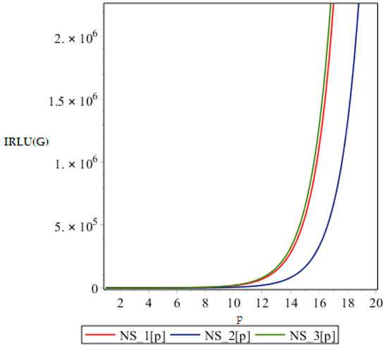
Figure 5.
Graph of .
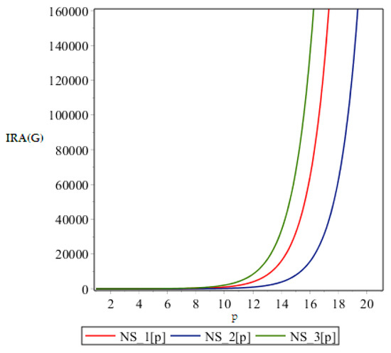
Figure 6.
Graph of .
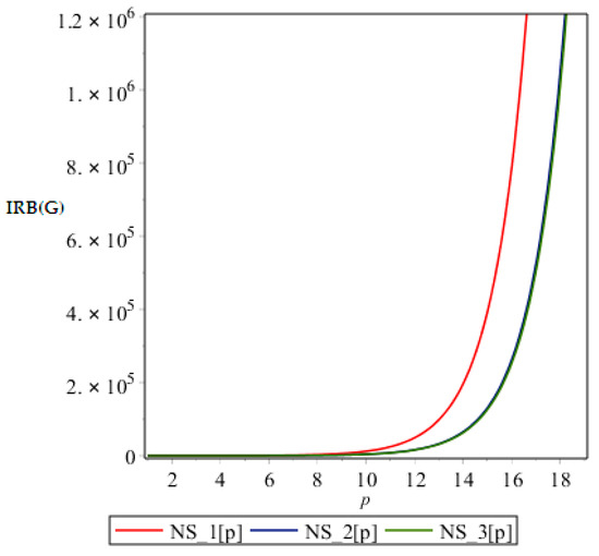
Figure 7.
Graph of .
.
From above graph it seems obvious that irregularities have a slight increase with an increase in the step size p for the range p ≤ 12. But after p ≥ 14, these irregularity indices drastically increase with increase in p. So NS3[p] is the most irregular and asymmetric structure as far as most of the irregularity indices are concerned. Nanostar dendrimers are relatively less irregular, and NS1[p] are the most regular dendrimers. This trend is not restricted to only irregularity index Most of the irregularity indices behave pretty similarly as shown in the following figures. All other figures show the trends which can easily be understood in the Figure 5, Figure 6 and Figure 7.
All above graphs (Figure 4, Figure 5, Figure 6 and Figure 7) indicate that NS3[p] is highly asymmetric as far as all irregularity indices are concerned, whereas NS1[p] is less asymmetric, and NS2[p] is the most regular structure with respect to all indices. In , NS1[p] and NS3[p] show the same irregularity behavior. These facts typically relate geometry and topology of the structure of these dendrimers and can be used in modelling purposes.
We foresee that our results could play an important role in determining properties of these dendrimers such as enthalpy, toxicity, resistance and entropy. Similar research has been done in [29], where authors discussed some properties of alkane isomers.
Author Contributions
Z.H. and M.M. gave the idea; H.A., T.H. and S.R. wrote the article; S.M.K. and Y.C.K. edited and verified the results.
Funding
This work was supported by the Dong-A University research fund.
Acknowledgments
We are greatly thankful to reviewers for their comments which have helped bring this article to its current form.
Conflicts of Interest
Authors declare no conflict of interests.
References
- Hodge, P. Polymer science branches out. Nature 1993, 362, 18–19. [Google Scholar] [CrossRef]
- Fischer, M.; Vögtle, F. Dendrimers: From design to applications—A progress report. Angew. Chem. Int. Ed. 1999, 38, 884–905. [Google Scholar] [CrossRef]
- Wiener, E.C.; Auteri, F.P.; Chen, J.W.; Brechbiel, M.W.; Gansow, O.A.; Schneider, D.S.; Belford, R.L.; Clarkson, R.B.; Lauterbur, P.C. Molecular dynamics of ion-chelate complexes attached to dendrimers. J. Am. Chem. Soc. 1996, 118, 7774–7782. [Google Scholar] [CrossRef]
- Rucker, G.; Rucker, C. On topological indices, boiling points, and cycloalkanes. J. Chem. Inf. Comput. Sci. 1999, 39, 788–802. [Google Scholar] [CrossRef]
- Klavžar, S.; Gutman, I. A Comparison of the Schultz molecular topological index with the Wiener index. J. Chem. Inf. Comput. Sci. 1996, 36, 1001–1003. [Google Scholar] [CrossRef]
- Gutman, I.; Polansky, O.E. Mathematical Concepts in Organic Chemistry; Springer: New York, NY, USA, 1986. [Google Scholar]
- Randic, M. On the characterization of molecular branching. J. Am. Chem. Soc. 1975, 97, 6609–6615. [Google Scholar] [CrossRef]
- Wiener, H. Structural determination of paraffin boiling points. J. Am. Chem. Soc. 1947, 69, 17–20. [Google Scholar] [CrossRef] [PubMed]
- Estrada, E. Atomic bond connectivity and the energetic of branched alkanes. Chem. Phys. Lett. 2008, 463, 422–425. [Google Scholar] [CrossRef]
- Kier, L.; Hall, L. Molecular Connectivity in Chemistry and Drug Research; Academic Press: New York, NY, USA, 1976. [Google Scholar]
- Kier, L.B.; Hall, L.H. Molecular Connectivity in Structure Activity Analysis; Wiley: New York, NY, USA, 1986. [Google Scholar]
- Deng, H.; Yang, J.; Xia, F. A general modeling of some vertex-degree based topological indices in benzenoid systems and phenylenes. Comput. Math. Appl. 2011, 61, 3017–3023. [Google Scholar] [CrossRef]
- Zhang, H.; Zhang, F. The Clar covering polynomial of hexagonal systems. Discret. Appl. Math. 1996, 69, 147–167. [Google Scholar] [CrossRef]
- De, N.; Nayeem, S.M.A. Computing the F-index of nanostar dendrimers. Pac. Sci. A Nat. Sci. Eng. 2016, 18, 14–21. [Google Scholar] [CrossRef][Green Version]
- Siddiqui, M.K.; Imran, M.; Ahmad, A. On Zagreb indices, Zagreb polynomials of some nanostar dendrimers. Appl. Math. Comput. 2016, 280, 132–139. [Google Scholar] [CrossRef]
- Madanshekaf, A.; Ghaneei, M. Computing two topological indices of nanostars dendrimer, Optoelectron. Adv. Mater. Rapid Commun. 2010, 4, 1849–1851. [Google Scholar]
- Madanshekaf, A.; Moradi, M. The first geometric-arithmetic index of some nanostar dendrimers. Iran. J. Math. Chem. 2014, 5, 1–6. [Google Scholar]
- Munir, M.; Nazeer, W.; Rafique, S.; Kang, S.M. M-polynomial and related topological indices of Nanostar dendrimers. Symmetry 2016, 8, 97. [Google Scholar] [CrossRef]
- Munir, M.; Nazeer, W.; Rafique, S.; Nizami, A.R.; Kang, S.M. M-polynomial and degree-based topological indices of Titania nanotubes. Symmetry 2016, 8, 117. [Google Scholar] [CrossRef]
- Munir, M.; Nazeer, W.; Rafique, S.; Kang, S.M. M-Polynomial and Degree-Based Topological Indices of Polyhex Nanotubes. Symmetry 2016, 8, 149. [Google Scholar] [CrossRef]
- Munir, M.; Nazeer, W.; Shahzadi, S.; Kang, S.M. Some invariants of circulant graphs. Symmetry 2016, 8, 134. [Google Scholar] [CrossRef]
- Chartrand, G.; Erdos, P.; Oellermann, O. How to define an irregular graph. Coll. Math. J. 1988, 19, 36–42. [Google Scholar] [CrossRef]
- Majcher, Z.; Michael, J. Highly irregular graphs with extreme numbers of edges. Discret. Math. 1997, 164, 237–242. [Google Scholar] [CrossRef]
- Behzad, M.; Chartrand, G. No graph is perfect. Am. Math. Mon. 1967, 74, 962–963. [Google Scholar] [CrossRef]
- Horoldagva, B.; Buyantogtokh, L.; Dorjsembe, S.; Gutman, I. Maximum size of maximally irregular graphs. MATCH Commun. Math. Comput. Chem. 2016, 76, 81–98. [Google Scholar]
- Liu, F.; Zhang, Z.; Meng, J. The size of maximally irregular graphs and maximally irregular triangle–free graphs. Graphs Comb. 2014, 30, 699–705. [Google Scholar] [CrossRef]
- Collatz, L.; Sinogowitz, U. Spektren endlicher Graphen. In Abhandlungen aus dem Mathematischen Seminar der Universität Hamburg; Springer: Berlin, Germany, 1957; Volume 21, pp. 63–77. [Google Scholar]
- Bell, F.K. A note on the irregularity of graphs. Linear Algebra Appl. 1992, 161, 45–54. [Google Scholar] [CrossRef]
- Albertson, M. The irregularity of a graph. Ars Comb. 1997, 46, 219–225. [Google Scholar]
- Vukičević, D.; Graovac, A. Valence connectivities versus Randić, Zagreb and modified Zagreb index: A linear algorithm to check discriminative properties of indices in acyclic molecular graphs. Croat. Chem. Acta 2004, 77, 501–508. [Google Scholar]
- Abdo, H.; Brandt, S.; Dimitrov, D. The total irregularity of a graph. Discret. Math. Theor. Comput. Sci. 2014, 16, 201–206. [Google Scholar]
- Abdo, H.; Dimitrov, D. The total irregularity of graphs under graph operations. Miskolc Math. Notes 2014, 15, 3–17. [Google Scholar] [CrossRef]
- Abdo, H.; Dimitrov, D. The irregularity of graphs under graph operations. Discuss. Math. Graph Theory 2014, 34, 263–278. [Google Scholar] [CrossRef]
- Gutman, I. Topological Indices and Irregularity Measures. J. Bull. 2018, 8, 469–475. [Google Scholar]
- Reti, T.; Sharfdini, R.; Dregelyi-Kiss, A.; Hagobin, H. Graph irregularity indices used as molecular discriptors in QSPR studies. MATCH Commun. Math. Comput. Chem. 2018, 79, 509–524. [Google Scholar]
- Hu, Y.; Li, X.; Shi, Y.; Xu, T.; Gutman, I. On molecular graphs with smallest and greatest zeroth-Corder general randic index. MATCH Commun. Math. Comput. Chem. 2005, 54, 425–434. [Google Scholar]
- Caporossi, G.; Gutman, I.; Hansen, P.; Pavlovic, L. Graphs with maximum connectivity index. Comput. Biol. Chem. 2003, 27, 85–90. [Google Scholar] [CrossRef]
- Li, X.; Gutman, I. Mathematical aspects of Randic, type molecular structure descriptors. In Mathematical Chemistry Monographs; University of Kragujevac and Faculty of Science: Kragujevac, Serbia, 2006. [Google Scholar]
- Das, K.; Gutman, I. Some properties of the second Zagreb Index. MATCH Commun. Math. Comput. Chem. 2004, 52, 103–112. [Google Scholar]
- Trinajstic, N.N.; Ikolic, S.; Milicevic, A.; Gutman, I. On Zagreb indices. Kemija Industriji 2010, 59, 577–589. [Google Scholar]
- Milicevic, A.; Nikolic, S.; Trinajstic, N. On reformulated Zagreb indices. Mol. Divers. 2004, 8, 393–399. [Google Scholar] [CrossRef] [PubMed]
- Gupta, C.K.; Lokesha, V.; Shwetha, S.B.; Ranjini, P.S. On the symmetric division DEG index of graph. Southeast Asian Bull. Math. 2016, 40, 59–80. [Google Scholar]
- Balaban, A.T. Highly discriminating distance based numerical descriptor. Chem. Phys. Lett. 1982, 89, 399–404. [Google Scholar] [CrossRef]
- Furtula, B.; Graovac, A.; Vukičević, D. Augmented Zagreb index. J. Math. Chem. 2010, 48, 370–380. [Google Scholar] [CrossRef]
- Das, K.C. Atom-bond connectivity index of graphs. Discret. Appl. Math. 2010, 158, 1181–1188. [Google Scholar] [CrossRef]
- Estrada, E.; Torres, L.; Rodríguez, L.; Gutman, I. An atom-bond connectivity index: Modeling the enthalpy of formation of alkanes. Indian J. Chem. 1998, 37A, 849–855. [Google Scholar]
- Iqbal, Z.; Aslam, A.; Ishaq, M.; Aamir, M. Characteristic study of irregularity measures of some Nanotubes. Can. J. Phys. 2019. [Google Scholar] [CrossRef]
- Gao, W.; Aamir, M.; Iqbal, Z.; Ishaq, M.; Aslam, A. On Irregularity Measures of Some Dendrimers Structures. Mathematics 2019, 7, 271. [Google Scholar] [CrossRef]
- Gao, W.; Abdo, H.; Dimitrov, D. On the irregularity of some molecular structures. Can. J. Chem. 2017, 95, 174–183. [Google Scholar]
- Hussain, Z.; Rafique, S.; Munir, M.; Athar, M.; Chaudhary, M.; Ahmad, H.; Min Kang, S. Irregularity Molecular Descriptors of Hourglass, Jagged-Rectangle, and Triangular Benzenoid Systems. Processes 2019, 7, 413. [Google Scholar] [CrossRef]


© 2019 by the authors. Licensee MDPI, Basel, Switzerland. This article is an open access article distributed under the terms and conditions of the Creative Commons Attribution (CC BY) license (http://creativecommons.org/licenses/by/4.0/).