Article

Handling Constraints and Raw Material Variability in Rotomolding through Data-Driven Model Predictive Control

by
Abhinav Garg
,
Hassan A. Abdulhussain
,
Prashant Mhaskar
* and
Michael R. Thompson
Department of Chemical Engineering, McMaster University, Hamilton, ON L8S 4L8, Canada
*
Author to whom correspondence should be addressed.
Processes 2019, 7(9), 610; https://doi.org/10.3390/pr7090610
Submission received: 29 July 2019 / Revised: 3 September 2019 / Accepted: 5 September 2019 / Published: 10 September 2019
(This article belongs to the Special Issue Computational Methods for Polymers)

Abstract

:
This work addresses the problems of uniquely specifying and robustly achieving user-specified product quality in a complex industrial batch process, which has been demonstrated using a lab-scale uni-axial rotational molding process. In particular, a data-driven modeling and control framework is developed that is able to reject raw material variation and achieve product quality which is specified through constraints on quality variables. To this end, a subspace state-space model of the rotational molding process is first identified from historical data generated in the lab. This dynamic model predicts the evolution of the internal mold temperature for a given set of input move trajectory (heater and compressed air profiles). Further, this dynamic model is augmented with a linear least-squares based quality model, which relates its terminal (states) prediction with key quality variables. For the lab-scale process, the chosen quality variables are sinkhole area, ultrasonic spectra amplitude, impact energy and shear viscosity. The complete model is then deployed within a model-based control scheme that facilitates specifying on-spec products via limits on the quality variables. Further, this framework is demonstrated to be capable of rejecting raw material variability to achieve the desired specifications. To replicate raw material variability observed in practice, in this work, the raw material is obtained by blending the matrix resin with a resin of slightly different viscosity at varying weight fractions. Results obtained from experimental studies demonstrate the capability of the proposed model predictive control (MPC) in meeting process specifications and rejecting raw material variability.

Graphical Abstract

1. Introduction

Rotational Molding or rotomolding is a plastics processing batch process used for the manufacture of seamless hollow plastic products [1]. The process consists of distinct heating and cooling phases. The process constitutes filling a mold with powdered charge and rotating it slowly in a heated oven (using heaters) causing the resin to soften and stick to the walls. Continuously rotating the mold during the subsequent cooling phase produces an end product with even wall thickness. The products tend to be quite large including household water tanks and fuel tanks for agricultural equipment and marine vessels, which means that poor control over part quality results in substantial waste costs for a company. The key objectives in rotational molding are to obtain products, from one batch to another, with desired characteristics consistently while avoiding incomplete sintering or degradation due to extended overheating. Minimized wastage requires a quality control framework capable of compensating for lot-to-lot variance in the properties of the initial charge, and determining process ‘recipes’ meeting user-specified bounds on the quality variables, especially in for cases like the rotomolding example where the quality variables are not available for measurement during the process [2].
One approach to achieving the objectives is to develop a first-principles/physics-based model that will predict the evolution of the process variables based on candidate input variables. That model can be used to design a controller to achieve an on-spec product. Realistic incorporation of heat transfer, discrete particle dynamics and polymer rheology for this first-principles approach necessitate a very complex model structure with a high number of parameters. As is often the case, the development of a realistic mechanistic model is a difficult task, and even if developed, might be very challenging to maintain, or to use for optimization and control. Thus the first principles model-based model predictive control (MPC) [3,4,5] implementations remain elusive for rotomolding control.
In the absence of good first principles model, rotational molding processes have utilized recipe-based open loop policy. Thus, input trajectories that could yield a desired product are determined through a large number of experiments for a new product, yielding high waste rates. The assumption here is that by repeating previous successful input profiles, a desired product could be replicated. However, this approach is susceptible to disturbances, and, equally importantly, requires to be entirely redone for a different set of quality attribute requirements.
Another approach used to partially reject disturbances is trajectory tracking [6]. In this approach, a key measured process variable (such as the internal mold temperature), is tracked to a predefined set-point trajectory. However, even perfect trajectory tracking may not yield the desired product quality because of the possible change in the relationship between the measured/tracked variable and final quality variable due to varying process conditions across batches.
An abundance of historical data in most industrial processes has motivated the development of data-driven modeling and batch quality control approaches. Partial least squares (PLS) is one of the most popular and widely used batch process modeling methods. These models capture the essence of the process dynamics in a projected (lower) dimensional space known as latent space [7,8]. colorredThe PLS model structure resembles linear time-varying (LTV) models. These models predict deviations from mean past trajectories and relate to differences in final product quality. The PLS based modeling approach requires the batches to be of the same duration, which is seldom a case in practice. The remedy is to recognize an appropriate alignment variable for the training and validation batches. While this problem can generally be handled in the context of process monitoring, or control of fixed length batches, the use of these techniques for batches where the batch duration itself could be a decision variable, remains challenging.
More recently, data-driven model designs for continuous processes [9,10,11] were adapted and a subspace identification based batch modeling and control approach was proposed [12]. Here, the past batch database is used to determine a linear time-invariant (LTI) state-space model of the batch process. The approach, in order to capture nonlinear process dynamics, draws on utilizing a high number of ‘states’ as required. The merit of this approach lies in its ability to accommodate batches with variable duration without the need for batch alignment, as demonstrated through varied applications [2,12,13,14,15].
In a recent work [2], this approach has been used for rotomolding to achieve desired product quality specifications. The results [2] demonstrate the efficacy of the approach in terms of achieving improved product quality in validation batches, and the capability to achieve a specified product by expressing appropriate weights on the quality variables in the objective function of the resultant MPC optimization and control implementation. In practice, the rotomolding operation often has to grapple with minor yet significant raw material variability, manifested as varying flowability of the input charge from one molded part to another. The other challenge with the former approach [2] of indirectly enforcing quality requirements through the objective function is that a careful design of the objective function is required. The practitioner has to identify the desired batches from historical data and decide on the weights in the objective function such that minimization/maximization of quality variables will result. A much more intuitive, practical and desirable way for the practitioner to specify quality is through placing constraints on the quality variables.
Motivated by these considerations, this work presents a subspace identification based modeling and control approach for handling user-specified quality through constraints and demonstrates explicitly the ability to reject raw material variability in a rotational molding process. For the presented study, the raw material variability observed in practice is replicated in this case by blending the matrix polymer resin with a near-similar resin with slightly different flow properties. The rest of the paper is structured as follows: Section 2 describes the rotomolding process and reviews the batch subspace identification approach. The proposed MPC design is presented in Section 3 and closed-loop experimental results presented in Section 4. Finally, a few concluding remarks are made in Section 5.

2. Preliminaries

In this section, a brief overview of the rotational molding process used in this work and batch subspace identification based process modeling technique is given. This section forms the basis for the proposed novel MPC design and corresponding closed-loop results presented in Section 3 and Section 4 respectively.

2.1. Rotational Molding

In this work, a high density powder (ExxonMobilTM HD 8660.29, Imperial Oil, Sarnia, ON, Canada) and a linear low density polyethylene powder (ExxonMobilTM LL 8460.29, Imperial Oil, Sarnia, ON, Canada) were utilized. Both resins were donated by Imperial Oil Ltd. The melt flow index (MFI) of HD 8660.29 is 2 g/10 min, while the MFI of LL 8460.29 is 3 g/10 min. Both MFI were tested with a standard weight of 2.16 kg according to ASTM Standard D1238-13. The melt temperature of HD 8660.29 and LL 8460.29 are 129 °C and 126 °C respectively, according to the vendor.
The samples were prepared using a laboratory-scale uni-axial rotational molding machine (see Figure 1, McMaster University, Hamilton, ON, Canada) with a custom LabVIEW program (National Instruments Corporation, Austin, TX, USA) for setting the inputs to the system. The input includes power to the left and right panels of the oven heater and the compressed air supply, with the measured variable being the internal air temperature profile inside the mold. The internal temperature was monitored using a K-type thermocouple mounted in the center of the mold, while heater temperature was monitored by similar thermocouples mounted against the respective panels. For every batch, a charge of 100 g of HD 8660.29 (matrix resin) or HD 8660.29 blended with a small fraction of LL 8460.29 was loaded into the mold. The mold was then closed and rotated at a constant speed of 4 RPM (rotations per minute). The oven was heated to 300 ° C and lowered from above to surround the mold. A MATLAB (The Mathworks Inc., Natick, MA, USA) script was run to control the trajectory of the internal air temperature. After the mold reached the optimal number of control steps determined by the proposed approach, the oven was removed and a stream of forced air applied at a speed of 2.5 m/s was used to cool the mold to 80 °C (internal temperature). Thereafter, the sample is taken out of the mold for further characterization. The final dimensions of the mold were a 90 × 90 × 3 mm cube though only the four peripheral walls are coated with polymer during processing. The measurement technique for the quality variables is described in the next section.

2.1.1. Surface Void Analysis

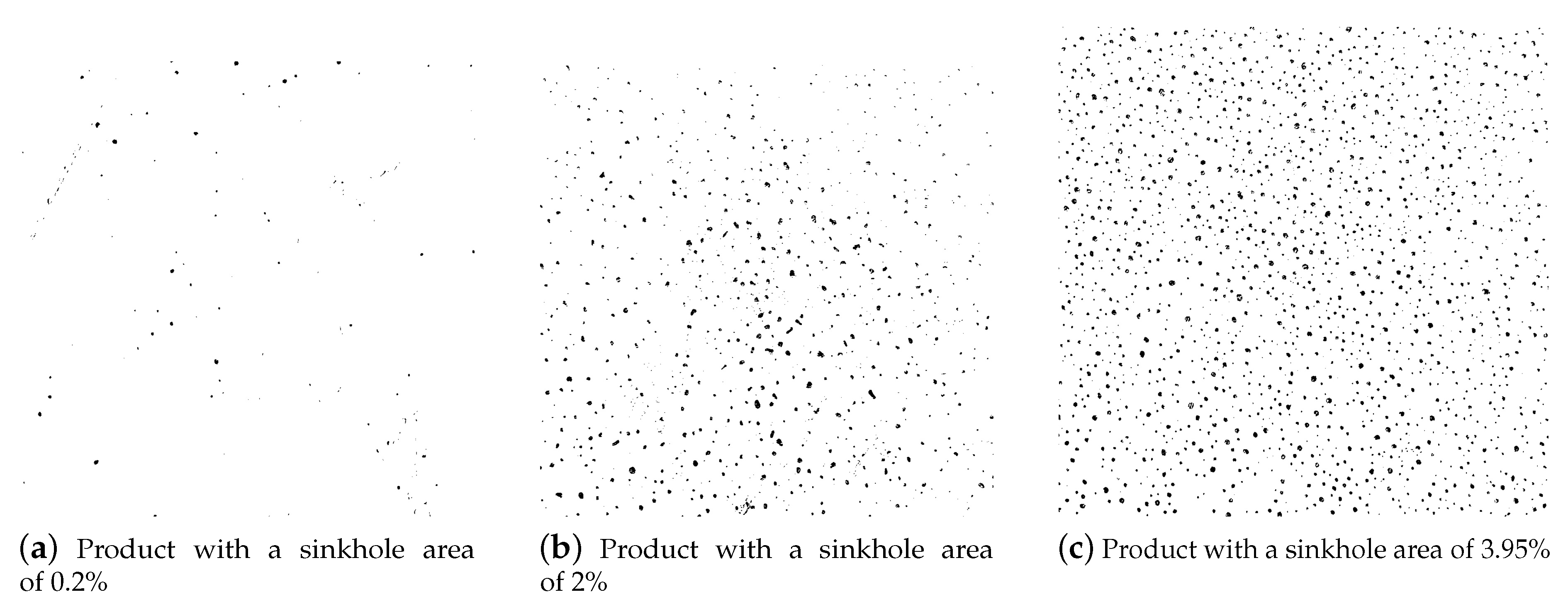
The quality of a molded part is determined based on the completeness by which the polymer particles sinter together during heating. Both the strength and appearance of the part are related to this factor of processing. One measurable quality parameter to assess the completeness of sintering is to visually inspect the molded wall for voids. To highlight the surface voids of an otherwise white-colored sample, a low viscosity lubricant containing a mixture of copper and graphite particles was rubbed onto one of the faces of a sample, with the excess lubricant removed using a paper towel. An image of the face is taken using a digital camera and image analysis software was utilized to estimate the void area for a 40 × 40 mm section. The sinkhole area was calculated by dividing the void area by the area of the section (1600 mm2). Figure 2 shows the processed image of a product with a sinkhole area of 0.2%, 2%, and 3.95%. A good product is often expected to have the smallest void area which suggests completeness of sintering and thus better appearance and impact properties of the product.

2.1.2. Ultrasonic Spectroscopy

While mechanical testing can destructively test the quality of a part for completeness of sintering, new non-destructive methods based on acoustics are gaining acceptance and this study sought to maximize the possibility of data collection related to the rotomolding process. Ultrasonic testing for one of the faces of the uncut sample was carried out using the same setup as reported in previous studies [16]. The acoustic transducers (R15a, resonant and F30, broadband by Physical Acoustics, Physical Acoustics Corporation, Princeton Junction, NJ, USA) were attached to the face of the sample using high vacuum grease (Dow Corning), being kept 55 mm apart. A series of signals were emitted successively between 135 to 165 kHz in 1 kHz steps. Each signal propagated through the sample and was recorded at a rate of 4 MHz using a data acquisition system by National Instruments. The detected signals were converted to the frequency domain using a fast Fourier transform and combined into a single spectrum. This quality variable corresponded to the maximum amplitude (from all 31 signals emitted).

2.1.3. Impact Test

Samples were cut and frozen at −40 °C for 24 h in preparation for dart impact testing. The initial falling dart height was selected at 0 . 762 m ( 2 . 5 ft) and moved using the staircase method based on whether the sample failed from impact at its current height. A standard dart weight of 6 . 804 kg (15 lbs) was utilized for this test. If the sample failed, then the height of the dart is decreased by 0 . 1524 m ( 0 . 5 ft), whereas if the sample did not fail, then the height of dart should be increased by 0 . 1524 m. The impact energy was calculated based on the height where 50 % of the samples failed (each face of the mold being used for analysis from each batch, thus resulting in four measurements, to ultimately yield an average value).

2.1.4. Rheology

As any polymer is heated, it experiences thermal damage. Initially, the harm is minor but as time progresses, the damage can significantly affect physical properties. During rotational molding, this degradation proceeds over the course of molding a part and at a certain period of time, the benefits to complete sintering are offset by the damage to the polymer. Degradation of a Sample was monitored in this study by measuring resin viscosity using a 25 mm parallel plate rheometer (DHR TA Instruments, TA Instruments, New Castle, DE, USA). A frequency sweep test was implemented at a strain of 0 . 15 covering shear rates between 0 . 1 to 200 s−1 for a temperature of 190 °C. Three tests are performed per sample to account for measurement variation. The data was fit using the Cross model as shown in Equation (1) using the TRIOS instruments software (TA Instruments, New Castle, DE, USA):
η = η + η 0 η 1 + ( C γ ˙ ) m
Here, η is shear viscosity, η is the infinite-shear viscosity parameter, η 0 is the zero-shear viscosity parameter, C is the Cross time constant, γ ˙ is the shear rate constant and m is the Cross rate constant. In this work, only the zero-shear viscosity was considered as the representative quality parameter for thermal degradation. Other parameters were not evaluated in the quality model.

2.2. Subspace Identification Approach for Batch Processes

To obtain a desired product quality consistently across batches, a model based control framework is necessary. This requires a good process model capable of predicting the process and quality variable evolution for a candidate input sequence. In our proposed approach, we achieve this by first identifying a dynamic model for predicting the internal mold temperature given a candidate heater power and compressed air flow rate profile. This model is then augmented with another model that captures the relationship between the final quality and the end point state prediction of the dynamic model.
In the present work, a deterministic subspace identification algorithm, adapted for batch processes, is used to identify the dynamic process model. The deterministic identification problem is that of determining the order n and system matrices of a state space model given input and output measurements. The identified model takes the following form:
x k + 1 d = A x k d + B u k ,
y k = C x k d + D u k ,
where A R n × n , B R n × m , C R l × n , D R l × m are the associated system matrices and are determined up to within a similarity transformation.
Subspace identification methods are non-iterative in nature and compute the unknown parameters using matrix algebra (see, e.g., [17,18]) which distinguishes them from classical system identification approach (see, e.g., [19]). A number of algorithms have been proposed in subspace identification among which some of the most prominent ones include canonical variate analysis (CVA) [20], numerical algorithms for subspace state space system identification (N4SID) [21] and multivariable output error state space algorithm (MOESP) [22]. These algorithms differ only in the weighting of the matrix used at the singular value decomposition step as shown in [23]. However, these algorithms were designed primarily for continuous processes (see, e.g., [11,24,25]). Thus, the training datasets are obtained through identification experiments carried around a desired steady-state condition. This facilitates straightforward construction of Hankel matrices within the subspace identification algorithm.
In contrast, in a batch process data is collected from multiple batches with the objective of identifying a model for the transient dynamics of the process. For instance, consider the output measurements of a batch process denoted as y b k , where k is the sampling instant since batch initiation, and b denotes the batch index. The output Hankel matrix for a batch b is given by:
Y 1 | i b = y b 1 y b 2 y b j b y b i y b i + 1 y b i + j b 1
The key question then is how to appropriately utilize data from multiple batches. In essence, the significant difference in the structure of data collected in batch processes, in comparison to continuous processes, calls for specific adaptation of the batch database and subspace identification algorithms. A naive concatenation of the historical batches data into one ‘continuous’ data-set would result in the incorrect assumption that starting point of one batch is similar to the previous batch’s end-point. The solution is to construct a single pseudo-Hankel matrix for both input and output data such that it recognizes the batch nature of the data. This is done by constructing pseudo-Hankel matrices of the following form [12]:
Y 1 | i = Y 1 | i 1 Y 1 | i 2 Y 1 | i n b ,
where, n b is the number of batches used for training. Similarly, pseudo-Hankel matrices for input data are formed. This method does not require batches to be of same duration and thus mean-centring around nominal trajectory or calculation of an alignment variable are not required. This is in contrast to the time-dependent modeling approaches such as PLS.
Past the formation of the pseudo Hankel matrices, the deterministic algorithm presented in [26], and appropriately adapted in [12] is used for modeling of the rotational molding process. Note that in principle, the batch subspace identification algorithm discussed above can be used with appropriately adapting existing subspace identification algorithms. After obtaining the state trajectories, the system matrices are estimated using ordinary least squares (see [27] for detailed discussion of the algorithm).

2.3. Model Identification

The current lab scale rotational molding process consists of three inputs and one output variable. Control action for two heaters and a compressed air supply constitutes the process manipulated inputs while mold internal temperature is the measured output. For the model identification, a database consisting of 10 different batches is used. The database is segregated into training and validation batches, utilizing seven batches for training, while keeping the remaining three for validation purposes. As evidenced by the validation test, the training batches provide a sufficiently rich data set for model identification. The richness is due to the variation in the heating cycle time across batches thereby covering a large enough operating space for the process. A model only for the heating cycle is identified in this work. No control action was active during the cooling phase.
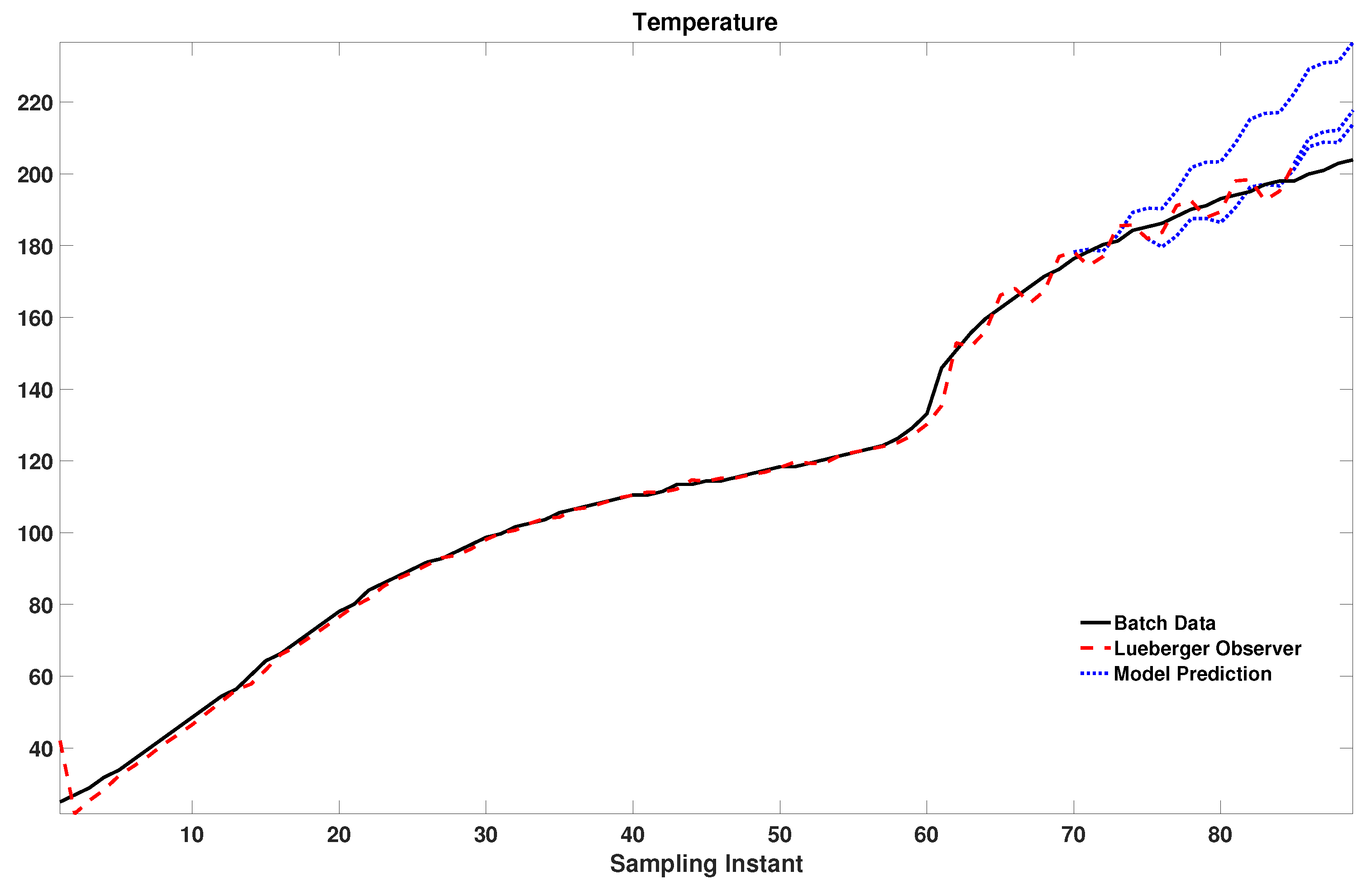
Subsequently, a state-space model of order two was identified using the proposed approach as discussed in Section 2.2. The model order was selected to ensure good prediction of the internal mold temperature in the validation batches. The open-loop model predictions for one of the validation batches was as shown in Figure 3. Model predictions from 70th, 75th and 85th sampling instants are shown. It can be observed from the figure that as the batch progresses, more data becomes available which results in improved model predictions.
The identified state-space model alone is not sufficient to predict the quality of the finished sample at the completion of batch. For this, it is augmented with a least squares based linear quality model obtained by relating the terminal states of the state-space model to the quality measurements of the training batches (see Table 1) as follows.
Q t f = L ^ m x [ t f h e a t ] + e ,
where Q t f denote quality measurements at the termination of batch at time t f , L ^ m is the matrix relating the terminal states to the terminal quality, x [ t f h e a t ] are terminal states of the subspace model (i.e., at completion of the heating cycle at time t f h e a t ) and e represents white noise. The predictions for the validation batch using the identified quality model are as listed in the Table 2. It can be observed that the predictions in general improve as batch progresses and are close to the actual values. In summary, the state space model together with this quality model completely describes the dynamics of the rotomolding process. Note that in this work internal mold temperature prediction alone formed the criterion for order selection of the state space model. An alternative is to incorporate the quality model predictions as well in the decision making.

3. Model Predictive Control Design for Rotational Molding Process

The state space model along with the quality model, as described in the previous section, results in a model capturing the process dynamics sufficiently well. The second step in data-driven modeling and control approach is then to incorporate this data-driven model with an MPC scheme to achieve desired product quality. A primary requirement on the model, for it to be suitable in MPC, is its ability to make reasonable prediction of the process evolution. In our proposed approach, good model predictions are direct function of the initial state estimates and the state-space (and quality) model matrices. As the initial state information for a new batch is not available upfront, the approach requires state estimation during initial operation of the batch. To achieve this, a PI controller is used till the internal mold temperature reached 130 °C, a predefined threshold in this work. During this phase, control actions for the two heaters and the compressed air supply are obtained by set-point tracking of the two oven temperatures (fixed at 300 °C). Subsequently, a state estimator (a Luenberger observer in the present manuscript, see Equation (6)), is run to obtain state estimates. During this phase of the controller design, essentially the mechanism obtains information regarding the phenomena of heating, adhesion and melting of the powder in that particular batch. Once a reasonable state estimate has been obtained (gauged by the accuracy of the estimated output), the controller is switched to MPC which uses the state information to appropriately control the rest of the sintering (heating) phase. A standard Luenberger observer takes the following form:
x ^ [ k + 1 ] = A x ^ [ k ] + B u [ k ] + L ( y [ k ] y ^ [ k ] ) ,
where L is the observer gain and is designed based on the user specified eigenvalues of ( A LC ) . These are chosen to ensure ( A LC ) is stable (within the unit circle). In MATLAB, this can be achieved using the place command.
In batch operations, the control objective and the manner in which the control horizon evolves are very different in comparison to continuous operation. This requires appropriate controller design for batch processes. Further, in rotational molding control, the length of the heating cycle and thus the batch duration is also a decision variable in the MPC controller design.
The control action was computed and implemented every 10 s through the MATLAB-LabView interface. At a sampling instance l, the optimal input trajectory till the end of the batch was obtained through solution of the following optimization problem:
min U f , l f β Q ^ t f [ l f l ]
s . t . U j , m i n u f [ k ] U j , m a x , 0 k l f l
| u f [ 0 ] u [ l 1 ] | δ ,
| u f [ k ] u [ k 1 ] | δ , 1 k l f l
x ^ [ 0 ] = x ^ [ l ]
l f { t s w i t c h + 300 , t s w i t c h + 350 , t s w i t c h + 400 }
Λ Q ^ t f Γ
x ^ [ k + 1 ] = A x ^ [ k ] + B u f [ k ]
y ^ [ k ] = C x ^ [ k ] + D u f [ k ] 0 k l f l
Q ^ t f = L m x ^ [ l f ]
with,
Q ^ = Q ^ 1 Q ^ 2 Q ^ 3 Q ^ 4 T
β = 1 0 0 1 / 1000
Λ = 1 0 0 0 0 0 0 1
Γ = 2 12000
where, U f = [ u f [ 0 ] , u f [ 1 ] , u f [ l f l ] ] is the decision variable consisting of two heaters and the air supply control action for the remainder of the batch, l f denotes the heating cycle termination time. The set of possible termination times, l f is specified in Equation (7f) based on experience. δ = 30 30 30 T is the permitted rate of input change specified in Equation (7c) and (7d), and U j , m i n and U j , m a x are the specified lower and upper bounds on the manipulated variable (Equation (7b)) with U j , m i n and U j , m a x being 0 0 0 T and 100 100 100 T respectively. In addition, t s w i t c h denotes the time (in sec) at which the controller switches to MPC from PI controller. Equation (7e) denotes the Luenberger observer generated state estimate at the l t h instant. Further, Equation (7g) represents the user-specified constraints on the quality variables. Finally, Equation (7j) specifies the quality model which predicts the terminal product quality using the terminal states (of the heating cycle) which in-turn are predicted by the dynamic model as specified in the Equation (7h) and (7i). In Equation (8a), Q ^ 1 , Q ^ 2 , Q ^ 3 and Q ^ 4 refers to the predicted values of the four quality variables namely, sinkhole area coverage (%), average ultrasonic spectra amplitude (dB), impact energy (Kg.m) and zero-shear viscosity (Pa–s) respectively.
The above optimization problem is essentially a mixed integer linear program (MILP) but is instead solved in a brute force fashion as three linear programs using linprog in MATLAB. Thus, exploiting the limited choices provided for the batch duration, the optimization over the time duration is simply carried out by comparing the optimal solution corresponding to each specific duration, and the best solution is implemented. That is, for each of the three candidate batch duration, the optimization problem is solved, and the objective function evaluated subject to constraints. Subsequently the best solution is chosen. In essence, for each possible batch termination time, a constrained quadratic program is solved. In the present application, only three different values of batch duration are evaluated, thus the computational complexity remains fairly low. Note that in principle, higher resolution of the batch end-times could be evaluated, resulting in increased computational complexity. Given the plant-model mismatch, the resultant benefit might not be significant, thus motivating the relatively modest exploration of the optimally over the batch duration. Thus, at each time step, the controller computes a trajectory for the best duration that would yield the on-spec product, and updates this value as more information is received from the process. Further, the optimization problem is solved in a hierarchical fashion to guarantee feasibility. First, the original optimization problem with all the constraints is solved. If the algorithm runs into feasibility issues, the optimization problem is relaxed by removing the constraint on the quality measurements in Equation (7g). This relaxed version is guaranteed to find a feasible solution due to the nature of the problem ensuring an implementable solution. In our experience, the feasibility is always recovered as the process moves to a new point, and more process output information becomes available. To facilitate the implementation of the proposed control approach on the lab scale experimental setup, MATLAB is interfaced with LabView which in-turn interfaces with the sensors and actuators and works as a data acquisition system.

4. Closed-Loop Experimental Results

The proposed rotomolding modeling and control approach is validated through implementation on the lab-scale experimental setup. Closed-loop implementations with two different objectives are carried out. We first illustrate the ability of the controller to deliver an on-spec product, and then evaluate the ability of the controller to handle raw material variability due to the blending of the matrix resin with a similar resin with slightly different viscosity (judged by its melt index).
In the first implementation, the efficacy of the controller was investigated on five new batches. l f in all of these batches were selected as t s w i t c h + 30 by the MPC in the last iteration; however, it selected other batch lengths as well during the course of control. The feedback control algorithm, proposed in this work, achieved excellent quality results while meeting the desired product constraints (see Table 3). The internal mold temperature and input profiles are shown in Figure 4. Note that the constraints imposed on the quality variables are significantly tighter compared to the training case ( Q 1 constrained to be less than 2%—something that is not achieved in any of the training batches, the least Q 1 observed being 3.88%. On the other hand, the control design recognizes that the constraint on Q 4 is significantly larger than that observed in the training batches, and is able to appropriately push the value of Q 4 higher than that observed in the training, while still respecting the constraint, in turn allowing the tight Q 1 constraint to be met. This ability of the controller to meet target specifications is significant; and generally very difficult to achieve in practice (without the use of such a model-based control design). That is, determining the internal temperature profile (leave alone the heater power and compressed air flow) that would ensure that quality constraints are met, is a very challenging problem to address. In contrast, the present modeling and control approach utilizing a combination of a causal dynamic model and quality model is able to deliver on-spec products consistently.
In the second set of batches, the efficacy of the proposed approach to meet user-specified constraints on product quality under raw material variability is evaluated. In this case the constraints were changed to another possible requirement by the practitioners defined by Λ = 1 0 0 0 0 0 1 0 and Γ = 2 5 . The parameter β in this case was changed to β = 1 0 1 0 and l f { t s w i t c h + 400 , t s w i t c h + 450 , t s w i t c h + 500 } . The rest of the MPC problem was identical to the previous case. The product qualities obtained for this case are listed in Table 4. The internal mold temperature and the input profiles for one of the blends are shown in Figure 5. Again, for all the blends, going up to 10% blending, the controller consistently achieves on-spec product. Note that the initial period of state estimation, where the control design ‘learns’, i.e., the estimation of the state of the system is influenced by the dynamics observed in the current batch. This, together with the feedback element, allows the controller to reject the induced raw material variability while achieving the on-spec product.
Remark 1.
In the present application, the focus was on achieving on-spec product as specified by constraints on the quality variables and demonstrate effective rejection of raw material variability. Thus, other considerations, such as smoothness of input moves were not included in the control design. One could include these considerations explicitly in the control design, and implement these either via appropriate constraints on the rate of input change or putting penalties on the rate of change of input variables in the objective function.
Remark 2.
Note that the present results demonstrate the ability to model the complex dynamics with the power to the two heaters and the cooling fan being treated as three separate inputs. In reality, all three inputs result in a unified heating/cooling effect. The success of this approach also suggests that alternatively, at the model identification step, a principle component analysis can be carried out to reduce the three inputs to one effective input (the principle component representing the heating/cooling). Then model identification step can be set up to use that principle component as part of the modeling process and in turn in the MPC controller. In yet another alternative, the two heaters could be reduced to one input, and the cooling input could be kept separate, and finally an MPC can be designed that focuses on achieving the desired product while minimizing resource usage. Thus, the cost of various inputs could be directly accounted for in the control calculation to design an economic MPC to enable production that directly maximizes profit. In this fashion, regional effects such as costs of electricity could be directly accounted for in the control calculations.
Remark 3.
From an industry practitioner’s point of view, it is important to meaningfully visualize the evolution of the process during the operation. It serves two purposes: (a) visualize the performance of the identified process model in the changing process conditions to assess any need for model update (for instance, see [28]), and (b) predict the evolution of product quality during the batch operation to gauge the possibility of achieving the desired product given a resin. If the monitoring approach determines that the given resin simply cannot yield the desired product, then the particular batch may be terminated early to prevent waste of additional resources.
Remark 4.
The modeling approach proposed in this work results in a linear dynamic state space model coupled with a static quality model. The use of this model within an optimization framework results in a convex problem which is easy to solve. When implementing this approach in a commercial setting, the structure of the model will still be same. Therefore, the strategy would directly scale up for commercial use as the computations for control moves will still be tractable.
Remark 5.
In another work [1,29], the authors explored the possibility of using acoustics data, collected by performing ultrasonic tests on the mold, as an alternative to destructive methods for quality assessment. Future work will also focus on integrating more detailed acoustics data with our modeling approach for modeling and control of the product quality.

5. Conclusions

In this work, a data-driven modeling and control framework is developed capable of handling the problems of uniquely specifying and robustly achieving user-specified product quality in an experimental uni-axial rotomolding process. To this end, a subspace state-space model of the process is identified from historical data which predicts the evolution of the internal mold temperature from a given set of input profiles. This dynamic model is further augmented with a static quality model relating its terminal state predictions with key quality variables. The overall model is then deployed within an MPC scheme that enables achieving on-spec products based on the specified limits on the quality variables along with rejecting the raw material variability. The natural raw material variability observed in the industry is replicated in the pilot experimental setup by blending, in various percentages, the matrix resin with a slightly different one. The experimental results corroborate the ability of the proposed control framework to reject raw material variation and achieve desired product quality specified through explicit constraints on quality variables.

Author Contributions

Conceptualization, P.M. and M.R.T.; methodology, A.G. and P.M.; software, A.G.; experiments, H.A.A. and A.G.; writing—original draft preparation, A.G.; writing—review and editing, A.G., P.M., H.A.A. and M.R.T.; supervision, P.M. and M.R.T.

Funding

Financial support from the McMaster Advanced Control Consortium (MACC) and the Natural Sciences and Engineering Research Council of Canada (Collaborative Research and Development Grant) is gratefully acknowledged.

Acknowledgments

Authors thank Imperial Oil and Ron Cooke for the donation of polyethylene and technical advice on rotomolding process.

Conflicts of Interest

The authors declare no conflict of interest. The funders had no role in the design of the study; in the collection, analyses, or interpretation of data; in the writing of the manuscript, or in the decision to publish the results.

References

  1. Gomes, F.P.; Garg, A.; Mhaskar, P.; Thompson, M.R. Quality Monitoring of Rotational Molded Parts Using a Nondestructive Technique. In Proceedings of the ANTEC 2018, Orlando, FL, USA, 7–10 May 2018; Society of Plastics Engineers: Brookfield, CT, USA, 2018. ISBN 123-0-1234567-8-9. [Google Scholar]
  2. Garg, A.; Gomes, F.P.; Mhaskar, P.; Thompson, M.R. Model predictive control of uni-axial rotational molding process. Comput. Chem. Eng. 2019, 121, 306–316. [Google Scholar] [CrossRef]
  3. Bonvin, D. Optimal operation of batch reactors—A personal view. J. Process Control 1998, 8, 355–368. [Google Scholar] [CrossRef]
  4. Aumi, S.; Mhaskar, P. Integrating Data-Based Modeling and Nonlinear Control Tools For Batch Process Control. AIChE J. 2012, 58, 2105–2119. [Google Scholar] [CrossRef]
  5. Aumi, S.; Corbett, B.; Mhaskar, P.; Clarke-Pringle, T. Data-based modeling and control of Nylon-6, 6 batch polymerization. IEEE Trans. Control Syst. Technol. 2013, 21, 94–106. [Google Scholar] [CrossRef]
  6. Abu-Al-Nadi, D.I.; Abu-Fara, D.I.; Rawabdeh, I.; Crawford, R.J. Control of rotational molding using adaptive fuzzy systems. Adv. Polym. Technol. 2005, 24, 266–277. [Google Scholar] [CrossRef]
  7. Flores-Cerrillo, J.; MacGregor, J.F. Control of particle size distributions in emulsion semibatch polymerization using mid-course correction policies. Ind. Eng. Chem. Res. 2002, 41, 1805–1814. [Google Scholar] [CrossRef]
  8. Flores-Cerrillo, J.; MacGregor, J.F. Latent variable MPC for trajectory tracking in batch processes. J. Process Control 2005, 15, 651–663. [Google Scholar] [CrossRef]
  9. Ljung, L. System Identification: Theory for the User; Pearson Education: London, UK, 1998. [Google Scholar]
  10. Kadali, R.; Huang, B.; Rossiter, A. A data driven subspace approach to predictive controller design. Control Eng. Pract. 2003, 11, 261–278. [Google Scholar] [CrossRef]
  11. Pour, N.D.; Huang, B.; Shah, S.L. Subspace Approach to Identification of Step-Response Model from Closed-Loop Data. Ind. Eng. Chem. Res. 2010, 49, 8558–8567. [Google Scholar] [CrossRef]
  12. Corbett, B.; Mhaskar, P. Subspace identification for data-driven modeling and quality control of batch processes. AIChE J. 2016, 62, 1581–1601. [Google Scholar] [CrossRef]
  13. Garg, A.; Corbett, B.; Mhaskar, P.; Hu, G.; Flores-Cerrillo, J. Subspace-based model identification of a hydrogen plant startup dynamics. Comput. Chem. Eng. 2017, 106, 183–190. [Google Scholar] [CrossRef]
  14. Garg, A.; Mhaskar, P. Subspace Identification-Based Modeling and Control of Batch Particulate Processes. Ind. Eng. Chem. Res. 2017, 56, 7491–7502. [Google Scholar] [CrossRef]
  15. Garg, A.; Mhaskar, P. Utilizing big data for batch process modeling and control. Comput. Chem. Eng. 2018, 119, 228–236. [Google Scholar] [CrossRef]
  16. Gomes, F.P.; West, W.T.; Thompson, M.R. Effects of annealing and swelling to initial plastic deformation of polyethylene probed by nonlinear ultrasonic guided waves. Polymer 2017, 131, 160–168. [Google Scholar] [CrossRef]
  17. Tangirala, A.K. Principles of System Identification: Theory and Practice; Taylor & Francis: Abingdon, UK, 2014. [Google Scholar]
  18. Qin, S.J. An overview of subspace identification. Comput. Chem. Eng. 2006, 30, 1502–1513. [Google Scholar] [CrossRef]
  19. Raghavan, H.; Tangirala, A.K.; Bhushan Gopaluni, R.; Shah, S.L. Identification of chemical processes with irregular output sampling. Control Eng. Pract. 2006, 14, 467–480. [Google Scholar] [CrossRef]
  20. Larimore, W. Canonical variate analysis in identification, filtering, and adaptive control. In Proceedings of the 29th IEEE Conference on Decision and Control, Honolulu, HI, USA, 5–7 December 1990; Volume 2, pp. 596–604. [Google Scholar] [CrossRef]
  21. Overschee, P.V.; Moor, B.D. Two subspace algorithms for the identification of combined deterministic-stochastic systems. In Proceedings of the 31st IEEE Conference on Decision and Control, Tucson, AZ, USA, 16–18 December 1992; Volume 311, pp. 75–93. [Google Scholar] [CrossRef]
  22. Verhagen, M.; Dewilde, P. Subspace model identification Part 1. The output-error state-space model identification class of algorithms. Int. J. Control 1992, 56, 1187–1210. [Google Scholar] [CrossRef]
  23. Van Overschee, P.; De Moor, B. A unifying theorem for three subspace system identification algorithms. Automatica 1995, 31, 1853–1864. [Google Scholar] [CrossRef]
  24. Wang, J.; Qin, S.J. A new subspace identification approach based on principal component analysis. J. Process Control 2002, 12, 841–855. [Google Scholar] [CrossRef]
  25. Qin, S.J.; Lin, W.; Ljung, L. A novel subspace identification approach with enforced causal models. Automatica 2005, 41, 2043–2053. [Google Scholar] [CrossRef] [Green Version]
  26. Moonen, M.; De Moor, B.; Vandenberghe, L.; Vandewalle, J. On- And Off-Line Identification Of Linear State Space Models. Int. J. Control 1989, 49, 219–232. [Google Scholar] [CrossRef]
  27. Mhaskar, P.; Garg, A.; Corbett, B. Modeling and Control of Batch Processes; Advances in Industrial Control; Springer International Publishing: Cham, Switzerland, 2019. [Google Scholar] [CrossRef]
  28. Kheradmandi, M.; Mhaskar, P. Adaptive Model Predictive Batch Process Monitoring and Control. Ind. Eng. Chem. Res. 2018, 57, 14628–14636. [Google Scholar] [CrossRef]
  29. Gomes, F.P.; Garg, A.; Mhaskar, P.; Thompson, M.R. Data-Driven Advances in Manufacturing for Batch Polymer Processing Using Multivariate Nondestructive Monitoring. Ind. Eng. Chem. Res. 2019. [Google Scholar] [CrossRef]
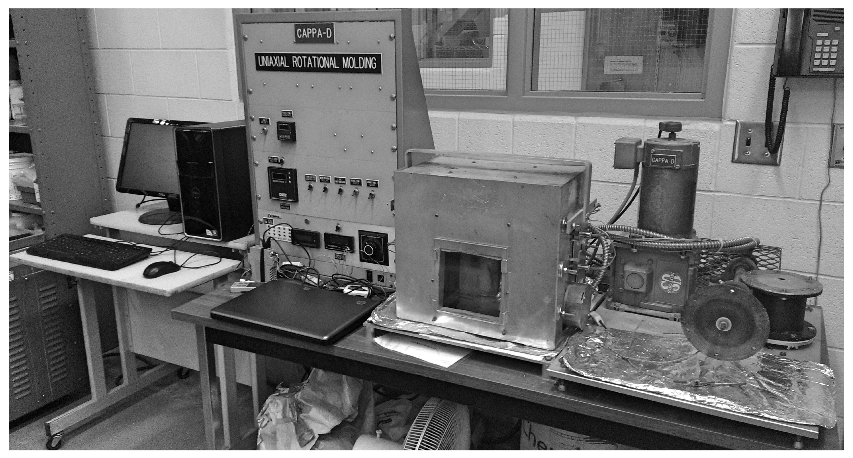
Figure 1. Experimental setup for the rotational molding.
Processes 07 00610 g001
Figure 2. Surface void analysis.
Processes 07 00610 g002
Figure 3. Model validation on a ‘new’ batch (heating phase only).
Processes 07 00610 g003
Figure 4. Zero-blend constrained case.
Processes 07 00610 g004
Figure 5. Varying blends constrained case.
Processes 07 00610 g005
Table 1. Quality measurements for training batches.
Batches Q 1 Q 2 Q 3 Q 4
Batch 1 4 . 42 19 . 27 5 . 70 3596
Batch 2 5 . 46 5 . 43 5 . 18 4260
Batch 3 4 . 15 4 . 90 5 . 70 4276
Batch 4 5 . 41 4 . 59 5 . 70 4230
Batch 5 4 . 30 4 . 15 4 . 67 4441
Batch 6 3 . 88 4 . 31 4 . 15 4377
Batch 7 4 . 78 4 . 65 4 . 67 4387
Table 2. Quality measurements predictions for validation batch.
Batches Q 1 Q 2 Q 3 Q 4
Actual 1 . 45 17 . 30 5 . 18 4681
Predicted ( t = 70 ) 4 . 5 16 . 3 6 . 10 4740
Predicted ( t = 75 ) 4 . 1 14 . 5 5 . 5 4296
Predicted ( t = 85 ) 4 . 1 15 . 3 5 . 5 4292
Table 3. Zero-blend constrained case.
Batches Q 1 2 % Q 2 Q 3 Q 4 12 , 000 P a s
MPC Batch 1 1 . 45 17 . 30 5 . 18 4681
MPC Batch 2 2 . 00 20 . 30 4 . 67 7730
MPC Batch 3 0 . 25 14 . 03 6 . 22 4722
MPC Batch 4 1 . 80 18 . 80 5 . 18 4726
MPC Batch 5 1 . 48 25 . 20 4 . 67 5262
Table 4. Constrained case with varying blends.
BatchesBlending % Q 1 2 % Q 2 Q 3 5   Kg · m
MPC Batch 12 0 . 15 27 . 63 6 . 22
MPC Batch 22 0 . 11 29 . 07 5 . 70
MPC Batch 34 0 . 11 25 . 90 5 . 70
MPC Batch 44 0 . 06 26 . 12 5 . 70
MPC Batch 56 0 . 15 27 . 89 5 . 70
MPC Batch 66 0 . 09 27 . 48 5 . 70
MPC Batch 78 0 . 11 25 . 93 5 . 70
MPC Batch 88 0 . 17 27 . 16 5 . 18
MPC Batch 910 0 . 12 27 . 56 5 . 18
MPC Batch 1010 0 . 18 26 . 93 5 . 70