4.1. The Monitroing Performance of Fluorochemical Engineering Processes
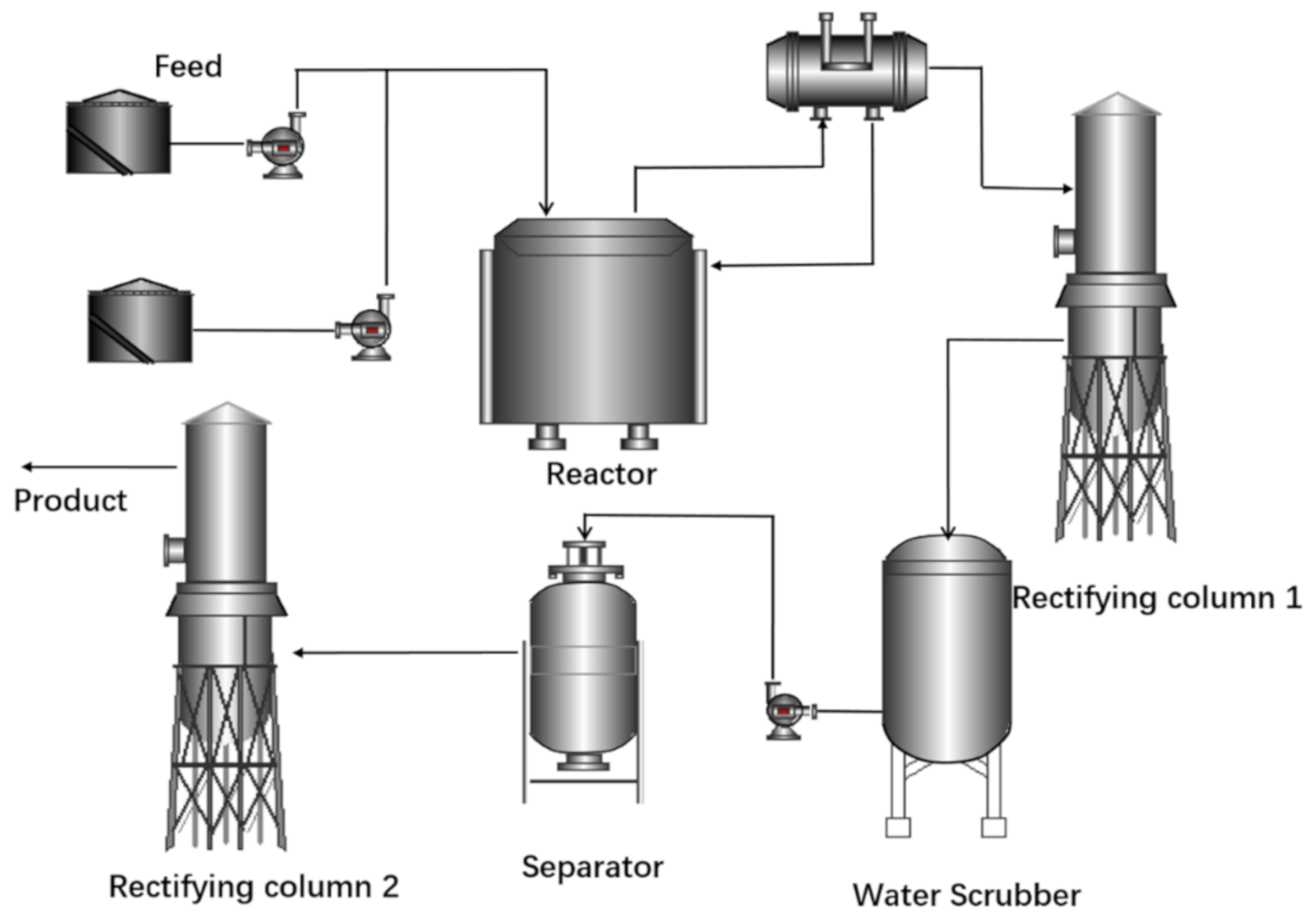
In order to test the effectiveness of the WCNN based multi-model dynamic monitoring method, it was applied to monitoring the R-22 producing process. All data were collected from a fluorination plant located in East China.
Due to the confidentiality agreement, data from only the reaction R-301, which has the biggest impact on the entire production process, and the relevant process were used. The variables are listed in
Table 1. All data were sampled with the sampling interval of 1 min from May to November 2019.
The data of the normal case and five abnormal cases (because they were not serious enough to cause any damage) were selected to verify our WCNN multi-model method. For each case, 8000 samples were used to train the model while 2000 samples were used to test it.
Among these five types of abnormal case, abnormal case 1, 2 and 3 were hard to diagnose even using the regular CNN model. The two-dimensional clustering results of K-means shown in
Figure 5I partly showed how badly they were mixed up with each other. Therefore, they were labeled as HTD cases.
As mentioned in
Section 3.2, the DB wavelet family should be adopted according to the time-varying characteristics of fluoride industrial data signals. It provides compact support and regularity, which means that it has good local performance and can obtain good smoothing effect in signal or image reconstruction [
41]. The ordinal number of the DB wavelet family represents its vanishing moment, which should be selected according to the signal to be processed. Basically, a large order of vanishing moment of a DB wavelet can focus on lower frequency to avoid a high-frequency interference [
42]. With the consideration for the large-scale time-varying characteristics of HTD cases in a fluorine chemical process, DB3 should be selected as the mother wavelet to highlight the low frequency time-varying characteristics without too much detail information lost.
For both preliminary and secondary CNN models, the input size of one sample matrix was 50 × 10, where “50” represented the length of the time series and “10” represented the number of variables. The relevant parameters of both CNN models were described in
Section 3.
The major difficulty in designing a convolutional neural network is that there are no guidelines. We have repeatedly tested and optimized the network structures based on research by Hao and Zhao [
29].
Table 2 shows the diagnostic accuracy of various structures of the secondary CNN model. The performance was measured by fault diagnosis rate (FDR) as:
where
p and
q are the number of faults which are diagnosed correctly and incorrectly, respectively [
43].
The fifth model was selected as the final secondary CNN model. The structure of the preliminary CNN was optimized as: Conv(64)-Pool-Conv(128)-Pool-FC(1024)-FC(4). It can be seen that compared with the preliminary CNN model, the secondary CNN model had two more convolution layers and two more pooling layers. The reason for a simpler structure of the preliminary CNN was to save training or updating time in order to detect all faults as soon as possible. But the secondary CNN structure was much more complex than the preliminary one in order to achieve the purpose of accurately diagnosing HTDs.
The kernel and the pooling layers in both CNN models were optimized to 1 × 2 and 2 × 1, respectively. This design can highlight the correlation among different variables and extract the feature information contained in the time series to the greatest extent considering the computational burden. The “padding” parameter of the convolution layer was set to “SAME” to avoid the adverse effect on feature extraction caused by the limitation of convolution kernel size in considering the corner information. Maximum pooling was utilized to obtain the most important features. The “dropout” was set to 0.5 to avoid overfitting.
The features learned by convolutional neural networks are often high-dimensional, which is difficult to observe and understand intuitively. For example, the array size is 13 × 10 × 128 in our study. In order to visualize the classification results, t-distributed stochastic neighbor embedding (t-SNE) [
44] was used to map the high-dimensional feature output of the convolutional neural network to a two-dimensional space to visualizing the effect of the convolution process. Visualization results of t-SNE is shown in
Figure 5II,III. The digital numbers 0, 1, 2, …, 5 represent samples in normal case and abnormal cases 1 to 5, respectively.
From
Figure 5II, we can see that all samples were badly mixed up. The samples of abnormal cases 4, 5 (two ETDs) and normal case, were distinguished well by the preliminary CNN model. But the samples of HTD cases were partially overlapped in the feature space. After being preprocessed by DWT, as what
Figure 5III shows, they were completely distinguished by the secondary CNN model.
To comprehensively verify the monitoring performance of our prosed method, the monitoring results of these abnormal cases obtained by optimized SVM [
45], DBN [
46] and the traditional CNN [
29] are listed in
Table 3. All models were trained and tested on a computer (Windows 10, I7-4980HQ CPU, RAM 16G).
SVM is a shallow learning method. It was not appropriate to include SVM in this deep-learning application study. But since SVM is a widely used non-linear method, it was used as a reference in our study to demonstrate the improvement the deep learning methods made in FDD. Without any surprise, for ETDs, all methods can detect and diagnose them with 100% FDR. But for HTDs, especially for abnormal case 1, the FDR of SVM was only 65%, which was the lowest. By contrast, the FDR of our WCNN was the best at 90%. For the rest two HTDs diagnosis, it could be seen that even traditional CNN, as a deep learning method, was still not very effective. In contrast, WCNN got the highest FDR (100% and 90%), which mainly due to its unique multi-model strategy and the filtering of redundant information through DWT. The average FDR of WCNN was the highest also, 4.2% higher than the traditional CNN and 6.7% higher than SVM and DBN.
Table 4 shows the difference in average time complexity between traditional CNN and WCNN (the whole procedure was repeated five times). To deal with all the faults including ETDs and HTDs, the traditional CNN not only took a longer time for each single epoch, but also had poorer convergence performance. For WCNN, the preliminary model was easier to converge and only needed 30 epochs. The secondary model was targeted to diagnose only HTDs, whose single epoch needed less training time because of the smaller size of data.
The total training time for our multi-model method was 349 s including 53 s for the preliminary model, 120 s for WT and 176 s for the secondary model. All detection and diagnosis information can be available after 349 s, which is 28 s faster than the traditional CNN method. Considering both the consumed time and the performance, we can see that WCNN obtained 6.7% higher FDR with 28 s faster than the traditional CNN method. It was indeed a comparatively large improvement. More importantly, the training time for the preliminary model was only 53 s, while the training time of the traditional CNN was 377 s. The preliminary model in our multi-model framework still can detect HTD faults even though it could not diagnosis them. It means that it only took 53 s to detect all abnormal status and even to diagnose 40% of them. However, with the traditional CNN, after 377 s the abnormal status can be detected and diagnosed.
Apart from the time consumed by model training as discussed above, inference time is another important criterion. Frames per second (FPS), representing the number of inferences made in a second, is used to define inference speed. Bigger FPS means a faster inference speed of a method. In 10 trials, the inference FPS of the traditional CNN was 30.2. The total FPS of WCNN including the preliminary and the secondary models was 31.8 which were slightly better than that of the traditional CNN. However, the FPS of the preliminary CNN model was 49.3, which means that WCNN can detect an abnormal case 1.6 times faster than traditional CNN. Additionally, the FPS of the secondary CNN model was 90.9, which was three times faster than the traditional one.
For a real industrial process, it is undeniable that we cannot only consider the time of model-making inference. In the R-22 process, the sampling interval is 1 min. In order to meet the requirements of single input matrix, the traditional CNN needs to collect data within 1 h before inputting it for diagnosing. However, WCNN can output the inferential result within 1 min due to its queued updating method, whose details can be found in
Section 3.3. In this instance, the unique method of queue updating in WCNN made a great improvement. The effect of this method was verified by abnormal case 4. WCNN can diagnose and trigger an alarm after 37.2 min and update new results within 1 min. It greatly reduced the time delay in FDD compared with the 60 min of the traditional CNN.
4.2. The Monitoring Performance for the Tennessee Eastman Process
To further verify the generalization performance of our method, it was applied to monitor the Tennessee Eastman (TE) process, a widely used simulation benchmark. The TE process, as a simulation program for real chemical processes, can provide massive amounts of simulated industrial data for advanced process control studies.
Figure 6 illustrates the diagram of the TE process. It contains five major units: a reactor, a stripper, a condenser, a recycle compressor and a separator. A detailed process description including the process variables and the specific plant-wide closed-loop system can be found in the research of Bathelt et al. [
47].
The simulator used in our study is based on the revised version which is available online [
48]. The variables include 12 process-manipulated variables, 22 continuous process measurements and 19 component analysis measurements. Even though there are 28 process fault types in the revised version, IDV1-IDV20 (vector of disturbance flags) in mode 3 (listed in
Table 5) were used in the research of Hao and Zhao [
29]. Therefore, they were also used by us for a fair comparison with the published results using similar algorithms.
Because two variables in mode 3 of the TE process are constants, only the remaining 51 variables were used for monitoring. The sampling period was set to 50 samples/hr. Each sample matrix contained data sampled in one hour, therefore, the matrix size was 50 × 51. The data were collected as follows:
To cover the normal data distribution as comprehensive as possible, the simulator ran in a normal state 10 times with 10 different set points, respectively. For each normal state run, the simulator continued to run for 50 h to collect the normal data for each normal state. Therefore, 25,000 (50 h × 50 samples × 10 times) normal samples were collected in total.
For each IDV state, except for IDV6, the disturbance was introduced after 10 h of normal operation. Then the simulator kept running for another 40 h to collect the IDV data. This simulation process was repeated for 10 times with different production set points. Therefore, 20,000 (40 h × 50 samples × 10times) samples for each IDV were collected.
Because the simulator automatically shut down about 6h after IDV6 was introduced. Only 3000 (6 h × 50 samples × 10 times) samples were collected for it.
The total number of IDV samples was 383,000 and of normal samples was 25,000. Eighty percent of them were used to train the model while the other 20% were used to test it. IDV3, IDV9, IDV15 and IDV16 were considered as HTD IDVs in this paper, because they were hard to diagnose even using deep-learning methods according to the results of published work [
29,
43,
46].
Because there were 17 types of ETD IDV that needed to be diagnosed, the structure of the preliminary CNN was correspondingly complicated. The structures of both the preliminary CNN and the secondary CNN were (Conv (32)-Conv(64)-Pool-Conv(128)-Conv(128)-Pool-FC(1024)-FC (17 or 4)). The “Padding” parameter of the first two convolution layers were set as “VALID”, and the latter were set as “SAME”. Additionally, db5 was selected as the mother wavelet according to the monitoring performance.
In order to verify the performance of this method, diagnosis results were compared with the best results applied to the TE process obtained by other deep-learning algorithms like DBN and the traditional CNN, which were reported by Hao and Zhao and Zhang and Zhao [
29,
46]. The results are listed in
Table 6.
For IDV5, IDV12 and IDV 18, only DBN obtained FDRs for IDV5 and IDV12 testing samples lower than 90%. All other deep-learning methods can diagnose them correctly;
Even IDV3 was considered as one of HTD IDVs, but the performance of all deep-learning methods were all higher than 90%;
For IDV9, a HTD IDV, the test performance for neither DBN nor the regular CNN were good enough. But for WCNN, it was improved to 70%;
For IDV15, another HTD IDV, neither DBN nor the regular CNN could diagnose it. The train performance of WCNN was as high as 98%, but the test performance was only 63%.
For IDV16, the forth HTD IDV, neither DBN nor the regular CNN could diagnose it. However, both training and testing performance of WCNN were good enough (99% and 81%, respectively).
The best average FDR in both training and testing samples obtained by WCNN were the highest ones, which strongly proved its superiority in monitoring.
Using IDV4 as an example, with the queue assembly updating method, the alarm of a fault detection was triggered at the 27.6 min for the first time and was stable after 46.8 min, which was much faster than the 60 min of the traditional CNN.

 ,
, 


