Abstract
The numerical calculation method is used to analyze the wear of the liner of the general structure of a semi-autogenous mill in the axial direction, and the non-uniform wear of each area of the liner is studied to explore the reasons for said wear. The liner is divided into areas along the axial direction, and the discrete element method (DEM) is used to analyze the relationship between the wear volume of each area and the total mass of particles. The composition ratio of the rocks and steel balls in each area, and its relationship with time, are also studied. The results show that the total mass of the particles in the area has a significant effect on the wear of the liner. When the particles are affected by the conical end cover on both sides during the operation of the mill, they will be stratified along the axial direction. The particles with large masses will accumulate on both sides of the mill, and the particles with small masses will be concentrated in the middle of the mill. As a result, the difference between the density and impact energy of rocks and steel balls in each area is caused, and eventually, the mill liner appears to have non-uniform wear.
1. Introduction
A semi-autogenous (SAG) mill is a kind of grinding equipment with crushing and grinding functions. Since it came into being, it has become a favorite in the mineral industry, with its simple process and operation and efficient workability [1]. At the same time, with the success of domestic large-scale SAG mills, especially with the wide application of the SABC (Semi-autogenous ball mill crusher) process, concentrators across the country have begun to use large-scale SAG mills [2,3]. However, while the working method of the SAG mills brings convenience to the beneficiation process, it also brings great constraints. The reduced work efficiency caused by the wear and deformation of the liner, and the system shutdown caused by the replacement of the liner, greatly affect production efficiency. According to the statistics of the Iranian Sar Cheshameh concentrator, the replacement time of the liner accounts for 13% of the entire downtime [4,5]. The non-uniform wear problem of the liners of SAG mills that this research focuses on is also one of the key factors affecting the comprehensive life of the liner. On one hand, the replacement cycle of the liner is determined by overall wear and deformation, and on the other hand, it is also determined by the thinnest part of the worn liner. Therefore, if the wear of the liner can be evened, it can achieve a comprehensive extension of the liner life for the purpose of further improving the working efficiency of SAG mills.
There are many studies on liner wear, and some scholars have paid attention to the problem of non-uniform wear of the liner. The most prominent experimental method is from Iran’s M. Yahyaei, which measures the wear of the liner in the axial direction through a simulation machine and field tests to deduce the wear calculation formula [6,7]. In the follow-up research, through the equal life design method, the non-equal height liner was designed for the non-uniform wear amount of various parts of the area, which alleviated the problem of non-uniform wear of the liner [8]. In terms of numerical simulation, the discrete element method (DEM) is currently the most commonly used numerical calculation method for simulating particle motion states [9]. P.W. Cleary [10] is a pioneer in the study of the mineral industry using DEM. M.S. Powell et al. qualitatively analyzed the changes in the shape of the ball mill liner over working time through the DEM [11]. P.W. Cleary et al. explored the axial movement of rocks and media in a dry ball mill based on the DEM [12]. Xu Lei used the DEM method to predict the wear and impact of each part of the liner’s lifter bar [13]. Zhen Xu used the DEM-FEM (Finite Element Method) coupling method to study the wear of the liner of the ball mill and analyzed the wear of four different surface liners [14]. This kind of multiple simulation method was proposed long ago, the purpose being to make the simulation results closer to reality, but most of the research did not refine the particle size [15].
Although some scholars have paid attention to the problem of liner wear, the research on the liner wear of large-scale SAG mills mostly focuses on the analysis of particle collision energy and contact energy [16]. However, the related research on the causes of this phenomenon of non-uniform wear of the liner is relatively lacking. This research mainly uses the DEM to analyze the mechanism of non-uniform wear of the liner of large-scale SAG mills and provides a theoretical basis for the design of the liner structure to optimize non-uniform wear in the future and further realize the improvement of the work efficiency of large-scale SAG mills.
2. The Current Wear of the Cylinder Liner Structure
The data of this research comes from the SAG mill (8.53 m × 3.96 m) used in the SABC grinding process of a concentrator in Anhui, China. This SAG mill adopts two L-shaped high and low liners arranged back to back, as shown in Figure 1.
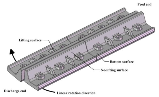
Figure 1.
Arrangement model of the cylinder liner.
The worn liner is shown in Figure 2 is from after about 100 days of work. The lug structure and the boss for protecting the bolts on the liner have been completely worn away, and the bottom of the liner is very thin, but the sides are relatively good. The maximum wear position of the liner at the feed end is 1150 mm from the end, and the maximum wear position of the liner at the discharge end is 500 mm from the end. It is worth noting that the wear of the liner at the discharge end is more serious. Although the wear conditions of the 56 liners on the circle of the cylinder were different, the maximum wear area appeared roughly in the same position, and some liners would even wear through. As shown in Figure 3, to facilitate analysis, the two liners at the feed end and the discharge end were divided into 10 areas in the axial direction. The maximum wear position of the liner at the feed end was between Areas 4 and 5, and the thickness after wear was about 3 mm. The maximum wear position of the liner at the discharge end was in Areas 8 and 9, and the thickness after wear was about 1 mm, at which point it may have even been worn out. The red dot in the figure indicates the position. The red curve on the figure indicates the final thickness of each area in the axial direction of the bottom surface of the liner.
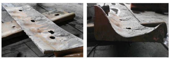
Figure 2.
Worn liner.
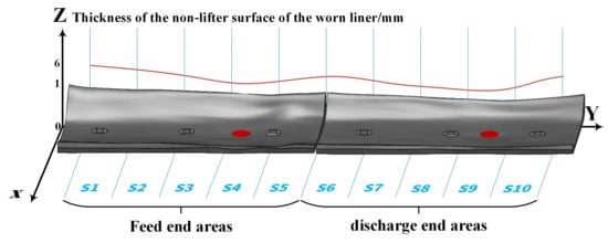
Figure 3.
Schematic diagram of the liner area division and thickness of the bottom surface.
3. Numerical Method
3.1. Research Object
This study uses the EDEM discrete element method simulation software. Due to the difference in models of the SAG mills used in the concentrator, most of the liner structures and layouts were slightly different, but the overall structure and operating principles were similar. Therefore, the results of this study have a generalized reference value in theory and practice. The simulation model parameters were sampled from the aforementioned large-scale SAG mill. The model included liners and two conical end covers for feeding and discharging. The working speed of the SAG mill was 10.6 rpm, it had a total of 56 liners, the height of the lifter bar was 190 mm, both the leading face angle and trailing face angle were 28°, and the height of the small lifter bar was 30 mm, as shown in Figure 4.
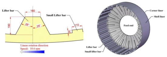
Figure 4.
Cylinder model for simulation.
3.2. Parameter Setting
To make the simulation more realistic in this simulation experiment, the liner material, which included the feed end liner, the discharge end liner, and the shell liner, was consistent with the material used in the concentrator, all of which were chromium-molybdenum steel. The unavoidable wear error value of the steel ball in the operation of the SAG mill was also taken into consideration. The steel ball particle size was set to five different kinds: 150, 130, 110, 90, and 70 mm. The rock was set to a multi-spherical combination shape according to the data of the feed end, including 200, 180, and 60 mm measurements. At the same time, to improve the calculation accuracy of the simulation, the cylinder model would be meshed with ICEM CFD and imported into EDEM. The calculation of the wear used the Hertz–Mindlin model with the Archard wear model, proposed by Professor J.F. Archard. It is believed that the surface wear volume of the model is directly proportional to the work done by the material on the surface and inversely proportional to the surface hardness. The validity of this conclusion has been verified in practice [17]. With the support of this valid conclusion, the parameters used in the simulation model were set as illustrated in Table 1. The wear constant of the model Kc/H = 4.5 × 10⁻¹¹. The coefficient of sliding friction and coefficient of restitution between materials refer to the results of the field test and simulation. At the same time, the setting parameters of other researchers were also taken into consideration [18,19,20]. The simulation parameter setting not only had strong theoretical support, but also passed the industrial verification test. The test result was consistent with the actual working condition, so the data result obtained under this parameter setting had high accuracy and credibility. In this simulation experiment, each simulation ran for 60 s, and the fifth lap was taken as a steady state, so the data results started to count after the fifth lap.

Table 1.
Parameters of a semi-autogenous (SAG) mill liner’s wear in the simulation.
4. Results and Discussion
4.1. The Relationship between the Wear of the SAG Mill Liner and the Particle Quality
To explore the relevant factors affecting the axial wear of the liner, the cylinder model was divided into 10 areas of the same length in the axial direction in the simulation experiment, and the wear amount of each area was monitored and calculated separately. As shown in Figure 4, since the SAG mill ran repeatedly in the circumferential direction, it was assumed that the wear of the 56 liners in each area was the same. However, when the simulation was carried out for 60 s, the average cumulative wear curve of each area showed that the wear of Areas 2, 3, 8, and 9 was relatively large, and the wear of the liner at the discharge end was greater than that at the feed end. There was also a position deviation between the maximum wear of the liner at the feed end and the actual position. The reasons for this may be the lack of discharge and water in the simulation conditions and the weak axial movement of the rock and the steel ball in the cylinder. These factors would cause the maximum wear to shift to the feed end in the simulation. The above factors may have caused the deviation of the maximum wear point but would not have affected the overall law. Research on these variables is being designed and explored, and they will be involved in further research. In addition to the positional deviation between the simulation and the actual subject, the overall wear curve of the liner shown by the simulation and the thickness of the actual wear liner had a high consistency.
Generally speaking, the wear damage of the liner mainly comes from the direct impact of the steel balls on the liner and the relative grinding between the particles and the liner. By analyzing the surface of the worn liner, it was found that it was smooth, there were many streamline traces along the cylinder movement direction, and no phenomenon of the liner breaking into powder was observed. Therefore, we believe that the wear of this SAG mill liner was mainly caused by relative grinding. The research on the grinding wear of the liner was mainly to analyze the relative sliding speed between the particles and the liner and the contact energy of grinding. The total mass of particles in each area played a very important role in the wear of the liner. Figure 5a shows the total particle mass distribution in each area of the cylinder at 60 s in the simulation. Area 3 is the peak mass at the feed end, Areas 8 and 9 are the peak mass at the discharge end, and Areas 1 and 10 had the lowest total mass of particles. The reason why the total particle mass was the lowest in these two areas is that they were protected by the two end covers. The line graph of the total particle mass distribution in each area had a certain correlation with the line graph of the wear distribution in each area of the liner, shown in Figure 5b. Both areas showed that Areas 2, 3, 8, and 9 were larger, and Areas 4, 5, 6, and 7 were smaller. It was shaped like an M; that is, the particles in the cylinder had a certain degree of stratification with the operation of the SAG mill so that the total mass of the particles in Areas 2, 3, 8, and 9 was larger. The particle density was higher, and it was the stratification that caused the non-uniform wear of the liner.
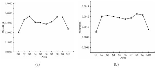
Figure 5.
(a) The total mass of particles in each area in the simulation at 60 s. (b) The average cumulative wear of each area in the simulation at 60 s.
4.2. Analysis of the Influence on Liner Wear by Particles with the Same Quality
To further verify the influence of the particle mass distribution on the non-uniform wear of the liner, this study also carried out a counter-evidence simulation. In the counter-evidence simulation, the simulation time was set to 40 s, and the particles of different densities generated in the cylinder were adjusted to particles with the same mass and different sizes; other simulation parameters remained unchanged. The line graph of the total mass distribution of particles in each area and the curves of the average cumulative wear under this condition are shown in Figure 6a,b.
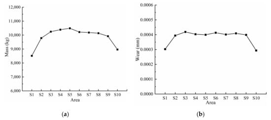
Figure 6.
(a) The total mass of particles in each area in the simulation at 40 s. (b) The average cumulative wear of each area in the simulation at 40 s.
Since the mass of all particles was the same, there was no big difference in the total mass of the particles in each area of the cylinder, but it could still be observed that the total mass curve of the particles in the middle of the cylinder showed a slight convexity; that is, the particle density in the middle of the cylinder was higher. Similarly, in the average cumulative wear curve, the wear of each area was relatively uniform except for Areas 1, 10, which meant that under the condition of the same quality of particles, there would be no obvious stratification and the wear of the liner became uniform. From this, we can infer that the difference in the quality of the particles in the cylinder causes the non-uniform distribution of particles in each area so that the total mass of the particles in each area is different, which ultimately causes the difference in wear in each area of the liner.
4.3. Variation of the Distribution of Particle Compositions in Each Area of the Cylinder
During the operation of the SAG mill, the total mass of particles in each area of the cylinder had changed; that is, the particles had stratified. To further study the distribution of particles, a graph to describe the number of particles in different areas at different time points was drawn for eight kinds of particles in the cylinder.
The rock particles in the simulation were not directly spherical, but were composed of multiple spherical surfaces according to actual working conditions. Eight kinds of particle mass are shown in Table 2. The number and mass of various kinds of particles in each area at the four time points of 30 s, 40 s, 50 s, and 60 s were comprehensively counted. Based on this, the distribution graph of various kinds of particles in various regions at different time points was drawn.
Table 2.
Each kind of particle mass and the proportion of these particle masses to the total mass.
As shown in Figure 7a, in the analysis of the various kinds of particles according to the individual particle mass from large to small, it can be found that for the largest mass of steel balls with a particle size of 150 mm, the number peaks mostly appeared in Areas 1, 2, and 10; the valley was in Area 6. The average extreme value at each time point, relative to the total number, accounted for 6%, and the maximum extreme value relative to the total number accounted for 9%. The number of this kind of particle in the feed end area was slightly more than that in the discharge end area at each time point.
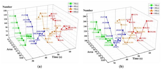
Figure 7.
(a) The number of 150 mm steel balls distributed in each area at each time point. (b) The number of 130 mm steel balls distributed in each area at each time point.
As shown in Figure 7b, for steel balls with a particle size of 130 mm, the peak numbers of the balls mostly appeared in Areas 2, 3, 9, and 10, and the valleys were in Areas 5 and 6. The average extreme value at each time point, relative to the total number, accounted for 6%, and the maximum extreme value relative to the total number accounted for 9%. The number of this kind of particle distributed in the feed end area at each time point was slightly more than the number in the discharge end area.
As shown in Figure 8a, for rocks with a particle size of 200 mm, their peak number appeared in Areas 9 and 10, and the valley was in Area 5. The average extreme value, relative to the total number at each time point, accounted for 5.1%, and the maximum extreme value relative to the total number accounted for 6%. The number of particles distributed in the discharge end area at each time point was more than the number in the feed end area.
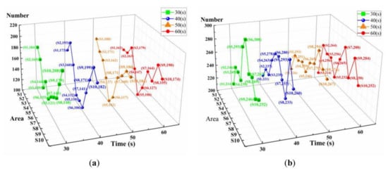
Figure 8.
(a) The number of 200 mm rocks distributed in each area at each time point. (b) The number of 110 mm steel balls distributed in each area at each time point.
As shown in Figure 8b, for steel balls with a particle size of 110 mm, the peak number was mostly in Areas 6 and 7, and the valley was in Area 1. The average extreme value, relative to the total number at each time point, accounted for 1.8%, and the maximum extreme value relative to the total number accounted for 3.6%. There was no significant difference in the number of particles at the discharge end and feed end areas.
As shown in Figure 9a, for the rocks with a particle size of 180 mm, the peak number was mostly in Areas 3 and 8, and the valley was in Area 6. The average extreme value at each time point, relative to the total number, accounted for 1.2%, and the maximum extreme value relative to the total number accounted for 2.9%. There was no significant difference in the number of particles at the discharge end and feed end areas.
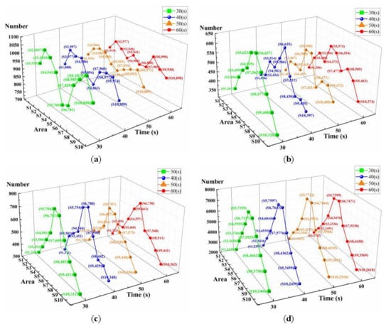
Figure 9.
(a) The number of 180 mm rocks distributed in each area at each time point. (b) The number of 90 mm steel balls distributed in each area at each time point. (c) The number of 70 mm steel balls distributed in each area at each time point. (d) The number of 60 mm rocks distributed in each area at each time point.
As shown in Figure 9b–d, for steel balls with a particle size of 90 mm, steel balls with a particle size of 70 mm, and rocks with a particle size of 60 mm, the peak numbers of these kinds of particles all appeared in Areas 5 and 6, and the valley was in Areas 1 and 10. The average extreme value of each particle at each time point, relative to the total number, accounted for 4.6%, 8%, and 10.8%, respectively, and the largest extreme value relative to the total number accounted for 6.6%, 9.2%, and 11.1%, respectively. There was no significant difference in the number of particles at the discharge end and feed end areas.
Based on this result, the following inference can be made: the reason for the non-uniform distribution of particles comes from the conical structure of the end covers on both sides of the SAG mill. Because the conical structure exerts an axial force on the particles, the particles of different masses have different axial velocities. Lightweight particles will be easily thrown to the middle of the cylinder, while large particles will accumulate on both sides of the cylinder.
When the water ingress factor was not considered in the simulation, and the taper of the two end covers was completely the same, the distribution of the particles was mostly axially symmetric. However, the slight deviation in the number of the two ends with the steel ball with a particle size of 150 mm and the rocks with a particle size of 200 mm was likely to be caused by more accidental factors in the particle motion simulation and the difference in the structure of the end covers.
It can be seen from Table 2 that the rocks with a particle size of 180 mm had the largest mass proportion, and their distribution was relatively uniform except for the discharge end and feed end. This ensured that there would be no significant differences in the wear of the cylinder liner in each area along the axial direction. Since the cumulative height of the particles in each area would not be too different, the areas where large mass particles were accumulated, namely Areas 2, 3, 8, and 9, had higher particle densities than other areas, the impact kinetic energy of the particles was also greater, and the wear would be greater. This kind of particle stratification caused by the cylinder structure is the reason for the non-uniform wear of the cylinder liner. The accumulation of large particles on both sides of the cylinder was not conducive to the discharge of rock, and it was easy to cause jams and the accumulation of stubborn stones.
5. Conclusions
By refining the kinds and shapes of steel balls and rock particles, collecting data on the spot, and constructing a complete cylinder model, the simulation results can be restored to the actual scene as much as possible. Based on these works, a simulation study on the non-uniform wear along the axial direction of the cylinder liner in a large-scale SAG mill was carried out, and the following conclusions were drawn:
- The non-uniform wear along the axial direction of the cylinder liner in the large-scale SAG mill was caused by the stratification of particles during cylinder operation and the difference in the total mass of the particles in each area;
- The stratification of particles along the axial direction was the inevitable result of the conical structure of the feed end cover and the discharge end cover. With the high-speed rotation of the cylinder, the particles were thrown to the middle of the cylinder under the influence of the end cover. Large particles could only be thrown down to both sides of the cylinder, while particles with small masses were concentrated in the middle of the cylinder. As a result, the impact energy and impact density of each area of the liner along the axial direction were different, which ultimately produced the non-uniform wear of the liner along the axial direction;
- By analyzing the data of each kind of particle one by one, it was found that when the mass of a single particle was below 3 kg, the particles would have obvious accumulation in the middle, and the lighter the mass, the greater the accumulation. When the mass of a single particle was about 6 kg, the particle distribution was the most uniform. When the mass of a single particle was greater than 10 kg, this kind of particle would accumulate on both sides of the cylinder, making the wear in these areas larger than in other areas. More importantly, this effect would begin to appear in the first few laps of the SAG mill and would continue to affect work efficiency until the end of the work. Therefore, when the SAG mill is configured, the main crushed particles (that is, the rocks with a particle size of 180mm in this study) should be distributed as evenly as possible throughout the cylinder;
- The particles were affected by the conical surfaces on both sides of the cylinder, and the number of particles distributed in Areas 1 and 10 was relatively small, so the total mass and wear of the particles in Areas 1 and 10 were always the smallest;
- The accumulation of large mass particles on both sides increased the wear of the liner and also affected the discharge, which increased the possibility of jams and stubborn stone accumulation.
Author Contributions
Conceptualization, H.C.; formal analysis, H.C. and Q.H.; methodology, W.W., H.C., and Q.H.; resources, W.W.; writing—original draft preparation, H.C.; writing—review and editing, H.C. and Q.H.; supervision, W.W.; project administration, H.C. All authors have read and agreed to the published version of the manuscript.
Funding
This research work is supported in part by the National Natural Science Foundation of China (Grant No. 51774340), in part by the research program of the State Key Laboratory of High Performance Complex Manufacturing (Grant No. zzyjkt201503), and in part by the Scientific Research Fund of the Hunan Provincial Education Department (Grant No. 19B299).
Conflicts of Interest
The authors declare no conflict of interest.
References
- Jnr, W.V.; Morrell, S. The development of a dynamic model for autogenous and semi-autogenous grinding. Miner. Eng. 1995, 8, 1285–1297. [Google Scholar]
- Lakshmanan, V.I.; Ojaghi, A.; Gorain, B. Beneficiation of Gold and Silver Ores. In Innovations and Breakthroughs in the Gold and Silver Industries; Springer: Cham, Switzerland, 2019; pp. 49–77. [Google Scholar]
- Shiliang, Y.; Baodong, Y.; Longde, L.; Xiaoli, G.; Yue, W. Exploration of application of SABC process in domestic production practices. Gold 2013, 3, 19. [Google Scholar]
- Chandramohan, R.; Powell, M.S. A structured approach to modelling SAG mill liner wear–monitoring wear. In Proceedings of the International Autogenous and Semiautogenous Grinding Technology, Vancouver, Canada, 23–27 September 2006; University of British Columbia: Vancouver, BC, Canada, 2006; pp. 24–27. Available online: https://www.researchgate.net/profile/Malcolm_Powell/publication/43498056_A_structured_approach_to_modelling_SAG_mill_liner_wear_-_monitoring_wear/links/58afac92a6fdcc6f03f358c8/A-structured-approach-to-modelling-SAG-mill-liner-wear-monitoring-wear.pdf (accessed on 26 November 2020).
- Weidenbach, M.; Griffin, P. Liner optimisation to improve availability of the Ridgeway SAG mill. In Proceedings of the Ninth Mill Operators’ Conference, Fremantle, Australia, 19–21 March 2007; The Australasian Institute of Mining and Metallurgy: Carlton, Australia, 2007. [Google Scholar]
- Banisi, S.; Hadizadeh, M. 3-D liner wear profile measurement and analysis in industrial SAG mills. Miner. Eng. 2007, 20, 132–139. [Google Scholar] [CrossRef]
- Yahyaei, M.; Banisi, S. Spreadsheet-based modeling of liner wear impact on charge motion in tumbling mills. Miner. Eng. 2010, 23, 1213–1219. [Google Scholar] [CrossRef]
- Yahyaei, M.; Banisi, S.; Hadizadeh, M. Modification of SAG mill liner shape based on 3-D liner wear profile measurements. Int. J. Miner. Process. 2009, 91, 111–115. [Google Scholar] [CrossRef]
- Mishra, B.K.; Rajamani, R.K. The discrete element method for the simulation of ball mills. Appl. Math. Model. 1992, 16, 598–604. [Google Scholar] [CrossRef]
- Cleary, P.W. Charge behaviour and power consumption in ball mills: Sensitivity to mill operating conditions, liner geometry and charge composition. Int. J. Miner. Process. 2001, 63, 79–114. [Google Scholar] [CrossRef]
- Toor, P.; Bird, M.; Perkins, T.; Powell, M.; Franke, J. The influence of liner wear on milling efficiency. Proc. Metplant 2011, 2011, 193–212. [Google Scholar]
- Cleary, P.W. Axial transport in dry ball mills. Appl. Math. Model. 2006, 30, 1343–1355. [Google Scholar] [CrossRef]
- Xu, L.; Luo, K.; Zhao, Y. Numerical prediction of wear in SAG mills based on DEM simulations. Powder Technol. 2018, 329, 353–363. [Google Scholar] [CrossRef]
- Zhang, X. Performance Analysis of Ball Mill Liner Based on DEM-FEM Coupling. Adv. Manuf. Autom. 2020, 634, 3. [Google Scholar]
- Herbst, J.A.; Nordell, L. Optimization of the design of sag mill internals using high fidelity simulation. In Proceedings of the SAG Conference, Vancouver, Canada, 30 September–3 October 2001; University of British Columbia: Vancouver, BC, Canada, 2001; Volume 4, pp. 150–164. [Google Scholar]
- Cleary, P.W.; Owen, P. Effect of operating condition changes on the collisional environment in a SAG mill. Miner. Eng. 2019, 132, 297–315. [Google Scholar] [CrossRef]
- Archard, J.F. Contact and rubbing of flat surfaces. J. Appl. Phys. 1953, 24, 981–988. [Google Scholar] [CrossRef]
- Xu, L.; Bao, S.; Zhao, Y. Multi-level DEM study on liner wear in tumbling mills for an engineering level approach. Powder Technol. 2020, 364, 332–342. [Google Scholar] [CrossRef]
- Li, T.; Peng, Y.; Zhu, Z.; Zou, S.; Yin, Z. Discrete element method simulations of the inter-particle contact parameters for the mono-sized iron ore particles. Materials 2017, 10, 520. [Google Scholar] [CrossRef] [PubMed]
- Morrell, S. Predicting the specific energy of autogenous and semi-autogenous mills from small diameter drill core samples. Miner. Eng. 2004, 17, 447–451. [Google Scholar] [CrossRef]


Publisher’s Note: MDPI stays neutral with regard to jurisdictional claims in published maps and institutional affiliations. |
© 2020 by the authors. Licensee MDPI, Basel, Switzerland. This article is an open access article distributed under the terms and conditions of the Creative Commons Attribution (CC BY) license (http://creativecommons.org/licenses/by/4.0/).