Abstract
Background: With the ever-increasing availability of data and a higher level of automation and simulation, production scheduling in the factory for prefabrication can no longer be seen as an autonomous solution. Concepts such as building information modelling (BIM), graphic techniques, databases, and interface development as well as heightened emphasis on overall-process optimization topics increase the pressure to connect to and interact with interrelated tasks and procedures. Methods: The automated optimization framework detailed in this study intended to generate optimal schedule of prefabricated component production based on the manufacturing process model and genetic algorithm method. An extraction and segmentation approach based on industry foundation classes (IFC) for prefabricated component production is discussed. During this process, the position and geometric information of the prefabricated components are adjusted and output in the extracted IFC file. Then, the production process and the completion time of each process have been examined and simulated with the genetic algorithm. Lastly, the automated optimization solution can be formed by the linking production scheduling database and the computational environment. Results: This shows that the implementation of the automated optimization framework for the production scheduling of the prefabricated elements improves the operability and accuracy of the production process. Conclusions: Based on the integration technique discussed above, the data transmission and integration in the mating application program is achieved by linking the Python-based application, the Structured Query Language (SQL) database and the computational environment. The implementation of the automated optimization framework model enables BIM models to play a better foundational role in patching up the technical gaps between prefabricated building designers and element producers.
1. Introduction
While the traditional construction industry has brought great changes to social activities, it is characterized by low productivity, a poor production environment, and high safety risks. The prefabricated building, a major feature of which is factory production, is a substantial revolution for the construction industry. The prefabricated components are produced in prefabrication plants mainly by assembly-line production, the long-line-method pedestal production, and fixed die table production. However, problems such as a shortage of skilled labor, the aging of workers, limited production capacity, and technological standards have hindered the development of the industry in recent years [1]. There is a pressing need to reexamine current practices so that the yield can be maximized with the same inputs and costs while maintaining production quality at a satisfactory level [2].
For the completion of prefabrication production, the effective integration of design drawings/models, production scheduling, and the assembly scheme must be considered [3,4]. As in any supply chain, information extraction and sharing among different production stages in prefabrication factories are important for efficient logistics and production scheduling [5]. As widespread digital tools used in the architecture, engineering, and construction (AEC) industry, building information modeling (BIM) technologies are expected to facilitate the collaboration between component manufacturers and designers; moreover, production scheduling optimization can be achieved in the BIM environment [6].
Within the field of production management, scheduling, as a decision-making process, makes great contributions to the provision of optimal solutions to one or more objectives associated with resource allocation. Typically, during the production process of prefabricated components, there remains a deficiency in the automatic extraction of effective information from architectural and structural models to support manufacturing process design and production scheduling. It must be noted that architectural/structural design is essentially a concept of the fabricated components that are meant to satisfy the functional objectives of a building. In the manufacturing plant, adjustments and segmentation considerations must be made for the transformation from architectural design to the processing of design components [7,8]. Specifically, traditional solutions to the manufacturing process, including the model construction of prefabricated components and the manual extraction of inherited properties from architectural design models, often cause a reduction in production efficiency. Moreover, due to the different temporal requirements of the manufacturing processing of prefabricated components, production scheduling must be optimized to reduce the waiting time of the production queue and workers’ free time. Li et al. and Jeong et al. [9,10] indicated that the prefabricated component information in the industry foundation classes (IFC) data model can be effectively extracted and classified, which could improve production management efficiency. Among the recognized research gaps, standards-compliant interoperability and integration between manufacturing processes and design model systems are of considerable importance [8,11].
To produce prefabricated components, the process model and corresponding geometric properties must be fully described. The detailed specifications of prefabricated components, such as their overall dimensions and materials, are commonly provided by BIM. It should be noted that in an automated environment, the production process model is generated by extra operations on three-dimensional design models, such as model recognition, extraction, and segmentation, which can quickly index shapes and support fast data access [12,13]. Although BIM provides detailed specifications of construction-oriented products, the integration of BIM with manufacturing process design remains under development [14]. At present, the lack of integration between manufacturing and BIM is overcome by means of expert knowledge and experience in different domains, which creates a barrier that inhibits information exchange between product designers and manufacturers, and increases production costs due to the increased communication [8]. Referring to the current limitations and problems, two solutions, namely commercial software, and IFC-based program development, are available to directly export dimensional data and generate process models regarding manufacturability. Firstly, commercial BIM software allows related functions and operations to be realized in their own operation platforms. In contrast, IFC files, as a basic generalized file-based means, will provide a more reliable solution for integration and invocation in the manufacturing management system. Thus, related issues may arise from manufacturing management systems, namely production delays and difficulties in generating production processing models in non-commercial software platform environments. Consequently, an automated, text-content-based, and satisfactory solution for the production of prefabricated components is increasingly in demand.
The remainder of this paper covers five aspects. Firstly, the existing research related to production scheduling and IFC model segmentation is presented. After the literature review, the employed method is proposed. Thirdly, an IFC-based extraction and segmentation approach for the production of prefabricated components is discussed. During this process, the position and geometric information of the prefabricated components are adjusted and output in the extracted IFC file. Then, the production process and the completion time of each process are examined and simulated with the genetic algorithm. Finally, the automated optimization solution can be formed by linking the production scheduling database and the computational environment.
2. Related Works
2.1. Production Scheduling of Prefabricated Elements
With the rapid development of prefabricated buildings in China, prefabricated construction factories have emerged, and some processes have been automated with a manufacturing-like production line model. Hence, prefabricated elements are produced according to orders (made-to-order, MTO), which imposes strict time limits from order to delivery. Considering this problem, many scholars have developed various models or algorithms to optimize production scheduling. Regarding dispatching, Li et al. [15] identified the challenging dispatching problem, modeled it as a unique type of vehicle routing problem with time windows (VRPTW), and addressed this issue by utilizing an improved artificial bee colony (IABC) algorithm. Kim et al. [16] adopted a discrete-time simulation method to cope with due date changes in real-time and proposed a new dispatching rule that considers the uncertainty of the due dates to minimize tardiness. Ko and Wang [17] developed a multi-objective production scheduling model (MOPPSM) that considers production resources and the buffer size between stations, as well as a multi-objective genetic algorithm to determine the minimum makespan and tardiness penalties. Similarly, Wang et al. [18] proposed a multi-agent-based planning model to synchronize production scheduling and resource allocation. Based on this, on-time delivery, minimum waiting, and time extensions are available via the utilization of the heuristic algorithm to integrate the optimization techniques.
Among the algorithms available for the optimization of production scheduling, the genetic algorithm (GA) has attracted substantial attention and has been greatly improved in recent years. Leu and Hwang [19] adopted a GA-based searching technique in a scheduling system to optimize production sequences, resource utilization, and the minimum makespan. Based on this, Anvari [20] firstly adopted a GA-based optimization approach to solve a holistic maximum task assignment (MTA) problem to minimize the time and cost while maximizing safety. Wang et al. [21] established a two-hierarchy simulation-GA hybrid model for prefabricated production (TSGH_PP) to navigate the uncertainty in processing time in practice, and the process-waiting time on the flow of work. As a result, the trade-off between the on-time delivery of prefabricated components with conflicting purposes can be achieved, thereby minimizing the production cost, and resource configuration can be optimized. However, there has been little research on optimized scheduling production while considering both the GA and application of BIM; specifically, the use of IFC extraction and automated text analysis to improve the operability of IFC model segmentation and its application in IFC standards-supporting environments has not been investigated.
2.2. IFC Extraction and Automated 3D Model Split
The management of prefabricated components requires intensive information exchange between the factory and construction site to synchronize the production of prefabricated elements, transport, and elements assembly. As a useful tool, BIM technology can be integrated into the construction of prefabricated buildings. The most notable and widely accepted product data model for BIM is the IFC-based model, which is an open standard for the exchange of building data models used in the AEC industry across different software to improve collaboration on building projects [22]. Determining how to effectively extract specific information from the building information model and conduct automated 3D model segmentation has become an obstacle to the facilitation of effective operations with spatial models [12].
According to different recognition algorithms, various information extraction techniques have been proposed. Chen et al. [23] developed a web information server based on the IFC standard with web and XML (Extensible Markup Language) technology for collaboration and information sharing to extract some models required for structural analysis. Nepal et al. [24] analyzed the geometric and topological relationships between BIM model components represented by IFC to identify structural features and inferred the process of structural feature extraction. This research provided a substantial reference for component extraction. To reduce the production, transportation, and installation costs, the total number of components must be controlled; this requires an IFC-based system to configure the grouping of prefabricated components. Essentially, the framework developed by Khalili et al. [25] was designed to extract the topological relationships and geometric properties of building elements from the IFC file. Similarly, Zhang et al. [26] described an ontology-based partial model extraction approach by applying semantic technology and used the ontology-augmented model index to successfully extract a portion of the building information model from the complete IFC model.
At present, visualization technology can generate extremely accurate and high-quality structural 3D models. However, the ability to directly and accurately extract and segment these models remains limited. To improve 3D model segmentation performance, Baldacci et al. [27] presented a 3D split-and-merge segmentation method using topological and geometric structuring with an oriented boundary graph, which may be optimized by parallel algorithms. Zhu et al. [28] developed an approach to convert various types of 3D models into BREP (Boundary Representation) models and then perform model segmentation. Similarly, Marras et al. [29] proposed a hybrid method, called the Adaptive Geometric Split Merge (AGSM) segmentation algorithm, which exploits both the region shape and data value characteristics to find the maximum homogeneity axis of the volume, and ultimately to divide the entire volume into several large homogeneous 3D regions.
In summary, in order to use BIM as the source of design and production information for current production schedule design, a system is needed to automatically determine the geometric dimensions for the production process model, and to facilitate schedule planning for multi-task-oriented manufacturing arrangements.
3. Methodology
The proposed system aims to determine if the manufacturing process model of building component assembly can be extracted from the architectural design model and arranged production schedule via an automated optimization framework that integrates BIM and the given optimization algorithm. The proposed system is presented in Figure 1, and the architecture can be divided into three modules: ① the identification, extraction, and segmentation of an IFC data file designed for the production of prefabricated components; ② the implementation of the GA; ③ the implementation of processing and calculation.
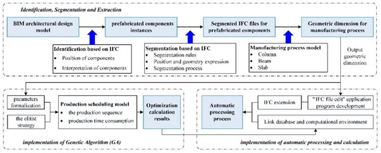
Figure 1.
Overview of the proposed automated optimization system.
In the proposed framework, three modules are applied sequentially. Firstly, the IFC data file module involves the identification and extraction of prefabricated component instances from a pre-designed text-based IFC file. The IFC physical file is then segmented to generate a manufacturing process model of selected columns, beams, or slabs according to different production technique specifications. In the identification process, the prefabricated component instances are generated based on the positioning of the target components and interpretation of the component properties. The proposed segmentation framework is achieved by developing the IFC file editing application program in the Python language. The segmented IFC files for prefabricated components contain the geometric dimension information required in the manufacturing process. A manufacturing schedule, as the best possible near-optimal solution, is often acceptable. Therefore, in the GA implementation stage, a mathematical model of the optimization of the production schedule of prefabricated components is of necessity. This paper therefore presents a scheduling approach based on the GA that is developed to address the scheduling problems in manufacturing systems constrained by both production sequences and time consumption. The GA utilizes a chromosome representation, which takes into account both machine and worker assignments to produce prefabricated columns, beams, and slabs. Moreover, the elitist-population strategy-based GA has been demonstrated to be greatly efficient and effective in finding multiple solutions to manufacturing scheduling optimization problems. In the automatic processing and calculation stage, the MySQL database is employed to obtain production time parameters from the IFC file editing application. The results of production scheduling optimization are then generated and displayed in the automatic environment by linking MySQL and MATLAB. Upon completion of this stage, the user of the proposed framework will have a clear understanding of how the manufacturing schedules of prefabricated components can be arranged.
4. IFC-Based Extraction and Segmentation of Prefabricated Components
4.1. Component Identification and Extraction Based on the IFC Schema
The identification of prefabricated component information refers to the positioning of the target components and the interpretation of component properties. The positioning of the target components is the precondition for further component data identification. By interpreting the spatial structure hierarchy for the elements of a building project and specifying the target component, the distinguishing attributes can be identified. An IFC file represents a directed graph with edges for forward and inverse attributes. The general attributes are expressed according to the sequence of attribution definition. By querying the relationship entities, the attribute information of the building components can be parsed and identified.
The algorithm proposed in this paper generates the element model by iteratively extracting IFC data instances in referential relations directly from an IFC instance model file, and it relies solely on the internal data structure of the IFC instance model. The algorithm firstly detects the IFC entities corresponding to selected building elements. It then extracts physical and nonphysical data instances relevant to the user’s selection of building elements by iterating through data instances based on the rules specified in the algorithm until all related data instances are extracted (Won et al. 2013). Figure 2 illustrates the extraction algorithm, which is divided into seven steps.
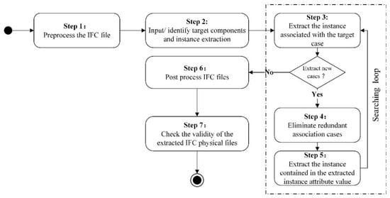
Figure 2.
Component extraction based on the industry foundation classes (IFC) physical file.
- (1)
- Preprocessing of the IFC physical file
To query and extract attributes in the IFC physical data file via programming, it is essential to preprocess the IFC file and segment the strings according to the instance name, entity name, and entity attribute defined in the STEP (Standard for the Exchange of Product Model Data) language. As shown in Figure 3, the attributes are separated by “.” in the string, and are stored as a text file for further utilization.
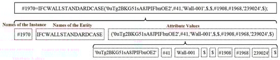
Figure 3.
IFC physical file segmentation of a wall entity.
- (2)
- Identifying and Extracting Target Components
Firstly, the categories of the target components, such as walls, slabs, beams, columns, or stairs, are specified. Then, the programming will traverse the IFC physical data file to detect the corresponding IFC entities through the predefined mapping relationships. Figure 4 presents an example of IfcWallStandardCase extraction.
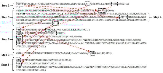
Figure 4.
Iteration of component extraction based on the IFC physical file.
- (3)
- Extracting the Relation Entities of Target Components
After the IFC physical file is processed, the attributes of the target entities will be traversed and queried. As represented in Figure 4, the target entity #1970 is connected with building story entity #115 through relational entity #270685, IfcRelContaninedInspatialStructure. Therefore, to discover the relationships between entities, the relational entities, which have the prefix IfcRel, will be specified. Among them, IfcRelAggregates describes the relationships between buildings, sites, projects, and building stories. Moreover, IfcRelContainedInSpatialStructure represents the relationships between different spatial elements. The programming will loop through the physical data file until no more new entities are detected. To improve the retrieval efficiency, after the first loop, new entities will first be compared to the extracted entities before querying the entire IFC file.
- (4)
- Eliminating Redundant Relational Entities
This step aims to filter the unselected relational entities contained in the target component entities to reduce the number of extracted entities. In Figure 4, the relational entity #270685 contains the target entity #1970, and indicates the spatial relation of target entity #1970 and building story entity #115. The relational entity #270685 also refers to 48 non-target entities, such as #256, #378, #449, etc., which must be eliminated.
- (5)
- Extracting the Entities Contained in the Selected Attributes
The entities contained in the attributes of extracted entities will be retrieved. If the entity has already been extracted in the previous loop, it will be skipped. The new entities extracted in step 5 will be processed as the target entities in step 3 of the next loop. In the first loop, the combination of the target entities in step 2 and the filtered entities in step 4 is selected as the entities input in step 5. In the following loops, the entities input in step 5 should consist of the entities extracted in step 5 of the previous loop and the filtered entities in step 4 of this loop. Figure 4 shows that the processing in step 5 of the second loop will extract entities #41, #1908, #1968, #2094, #115, and #160, as well as entity #38, which is included in #41.
- (6)
- Postprocessing after Extraction of the IFC Physical Data File
As the extracted IFC entities are stored in a text-based structure, the separate entity name, instance name, specific signs, and attributes could constitute the data segments in the plain text file. According to the IFC physical file format defined by the STEP language, the file header of the original file will be preserved.
4.2. Prefabricated Component Segmentation Based on the IFC Standard
4.2.1. Segmentation Rules
It is of great importance to divide precast and cast-in-place segments of prefabricated elements in a complete BIM model according to the task requirements that may occur in the design, manufacturing, and construction stages. Generally, the external factors of concern in prefabricated component segmentation primarily include the characteristics of the building structure, prefabrication rate, assembly sequence planning, force distribution, production specifications, assembly precision, and size limitation of transportation and hoisting. This study mainly discusses the direct segmentation method based on the extracted column, beam, and slab elements from the IFC physical data file. The proposed approach is processed to deal with the linkage rules of prefabricated element nodes, and a specific IFC physical data file of precast segments is formed. The linkage of the precast column, beam, and slab elements is presented in Figure 5, and the manufacturing and construction details are as follows.
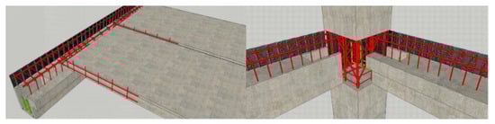
Figure 5.
Schematic diagram of the lap joints of prefabricated members.
(1) Columns: the prefabricated column is located 20 mm above the baseboard. The top of the column reaches the bottom of the beam. The two parts of the column are connected by grouting in the sleeve.
(2) Beams: beams consist of prestressed composite beams and ordinary composite beams. There is a 10 mm overlap in the joint with the adjacent column. The top of the beam has the same height as the bottom of the slab.
(3) Slabs: the prestressed composite slab has a 10 mm deep lap with the adjacent beam. If unidirectional prestressed concrete composite slabs are adopted, then they can lay close to each side with extra reinforcing steel assigned in the edge joint. If unidirectional, prestressed, two-way concrete composite slabs are adopted, the non-prestressed steels between adjacent slabs should stretch out and be spliced together. The width of late-poured bands should not be less than 200 mm, and the thickness of the prefabricated part of the composition slab should be more than 60 mm.
4.2.2. Position and Geometry Expression in IFC Schema
In the IFC schema, the attribute “Representation” generally describes the geometry, and the attribute “ObjectPlacement” describes the position information. The specific expression of the position and geometry in column, beam, and slab elements is discussed as follows.
(1) Columns: Figure 6 shows the position of entity #152 in a three-level nested layer structure. When extruding the column element, its coordinate system is determined by the entity IfcLocalPlacement and its coordinate value is given by the related entity IfcCartesianPoint.
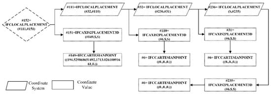
Figure 6.
Example of position expression.
As shown in Figure 7, the geometric information of column entities in the IFC physical data file is defined in two ways, namely mapping definition, and direct definition. In the IFC schema, IfcMappedItem is the inserted instance of a source definition to be mapped with target instances that have the same geometric shapes. IfcMappedItem can reuse other mapped items based on an IfcShapeRepresentation, including one or more IfcMappedItem. The transformation is defined by entity IfcCartesianTransformationOperator to achieve the operations of translation, rotation, mirroring, and zoom. On the other hand, in direct definition, the target instance can directly quote the geometric expression of the existing instances without the mapping process. The geometric information, including the profile section, cardinal point, extruded direction, and length, is described by IfcExtrudedAreaSolid. In Figure 7, #126 defines the shape of the section as a rectangle; #127 reveals the initial position; #19 describes the extrusion direction, which is 4000 for this column.
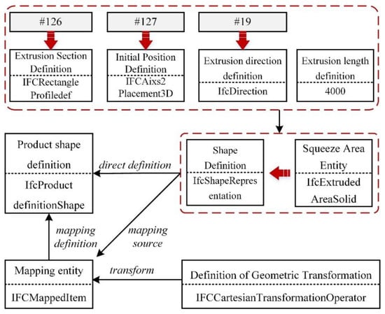
Figure 7.
Example of column geometry expression.
Figure 8 shows the detailed shape and position definition described by the entity IfcExtrudedAreaSolid. For the relocation in the stretch process, the reference point of the column element is assigned by the entity IfcCardinalPointEnum, and then coincides with the coordinate origin of the stretch section provided by the entity IfcExtrudedAreaSolid. Therefore, by editing the attribute value of the stretch section, the changes in the size, position, and length of the stretch section in the IFC entity can be realized by editing the attribute values.
Figure 8.
Attributes of IfcExtrudedAreaSolid.
The segmentation of the column object is operated depending on the coordinate systems of the entity IfcExtrudedAreaSolid and other related entities. The extruded profile is set on the XY plane of the object coordinate system defined by the entity IfcLocalPlacement. For the standard rectangular column in Figure 9, the cardinal point of the column element in the IFC physical data file is defined as the central point of the bottom and is indicated by black lines. Additionally, “AXIS” in the column element should coincide with the extruded direction.
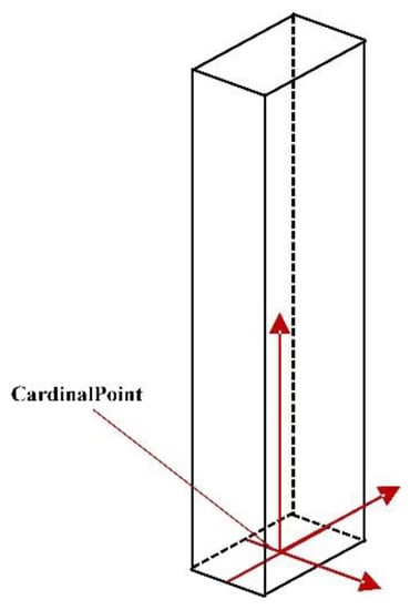
Figure 9.
Cardinal point in column element.
(2) Beams: the position information of the beam is given by the entity IfcLocalPlacement through coordinate values measured from the relative coordinate system in the nested layer structure. In the IFC schema, the beam element is also defined by “AXIS” and “BODY,” which express the 3D shape. The process of beam geometry representation is displayed in Figure 10. “AXIS” represents the axis parameter of a standard column, and “BODY” creates the 3D shape by SweptSolid or Clipping CSG (Constructive Solid Geometry). The axis is represented by the start and end-points in IfcPolyLine, which are given by entities #9 and #146. Entities #129, #132, and #19 constitute the source of the “BODY” definition for the beam geometry representation.
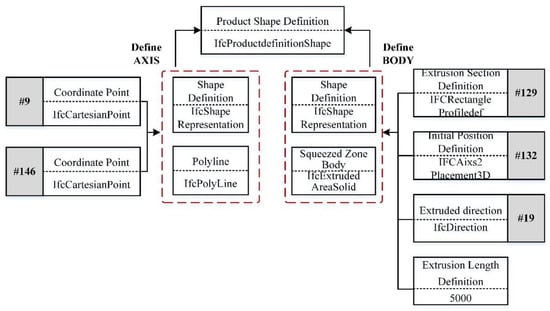
Figure 10.
Process of beam geometry representation.
Considering the standard rectangular beam in Figure 11, the cardinal point of the beam element in the IFC physical data file is in the upper center of the vertical profile, in contrast to the central-point position in the column element. Here, the black line represents the extrusion axis in the direction that is defined by IfcExtrudedAreaSolid and parallel to the Z-axis.
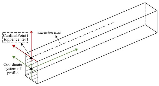
Figure 11.
Cardinal point in beam element.
(3) Slabs: the geometric information of the slab element is given by the class IfcExtrudedAreaSolid. The profile section of the slab that normally has a non-rectangular shape is defined by the entity IfcArbitraryClosedProfileDef, and the entity IfcPolyLine defines the curve. The profile is defined by an IfcPolyLine. The points defining the polyline are two-dimensional. As the profile must be closed, the last point in the polyline is the same as the first point. The underlying XY plane that sweeps the surface or the solid uses the coordinate system of the extruded profile. The base point of the profile is selected as the origin of the XY plane. The long edge and short edge from the bounding box of the extruded profile are, respectively, parallel to the X- and Y-axes. As shown in Figure 12, the closed bounded curve consists of 12 points, referring to the origin of its coordinate system.
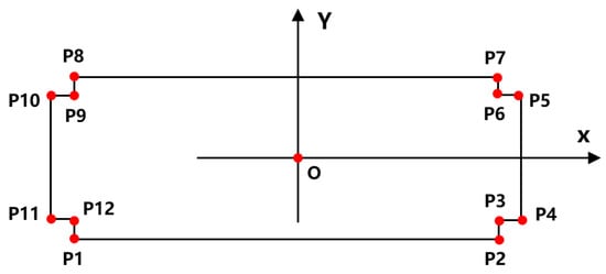
Figure 12.
Example of profile definition by entity IfcArbitraryClosedProfileDef.
4.2.3. Segmentation Process
As the lap connection design of the column, beam, and slab will affect the exported information of the IFC physical file, it is essential to specify the model rules as follows. ① For the frame structure, the column length is defined as the distance between the upper and lower floor slabs. Its profile is defined as the section perpendicular to its axis. ② The beam length is defined as the clear spacing between two columns or two main girders. Its profile is defined as the section perpendicular to its axis. ③ The length or width of a slab is defined as the distance between two associated beams. The slab thickness is given as the height of the section, which is perpendicular to its long edge and short edge. These rules are applied to all the column, beam, and slab models.
(1) Columns: the BIM model of a column includes the prefabricated part and cast-in-place part. As shown in Figure 13, to extract the precast beam that is in the middle of the element model, two cast-in-place parts must be eliminated. The upper part is formed from the bottom of the beam, and the lower part is the 10 mm cast-in-place part.
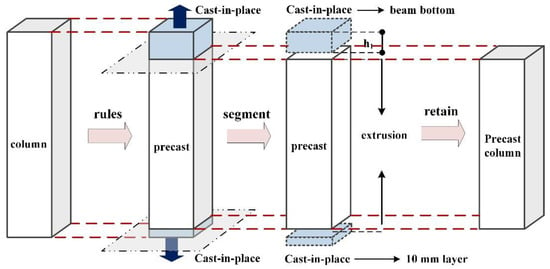
Figure 13.
Segmentation of a column.
The column segmentation in the physical data file is achieved according to the expression of the position and geometric information in the IFC file. By looping the position and geometric information through the IFC physical data file, all column entities will be identified. Firstly, explicit recognition of the position attribute, which is referred to by the sixth entity IfcLocalPlacement, and the geometric attribute, which is referred to by the seventh entity IfcProductionDefinitionShape, is conducted. Secondly, the second attribute IFCAxis2Placement3D and the first attribute IfcCartesianPoint in the entity IfcLocalPlacement are detected. Then, a 20 mm upward movement of the origin point in the column element is achieved by a 20 mm increase in the Z value, and the origin point is also viewed as the extrusion start point. Thirdly, the instances associated with the attributes in the entity IfcProductionDefinitionShape are retrieved, and the entity IfcExtrudedAreaSolid is confirmed. Then, (h1 + 10 mm) in the fourth attribute value, which represents height, is decreased; h1 is the thickness of the adjacent beam. Finally, the precast section of the beam model is extracted and divided from the cast-in-place part.
(2) Beams: the prefabrication of a beam can generally be processed as a two-story structure with cast-in-place and precast components. Figure 14 presents the general rule of precast beam segmentation; on the top level, a 10 mm thin precast layer against the adjacent slab needs to be eliminated, and, considering the production and construction requirements in practice, the precast part retained in the model at the bottom must be extended by 10 mm at both ends of the beam.
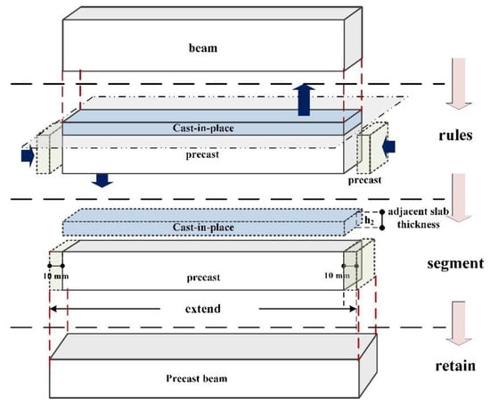
Figure 14.
Segmentation of a beam model.
The beam segmentation in the physical data file is achieved according to the position and geometric information expression in the IFC. By looping the position and geometric information through the IFC physical data file, all beam entities will be identified. Firstly, explicit recognition of the geometric attribute, which is referred to by the seventh entity IfcProductionDefinitionShape, is conducted. Secondly, the instances associated with the attributes in the entity IfcProductionDefinitionShape are retrieved and the entity IfcExtrudedAreaSolid is confirmed. Thirdly, the first attribute IfcRectangleProfileDef in instance IfcExtrudedAreaSolid is detected, then h2 in the fourth attribute value is subtracted; h2 is the thickness of the adjacent slab. Furthermore, the second attribute IfcAixs2Placement3D in the entity IfcExtrudedAreaSolid is specified, and the initial direction of the Z-axis defined by the instance is recognized; this is illustrated in Table 1. Then, the X-axis value of the first attribute IfcCartesianPoint in the associated instance is reduced by 10 mm, which changes the initial position of the beam entity. Finally, 20 mm is added to the fourth attribute in the entity IfcExtrudedAreaSolid to increase the beam length. Through the segmentation rules, the prefabricated beam can be created in the IFC physical data file according to the actual size required in precast manufacturing and construction.

Table 1.
Directions indicated by the second attribute of IfcExtrudedAreaSolid.
(3) Slabs: the 3D model of a slab can be formed by the precast and cast-in-place parts. The prefabrication of a slab can be generally designed as a two-segmentation process. Considering the production and construction requirements in practice, the general rule of precast beam segmentation, as shown in Figure 15, is that a thin cast-in-place layer on the top with a thickness of h3 is eliminated, and the precast part retained in the model is then extended by 10 mm on the four lateral sides of the slab.
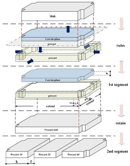
Figure 15.
Segmentation of the slab model.
In the slab model, the section properties are defined by the polyline and multiple points (shown in Figure 16). According to the segmentation rule of the prefabricated slab, a five-step process is adopted to calculate the vertexes, position information, and geometric information of the segmented slab.
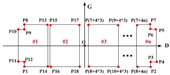
Figure 16.
Coordinates of the segmented slab.
Step 1: recognize the point instances included in the attributes of the entity IfcArbitraryClosedProfileDef, which is referred to by the entity slab, and extract the coordinate values of the point instances.
Step 2: identify the eight outer points P1, P2, P4, P5, P7, P8, P10, and P11 of the slab section in Figure 16. Select the points P10 and P11 with the minimum X-values, then subtract 10 from the X-values; the Y-values remain unchanged. Select the points P4 and P5 with the maximum X-values, then add 10 to the X-values; the Y-values remain unchanged. Similarly, find points P1 and P2 with the minimum Y-values, then subtract 10 from the Y-values; the X-values remain unchanged. Find points P7 and P8 with the maximum Y-values, then add 10 to the Y-values; the X-values remain unchanged. Afterward, the four lateral sides of the slab are extended by 10 mm.
Step 3: calculate and recognize the dimensions of the bounding rectangle of the slab section according to the positions of the adjusted coordinates. Assume and are assigned with the maximum X- and Y-values, and and are assigned with the minimum X- and Y-values, as shown in Equation (1).
Considering that a represents the long dimension of the bounding rectangle, and b represents the short dimension. If , then ; if , then . Correspondingly, in this study, D is utilized to direct the orientation of a longitudinal axis, and G is used to direct the orientation of a vertical axis. Thus, when , D and G are the X- and Y-axes, respectively; when , D and G are the Y- and X-axes, respectively.
Step 4: calculate and confirm the number of slab segments. In this study, k is used to denote the width of a standard slab with a lower limit k1 and upper limit k2, and f is the distance between two slab segments.
Step 5: after confirming the orientation of the long side of the slab section, the coordinates of the slab segments can be calculated. Figure 16 illustrates the G and D coordinates of the vertexes of the slab section. The rules are as follows. The slab segment containing the points with the minimum D-axis values is marked as the first slab segment (#1). Along the positive direction of the D-axis, the other slabs are regarded as the second (#2), third (#3) … n-th (#n) slab segments. If the D-axis is consistent with the X-axis, then P1, P2, P4, P5, P7, P8, P10, and P11 will first be recognized, and the corresponding coordinates can be calculated. If the D-axis is consistent with the Y-axis, then the coordinate system is rotated clockwise 90 degrees to recognize the eight points P on the edge of the bounding rectangle.
Slab segment #1 is formed by encircled points P1, P14, P13, P8, P9, P10, P11, and P12; the coordinates of P1, P8, P9, P10, P11, and P12 will remain unchanged after slab segmentation, while the coordinates of P13 (D, G) and P14 (D, G) are re-set via Equations (2) and (3).
Next, slab segment #2 is formed by encircled points P15, P16, P17, and P18, which are calculated by Equations (4)–(7).
Similarly, the bounding points of the i-th slab segment can be assigned as P(4i+7), P(4i+8), P(4i+9), and P(4i+10), where . The coordinate values of the i-th segment are deduced and calculated by Equations (8)–(11).
Finally, the n-th slab segment (#n) is associated with eight points: P(4n+8), P2, P3, P4, P5, P6, P7, and P(4n+7); the coordinates of P2, P3, P4, P5, P6, and P7 will remain unchanged after slab segmentation, while the coordinates of P4n+7 (D, G) and P4n+8 (D, G) are designed via Equations (12) and (13).
Slab segmentation in the IFC physical data file is achieved through the segmentation rules. By looping the position and geometric information through the IFC physical data file, all slab entities will be identified. First, n duplicated entities of the slab and its attributes are created, and n is determined by the coordinate access. Then, the slab entity number is updated and set as larger than all the other entity numbers in the IFC file. The reference of slab entities in the attribute entities is adapted to the updated entity number. Second, the entity IfcExtrudedAreaSolid is specified to refer to the slabs, and the coordinates in the entity IfcArbitraryClosedProfileDef are adjusted and aligned in the entity IfcPolyLine to adjust the slab profile. Third, the entity IfcExtrudedAreaSolid is specified to refer to the slabs, and its fourth attribute is decreased by h3 to ignore the cast part. As the original coordinate system and its reference point remain unchanged, the starting points of the slabs will be reserved after slab segmentation. Finally, the instance names of the geometric information in the slab attribute are updated.
5. An Automated Optimization Framework for Production Scheduling with the GA
As mentioned previously, the extraction and segmentation of prefabricated component models influence the accuracy of the production process model, which complicates the process of identifying the proper production schedule with different parameters. Hence, the utilization of an automated simulation-based optimization tool would be an appropriate approach to adjust these parameters. In this paper, the automated optimization process is presented in three stages, namely the data processing stage, data storage stage, and data application stage, as shown in Figure 17. In the data processing stage, the BIM model is constructed and exported in the form of an IFC physical file. The extraction and segmentation approach of the prefabricated component model is applied to generate component instances that meet the production process requirements of connection joints. IFC extension is used to express the production time parameter stored in the text-based physical files and then export it. In the data storage stage, a specific database is developed to manage the geometric attributes and production time parameters. In the data application stage, the GA model is implemented by linking the database and MATLAB to make a computing request and obtain the corresponding optimized schedule.
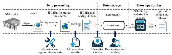
Figure 17.
Building information modelling (BIM) information transfer flow chart.
5.1. The Formalization of Production Scheduling Parameters
The production characteristics of prefabricated elements can be summarized by the following aspects. ① There are elements of multiple sizes in one project, and the number of elements of different sizes is different. ② For the same type of element, the production process is basically the same, but the production times of elements with different sizes and specifications in each process are different. ③ As the work content of each process differs greatly, the factory implements a pipeline operation in the management process, and the number of workers assigned to each process is different, while the work capacity of the same process is basically the same.
The hypotheses are therefore proposed as follows. The project has n types of elements, and the number of elements of each specification is . Each element has m operations, and the number of shifts in each operation is . X denotes a possible production plan (as given by Equation (14)), S denotes the total number of elements produced in Equation (15), and the k-th element in the first operation is denoted as . As the production sequence of the second process component is determined according to the end time of each element of the first process, which is different from the production sequence of the first process, the k-th element in the second process is denoted as , and the k-th element in the g-th process is denoted as .
Matrix T represents the processing time of each specification for each process, and denotes the production time of the element with the i-th specification in the g-th step, as shown in Equation (16).
For the production plan X, the element is denoted as at the g-th process by the b-th shift production completion time. In the shift groups produced at the same time in the g-th process, the earliest end time of the element is denoted as . After that, the first-ending shift group can be removed, and the latest end time of the component in the shift group of the g-th operation in the simultaneous production is denoted as [X].
The maximum completion time of the entire production plan is the end time of the element of the m-th operation and the maximum value of the completion time of other elements of the m-th operation. Therefore, in this paper, the optimization problem of production scheduling is to solve the minimum of . Then, due to the production sequence of different processes depending on the end time of the previous process, the production sequence of the second process corresponds to the sequence number k2. The completion time of the last process can be calculated utilizing matrix T.
5.2. GA Model Calculation of Production Scheduling
The production time–cost of prefabricated components can be organized as follows. Firstly, concrete pouring of the prefabricated components must be carried out continuously and completed within the working hours or the specified overtime. Then, the concrete maintenance must be completed during the non-working hours. Moreover, the start time of the next process should be in the working hours, so if the end time of concrete pouring is during a non-working hour, it will continue into the next day. Finally, other work should occur during the working hours and can be interrupted. The mathematical model is proposed as follows.
The factory’s daily working time is denoted as , the overtime is , and the non-working time is ; . For concrete pouring, the end time of component is described by Equations (17)–(19).
where is the production completion time, and is the production time of component in the g-th process. For concrete curing, the end time of component is described by Equations (20) and (21).
For the production process of other components, the end time of element is given by Equations (22) and (23).
The calculation process of the final completion time is shown in Figure 18 including two steps. Based on the initial component production sequence or the reordered sequence, the end time of the production of each component can be calculated separately. Considering the different processes, the results generated in the model can be input to the next process for calculation until the production of all components is completed, and the final production time can ultimately be determined.
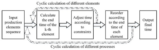
Figure 18.
Calculation of the final completion time.
With the parametric expression of production scheduling, an enhanced GA approach to search for optimum production schedules can be developed by utilizing the elitist strategy. The first step is to encode the specifications of prefabricated components, and the second step is to initialize the population. Elements are arranged in sequence to form an initial standard sequence, and the objective function and fitness function can then be, respectively, calculated. Then, a selection operator is used to choose chromosomes according to their fitness. The next step is crossing over, in which a random number between zero and one is generated for each pair of individuals and compared with the crossover probability to judge whether it crosses; the crossover probability is generally chosen between 0.44 and 0.99. In this work, it is firstly determined whether the chromosome needs to be mutated, two mutation points on the parent chromosome are randomly chosen, and the genes at the location of the mutation point are exchanged to achieve chromosome mutation. Finally, every generation contains elite solutions for better evolutions.
5.3. Experiment
In this research, a project in a prefabrication plant in Nanjing, China was taken as a case study to verify the proposed the GA-based production scheduling optimization method. The project required the factory production of prefabricated floors, beams, stairs, and balconies. According to statistics, this project contained a total of 74 precast slabs. Considering the slab size, column corner positions, and other factors, and ignoring the numbers of embedded parts and cavities, there were eight types of prefabricated floors, as shown in Table 2.
Table 2.
Types and quantities of precast slabs.
The factory divided the production process of the prefabricated components into five steps, namely: ① mold installation; ② rebar and embedded parts placement; ③ concrete placement; ④ the steam curing of concrete; ⑤ frame removal and inspection. The time–cost of the production process of each of the eight types of prefabricated slabs was collected, and is reported in Table 3. A production team was required to complete each production process in the scheduled time; a team refers to a group of workers assigned by the factory to complete the work according to the complexity of the work and the proficiency of the workers.
Table 3.
Operation times of different types of precast slabs (min).
- (1)
- Implementation of the GA for Production Scheduling
According to the established mathematical model and the GA discussed previously, MATLAB software was employed to calculate the loop iterations and simulate the final completion time . A portion of the core code is shown as follows in Algorithm 1.
| Algorithm 1 Completion time |
| 1: for i_process = 1: process_num 2: c = zeros (B(i_process),1); 3: for i_component = 1: component_num 4: [min_c,num_c] = min(c); 5: start_time = max(last_time(i_component,1),min_c); 6: end_time = start_time + T(last_time(i_component,2),i_process); 7: end_time = 8: check_time(end_time,type_list(i_process),TG,TJ,T(last_time(i_component,2),i_process)); 9: last_time(i_component,1) = end_time; 10: c(num_c,1) = end_time; 11: end 12: last_time = sortrows(last_time,1); 13: end |
The first step was to encode the component types with the symbols presented in Table 3 to form the chromosomes in the subsequent GA. For example, the production sequence of a certain precast slab was 21553672413141667478814352235111688616128385758887252855212282.
Furthermore, 352487522411 represents the production of one YLB-2L, then one YLB-1L, then two YLB-5Ls in that order, and finally one YLB-1L. The second step was to determine the population size P. To prevent falling into the local optimal solution or premature convergence, P was set as 50 based on the calculation by the GA after experiments. Then, the related parameters required in the experiment were set based on elitist selection; the retention rate was 0.02, the crossover rate was set as 0.95, and the mutation rate was 0.1. The program running environment was Windows 10, 64 bits, 8 GB memory, and MATLAB R016a. Finally, the algorithm was iterated 1000 times, which took 330.85 s, and the result was 7378 min. Figure 19 presents the variation of the optimal solution in each generation during the solution process. It was found that there was no solution to the minimum completion time. In this case, there was a total of 32 optimal production orders in the last generation of the calculation results.
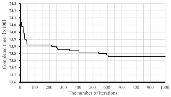
Figure 19.
Optimal solution of each generation in the iteration process of the genetic algorithm (GA).
The production time of prefabricated components between placing an order and the delivery of goods is usually limited, and the factory flexibly allocates the supply of resources according to the emergency of the order. The GA model used in this study can be applied with the parametric descriptions of the production team, working time, and other key resources to derive the optimal solution according to the completion time, and the allocation of resources can then be adjusted.
- (2)
- Implementation of the GA for production scheduling
To automatically acquire the attributes contained in the segmented parts of the BIM models of fabricated components for the calculation of production scheduling optimization, it is necessary to extend the IFC model to express attributes related to production scheduling optimization. In this study, considering that columns, beams, and slabs have been defined as entities in the IFC standard, the parameters of the production time could be extended to be the property set in the IFC model, as shown in Table 4. Each entity in the database is described by certain properties, which are pieces of information about an element that are required for processing performed by production scheduling optimization. Moreover, each production time parameter calculated in the GA model is in accordance with the entity attributes. The IfcPropertySet of the time–cost parameters in different production stages is determined by five categories, as presented in Table 5. In this way, an IFC-based time consumption information library is constructed to support the mapping of the production scheduling parameters of prefabricated components to identified IFC objects, such as IfcSlab, IfcBeam, and IfcColumn.
Table 4.
The definition of Pset_ProductionTimeOfColumn.
Table 5.
The definition of the time–cost properties in each production stage.
It is important to use various data accurately and effectively to enhance the ability to automatically optimize a system. Based on the segmentation algorithm, the IFC file editing application program was developed as the file processing tool, as shown in the first layer in Figure 20. Segmentation processing can be achieved by adding the code in the extraction program to edit the IFC entity attributes. The program was developed by the Python Shapely library to generate new coordinates that form a new IfcPolyLine entity that represents the prefabricated component. The program adopts the ConfigParser library in Python to export txt files, and the segmentation process can be displayed in BIMVision. Next, the scheduling information in the form of an IFC extension is applied to describe the production processes of prefabricated beams, columns, and slabs, which can be regarded as the entities in the IFC model. The production time attribute is equivalent to the entity characteristics described in the segmented IFC file, as shown in the second layer in Figure 20. Furthermore, in addition to the mapping of time consumption parameters in the BIM model, the database should also include geometric dimension information, production documentations, floor location information, and building engineering information, which can be used to support the visual display or as an auxiliary reference for scheduling optimization. To reasonably classify the structure of the optimization calculation data, it is necessary to identify the database composition according to the characteristics and functions of the scheduling processing data. After categorizing the entities and corresponding attributes, in consideration of the relationships among the entities and the adoption of a bottom-up strategy to design the conceptual entity model in the production scheduling database, the global entity relationship (E–R) diagram is created for the MySQL workbench, as shown in the third layer in Figure 20. Then, the production time consumption parameters entered in the IFC file editing application program are automatically inserted into the MySQL database. Further, the use of MATLAB, which is a high-level language and interactive environment, enables the parameters in the GA model to be automatically processed by Java Database Connectivity (JDBC), which connects MySQL and MATLAB.
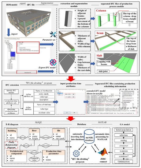
Figure 20.
The overflow of the automated optimization framework.
Finally, Table 6 reports the calculation results of the optimized project scheduling generated in the automated optimization framework. It reveals that if the team matrix is [1,2,1,10,1], the minimum completion time will be 13,106 min. If the team matrix is [1,2,3,10,1], the minimum completion time will be 7354 min. An improvement of 5752 min is therefore achieved with the proposed optimization method.
Table 6.
Solution results after adjustment and optimization.
6. Conclusions
With the ever-increasing availability of data and higher levels of automation and simulation, production scheduling in prefabrication factories can no longer be considered as an autonomous solution. Concepts such as BIM, graphic techniques, databases, and interface development, as well as a heightened emphasis on overall process optimization topics, have increased the pressure to connect to and interact with interrelated tasks and procedures. Considering the prefabricated element production, the ultimate objective of automation is to improve productivity, quality, and safety, which will also contribute to production schedule design. The automated optimization framework detailed in this study intended to generate optimal schedules for prefabricated component production based on the manufacturing process model and the GA method. In the case study investigated in this work, the automated optimization framework was proposed to improve the operability and accuracy of the production process model, which is generated by directly segmenting the IFC model. Moreover, the production time parameter is described by the properties in an extended IFC data schema, and the GA method is used to calculate the optimal alternative with parameters representing the geometric dimensions, production sequence, and time consumption. Based on the described integration technique, the data transmission and integration in the mating application program are achieved by linking a Python-based application, the MySQL database, and the computational environment. The implementation of the automated optimization framework for the production scheduling of prefabricated elements enables BIM models to play better foundational roles to fill the technical gaps between prefabricated building designers and element producers.
One of the conclusions that can be derived from this research is that more efforts are required to provide parametric descriptions of the production process of prefabricated elements in a more standardized way to facilitate their integration and automated processing via mating application programs. Database technologies and evolutionary computation techniques, such as the GA model, applied in combination with the IFC standard seem to be a possible path to improve the interoperability between BIM models and production scheduling tasks. This interoperability is also necessary to facilitate the reuse of the property sets of prefabricated elements provided in an extended IFC data schema, which are interlinked with other information outside BIM.
Some problems still exist, and they could be improved in the future. Firstly, the proposed implementation of prefabricated component segmentation based on IFC physical files was only designed for three typical components, namely columns, beams, and slabs. Additionally, the Python-based IFC file editing program developed in this research only functions with rectangular columns and rectangular beams according to designed segmentation rules. Future research work should contribute to expanding the capability to operate abnormal components by integrating new segmentation rules applied in prefabrication factories. This will introduce upgraded interfaces so that element producers can assign multi-task schedules for prefabricated component production. Furthermore, the addition of production time consumption parameters in the IFC model could enable the creation of new services to better support the communication between BIM designers and producers.
Author Contributions
Conceptualization, Z.X.; methodology, Z.X., X.W.; software, Z.X., Z.R.; writing—original draft preparation, Z.R., X.W.; writing—review and editing Z.X., X.W. supervision, Z.X.; funding acquisition, Z.X. All authors have read and agreed to the published version of the manuscript.
Funding
This research was funded by National Natural Science Foundation of China (72071043), the Ministry of Education of Humanities and Social Science project in China (20YJAZH114) and Natural Science Foundation of Jiangsu Province (BK20201280).
Acknowledgments
The authors’ special thanks go to all survey participants and reviewers of the paper, and appreciation to National Natural Science Foundation of China (72071043), the Ministry of Education of Humanities and Social Science project in China (20YJAZH114) and Natural Science Foundation of Jiangsu Province (BK20201280).
Conflicts of Interest
The authors declare no conflict of interest.
References
- Lu, W.; Chen, K.; Xue, F.; Pan, W. Searching for an optimal level of prefabrication in construction: An analytical framework. J. Clean. Prod. 2018, 201, 236–245. [Google Scholar] [CrossRef]
- Chen, J.H.; Hsu, S.C.; Chen, C.L.; Tai, H.W.; Wu, T.H. Exploring the association rules of work activities for producing precast components. Automat. Constr. 2020, 111, 103059. [Google Scholar] [CrossRef]
- Li, C.Z.; Xu, X.X.; Shen, G.Q.; Fan, C.; Li, X.; Hong, J. A model for simulating schedule risks in prefabrication housing production: A case study of six-day cycle assembly activities in Hong Kong. J. Clean. Prod. 2018, 185, 366–381. [Google Scholar] [CrossRef]
- Li, X.; Shen, G.Q.; Wu, P.; Yue, T. Integrating Building Information Modeling and Prefabrication Housing Production. Automat. Constr. 2019, 100, 46–60. [Google Scholar] [CrossRef]
- Jang, S.; Lee, G. Process, productivity, and economic analyses of BIM–based multi-trade prefabrication-A case study. Automat. Constr. 2018, 89, 86–98. [Google Scholar] [CrossRef]
- Costa, G.; Mardrazo, L. Connecting building component catalogues with BIM models using semantic technologies: An application for precast concrete components. Automat. Constr. 2015, 57, 39–248. [Google Scholar] [CrossRef]
- Abanda, F.H.; Tah, J.H.M.; Cheung, F.K.T. BIM in off-site manufacturing for buildings. J. Build. Eng. 2017, 14, 89–102. [Google Scholar] [CrossRef]
- Shi, A.; Pablo, M.; Mohamed, A.H.; Rafiq, A. BIM-based decision support system for automated manufacturability check of wood frame assemblies. Automat. Constr. 2020, 111, 103065. [Google Scholar]
- Li, S.; Isele, J.; Bretthauer, G. Application of IFC Product Data Model in Computer-Integrated Building Prefabrication. In Proceedings of the IEEE International Conference on Automation Science and Engineering, Scottsdale, AZ, USA, 22–25 September 2007; pp. 992–996. [Google Scholar]
- Jeong, Y.S.; Eastman, C.M.; Sacks, R.; Kaner, I. Benchmark tests for BIM data exchanges of precast concrete. Automat. Constr. 2009, 18, 469–484. [Google Scholar] [CrossRef]
- Lu, Y.; Xu, X.; Wang, L. Smart manufacturing process and system automation-A critical review of the standards and envisioned scenarios. J. Manuf. Syst. 2020, 56, 312–325. [Google Scholar] [CrossRef]
- Solihin, W.; Eastman, C.; Lee, Y.C. Multiple representation approach to achieve high-performance spatial queries of 3D BIM data using a relational database. Automat. Constr. 2017, 81, 369–388. [Google Scholar] [CrossRef]
- Zou, D.; Chen, K.; Kong, X.; Yu, X. An approach integrating BIM, octree and FEM-SBFEM for highly efficient modeling and seismic damage analysis of building structures. Eng. Anal. Bound. Elem. 2019, 104, 332–346. [Google Scholar] [CrossRef]
- Yin, X.; Liu, H.; Chen, Y.; Hussein, M.A. Building information modelling for off-site construction: Review and future directions. Automat. Constr. 2019, 101, 72–91. [Google Scholar] [CrossRef]
- Li, J.Q.; Yun, Q.H.; Duan, P.Y.; Han, Y.Y.; Niu, B.; Li, C.D.; Zheng, Z.X.; Liu, Y.P. Meta-heuristic algorithm for solving vehicle routing problems with time windows and synchronized visit constraints in prefabricated systems. J. Clean. Prod. 2020, 250, 119464. [Google Scholar] [CrossRef]
- Kim, T.; Kim, Y.; Cho, H. Dynamic production scheduling model under due date uncertainty in precast concrete construction. J. Clean. Prod. 2020, 257, 120527. [Google Scholar] [CrossRef]
- Ko, C.; Wang, S. Precast production scheduling using multi-objective genetic algorithms. Expert Syst. Appl. 2011, 38, 8293–8302. [Google Scholar] [CrossRef]
- Wang, Z.; Hu, H.; Gong, J.; Ma, X. Synchronizing production scheduling with resources allocation for precast components in a multi-agent system environment. J. Manuf. Syst. 2018, 49, 131–142. [Google Scholar] [CrossRef]
- Leu, S.; Hwang, S. GA-based resource-constrained flow-shop scheduling model for mixed precast production. Automat. Constr. 2002, 11, 439–452. [Google Scholar] [CrossRef]
- Anvari, B.; Angeloudis, P.; Ochieng, W. A multi-objective GA-based optimization for holistic Manufacturing, transportation and Assembly of precast construction. Automat. Constr. 2016, 71, 226–241. [Google Scholar] [CrossRef]
- Wang, Z.; Hu, H.; Gong, J. Framework for modeling operational uncertainty to optimize offsite production scheduling of precast components. Automat. Constr. 2018, 86, 69–80. [Google Scholar] [CrossRef]
- Shi, X.; Liu, Y.S.; Gao, G.; Gu, M.; Li, H.J. Ifcdiff: A content-based automatic comparison approach for ifc files. Automat. Constr. 2018, 86, 53–68. [Google Scholar] [CrossRef]
- Chen, P.H.; Cui, L.; Wan, C.; Yang, Q.; Ting, S.K.; Tiong, R.L.K. Implementation of IFC-based web server for collaborative building design between architects and structural engineers. Automat. Constr. 2005, 14, 115–128. [Google Scholar] [CrossRef]
- Nepal, M.P.; Staub-French, S.; Zhang, J.; Lawrence, M.; Pottinger, R. Deriving construction features from an IFC model. Proceedings, Annual Conference—Canadian Society for Civil Engineering; INC.: Quebec City, QC, Canada, 2008; pp. 426–436. [Google Scholar]
- Khalili, A.; Chua, D.K.H. IFC-based framework to move beyond individual building elements toward configuring a higher level of prefabrication. J. Comput. Civil Eng. 2013, 27, 243–253. [Google Scholar] [CrossRef]
- Zhang, L.; Issa, R.R.A. Ontology-Based Partial Building Information Model Extraction. J. Comput. Civil Eng. 2013, 27, 576–584. [Google Scholar] [CrossRef]
- Baldacci, F.; Desbarats, P. Parallel 3D Split and Merge Segmentation with Oriented Boundary Graph. In Proceedings of the 16th International Conference in Central Europe on Computer Graphics, Visualization and Computer Vision, Plzen-Bory, Czech Republic, 4–7 February 2008. [Google Scholar]
- Zhu, J.X.; Wang, X.Y.; Wang, P.; Wu, Z.Y.; Kim, M.J. Integration of BIM and GIS: Integration of BIM and GIS: Geometry from IFC to shapefile using open-source technology. Automat. Constr. 2019, 102, 105–119. [Google Scholar] [CrossRef]
- Marras, I.; Nikolaidis, N.; Pitas, I. 3D geometric split-merge segmentation of brain MRI datasets. Comput. Biol. Med. 2014, 48, 119–132. [Google Scholar] [CrossRef]


Publisher’s Note: MDPI stays neutral with regard to jurisdictional claims in published maps and institutional affiliations. |
© 2020 by the authors. Licensee MDPI, Basel, Switzerland. This article is an open access article distributed under the terms and conditions of the Creative Commons Attribution (CC BY) license (http://creativecommons.org/licenses/by/4.0/).