1. Introduction
In the preparation of baking goods, dough fermentation is one of the most important steps. Although fermentations of doughs have been applied for several thousand years, online measurement systems for important process variables are still rare [
1]. During this process step, the basis for the later structure of the pore system of the final product is set. The bubbles introduced during the kneading will increase in volume, due to the diffusion of CO
2, which is produced by the yeast cells. The dough fermentation process depends on the quality and amount of yeast cells added during mixing, the dough stability, the flour quality, the ingredients, and the dough yield as well as the fermentation conditions (temperature, humidity, air flow, and fermentation time) [
2,
3,
4].
For the supervision of the dough fermentation process, several approaches have been developed. Cuenca et al. [
5] applied isothermal micro-calorimetry to monitor food fermentation processes. Analyzing the maximum heat flow, the time to reach the maximum heat flow, and the enthalpy, they could demonstrate that the flour mixtures had a strong influence on all these values. Thus, a characterization of the process based on micro-calorimetry seems possible. Moreover, different optical systems were developed. Chevallier et al. [
6] measured the expansion of bread dough during fermentation. Three methods for image acquisition with a digital camera were used: vertical expansion of the dough in a flask, horizontal expansion between two plates, and free expansion. The evaluation of the measurements based on the Gompertz function showed that the proving temperature had a significant effect on the different function parameters calculated (volume expansion ratio, expansion rate), while the water content had no significant effect. Zettel et al. [
7] described a camera system that was able to determine the volume of dough pieces in a proofing chamber. Based on a mathematical model by Stanke et al. [
8], it was possible to predict the volume change over time based on measurements obtained after 300, 600, and 3000 s of fermentation. The mean percentage difference of measured and overall simulated values (including fit and forecast) was 2.1%, 1.3%, and 0.8% for the fit after 300, 600, and 3000 s, respectively. Based on an image analysis system, Yousefi-Darani et al. [
9] determined the relative volume increase of dough pieces in a proofing chamber and used this for a PID (proportional integral derivative) closed-loop control system. They demonstrated the controller performance by using different amounts of yeast as well as different starting temperatures of the dough pieces (normal state, frozen state, and thawed state). Comparing PID control with a fuzzy control system, Yousefi-Darani et al. [
10] showed that similar results of both control algorithms were obtained, but that the fuzzy controller was much faster to implement. Ivorra et al. [
11] developed a 3D vision system for the monitoring of dough fermentation; using a laser and a camera system combined using the structured light technique, they obtained a 3D sample profile during fermentation. Differences in dough behaviors during fermentation were found based on the structured light method. They related the variation of the total transversal area to the maximum height at each fermentation time and obtained a set of peaks and valleys. The number of peaks can be used to obtain information about the fermentation capacity of the samples. In a further study by that research team, Verdú et al. [
12] obtained information about the internal structure of bread dough during the fermentation process using their 3D vision system as well as 2D images of baked dough samples. They observed correlations between the 3D and 2D information, specifically between the transversal area and height (3D) and final bubble size and number of bubbles (2D). A similar approach was presented by Giefer et al. [
13], who applied a movable laser sensor system that was located at the back of the fermentation chamber and complemented it with a superellipsoid model fitting method. They showed that the volume of each object could be estimated with a deviation of approximately 10% on average.
To reduce the errors in measurements and to estimate non-measurable process variables, a Kalman filter can be applied. Although there are several applications of the Kalman filter for fermentation processes [
14,
15,
16,
17,
18,
19,
20], its application is still rare in the food area. Recently, Pongsuttiyakorn et al. [
21] used weight sensors, which are inherently contaminated by noise, and complemented them with a Kalman filter to correct the real-time measured weight under various temperatures to determine the moisture content during the food drying process. They showed the effectiveness of their approach using pineapples as the food material. Azimi et al. [
22] applied a special version of an extended Kalman filter for the produce wash system of lettuce. To obtain the best possible estimation performance, they used a particle swarm optimization algorithm to optimize offline the covariance matrices of the process noise. This matrix was then used by the Kalman filter in real-time to estimate the chemical oxygen demand in the wash water, the free chlorine concentration, the
E. coli concentration in the wash water, as well as the
E. coli level on the lettuce. Applying a sensitivity analysis, the authors demonstrated that the estimator had good robustness. To decontaminate the surfaces of potatoes, Ulloa et al. [
23] applied a Luenberger observer, which is similar to a Kalman filter. Based on temperature and weight loss data, the developed observer was able to estimate the internal food temperatures. This is important to prevent thermal food damages such as cracking. Abdel-Jabbar et al. [
24] applied a linear state space dynamic model to describe drying in continuous fluidized bed dryers. They used a Kalman filter to provide state estimates for an optimal state feedback control system and obtained acceptable performance even when starting with incorrect initial states. For a fuzzy control system for the gari (i.e., one of the most popular foods produced from cassava) fermentation plant, Odetunji and Kehinde [
25] applied an algorithm based on the Kalman filter for calculating the parameters of a linear algebraic equation that yields the least squares of errors.
In the present study, a continuous-discrete extended Kalman filter was applied to monitor and estimate important variables of a dough fermentation process over time. As the measurement system, an image analysis system was used to determine the total dough volume and radius of an average bubble inside of the fermentation good. The discrete measurements were complemented with a nonlinear dynamic mathematical dough model, based on the Bernoulli equation, the CO2 production by yeast cells, and diffusion processes. Using the extended Kalman filter, estimates of the bubble radius, the amount of CO2 molecules in a bubble, the CO2 concentration in the non-gas dough, and the production rate of CO2 were estimated online.
2. Materials and Methods
A detailed description of the Kalman filter can be found in the literature [
26].
2.1. Dynamic Mathematical Model for Dough Fermentation
The model used in this investigation was described in detail by Stanke at al. [
8]. The following assumptions were made for the modelling: during kneading, only nitrogen is introduced into the dough (because we assumed just anaerobic consumption of the sugars), no CO
2 and no new bubbles are formed during fermentation, a pure Newtonian behavior of the dough is assumed so the Bernoulli equation can be used complemented by the continuity equation. Moreover, we assumed that the bubbles are spherical and homogeneously distributed throughout the dough, all bubbles have the same radius, the yeast and therefore the CO
2 production is homogeneously distributed over the dough, growth of yeast is not considered, only CO
2 diffusion is considered, no coalescence and disproportionation are considered, all the gas is retained in the dough, and the ideal gas law can be applied.
Therefore, for the extended Kalman filter, the following equations are obtained:
where
r is radius of all bubbles, t is the time,
n is the amount of CO
2 in mol in a single bubble,
if the CO
2 concentration in non-gaseous dough,
is the specific CO
2 production rate,
RG is the gas constant,
T is the temperature,
is the viscosity,
pD is the pressure in the dough,
. is the surface tension,
. is the yeast concentration,
D is the diffusion coefficient of CO
2,
H is the Henry constant for CO
2 and water,
r0 is the radius at
t = 0 s, and
zi(
t) represents the non-correlated process error noise, whose expectation value is zero.
The last differential equation was introduced to estimate the specific CO2 production rate by the extended Kalman filter. Obviously, during the simulation no change will occur; however, during filtering, the values of the CO2 production will be adapted to the actual value.
2.2. Image Acquisition System
The dough pieces were placed in front of a camera (DFK 31BU03.H, Image Source Europe GmbH, Germany) with a resolution of 1024 × 768 pixel. They were positioned on a black baking pad to avoid reflections from light and to improve the border detection for the automated object acquisition. A picture was taken every three seconds and evaluated via a border detection script using MATLAB 2019a (version 9.6.0). The imaging evaluation software provides the radius of an average bubble assuming a fixed number of bubbles as N
B and a start radius of the bubbles as
r(
t = 0). Their values are presented below. Therefore, as the only measurement for the extended Kalman filter, the radius of an average bubble was used in the following equation:
Every 3 s, a measurement was sent to the extended Kalman filter. To verify the volume measurement obtained by the image analysis system, the results were compared with those determined by a volume laser scanning system (Volscan profiler 600, Stable Micro Systems, Winopal Forschungsbedarf GmbH, Elze, Germany).
2.3. Software Implementation
The image analysis software as well as the extended Kalman filter were developed using the software Matlab® 2019a (version 9.6.0) and the “Symbolic Math” toolbox (version 8.3). The latter was used to calculate the estimation error covariance differential equation matrix (16 equations). For all calculations, a normal office PC (Intel Core® i5 8500 with 8 GiB of RAM) with Windows 10 was used. For the simulation, a system of 20 (4 + 16) differential equations in total was solved numerically using the ode45 method from Matlab®, which is based on an explicit Runge-Kutta formula.
2.4. Preparation of Dough
The doughs were prepared with commercial wheat flour (200 g, Schapfenmühle, type 550: 0.51–0.63% mineral supplements in dry matter, corrected to the moisture content), water (119.18 g), salt (4 g), and commercial yeast (2 g, Omas Ur Hefe, Fala, Germany) in a mixer (N50, Hobart GmbH, Germany). Mixing time and water temperature were kept constant at 4 min and 32 °C, respectively, and the temperature of the prepared dough ranged between 23.8 and 27.8 °C depending on the room temperature. After the preparation, hand-rounded 50 g dough balls were set in a proving cabinet (Klimaschrank VC 4033, Vötsch Industrietechnik GmbH, Germany) for 40 min at 30 °C and 80% humidity.
2.5. Parameters of the Models and the Extended Kalman Filter
The parameters used in the mathematical dough model and the extended Kalman filter are presented in
Table 1. The amount of nitrogen in a bubble was calculated using the ideal gas law and the start radius of the representative bubble. Most of the values were taken from the literature. The diagonal values of the process noise spectral matrix Q
ii were determined during simulations. A measurement error was assumed that was more than half of the radius
r(
t = 0); therefore, the measurement noise variance R was fixed at 10
−9 m². The initial conditions for the numerical solving of the differential equations for the mathematical dough model and the estimation error covariances are presented in
Table 2. The values of Q were obtained by performing experiments.
3. Results
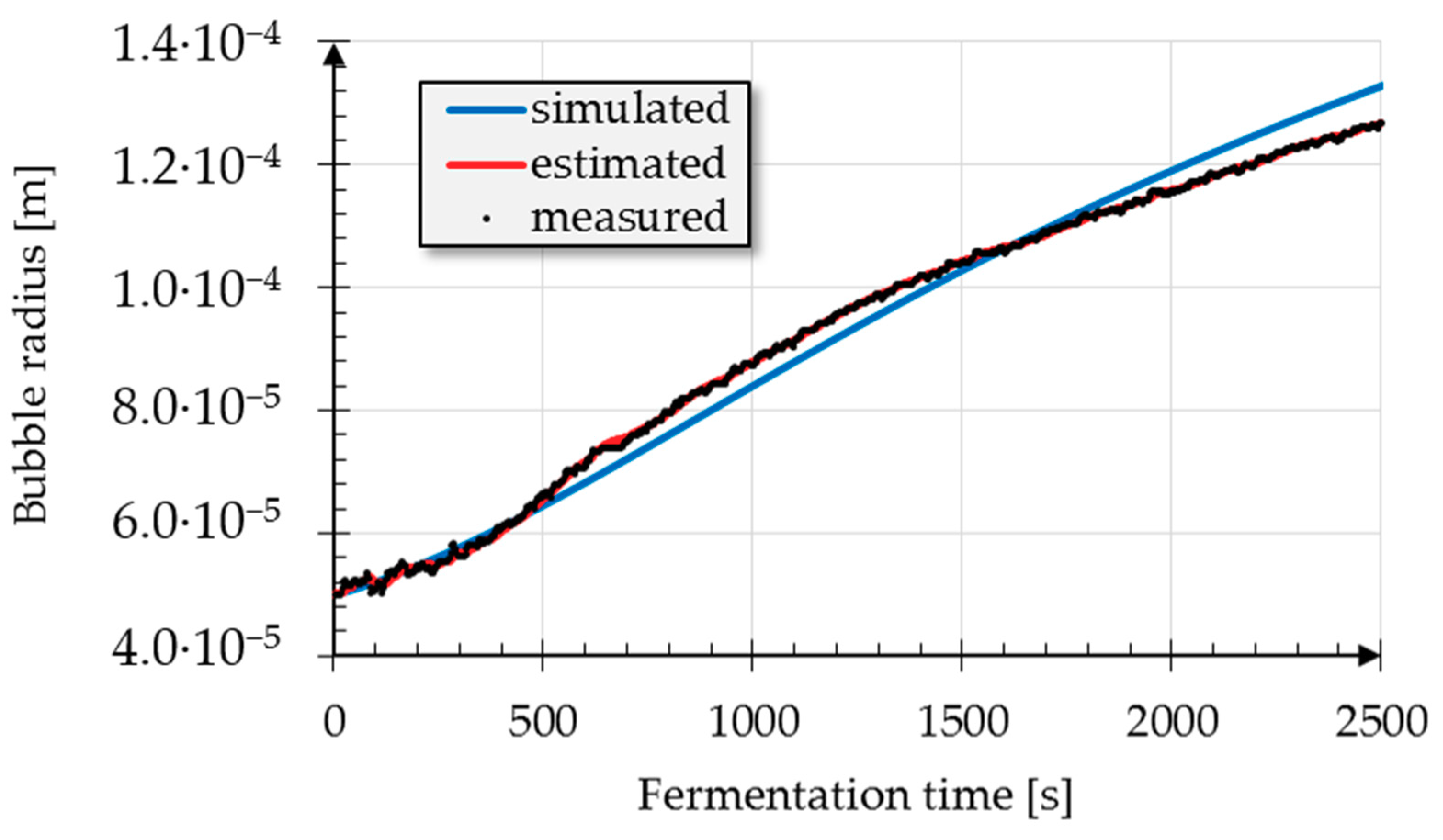
Figure 1 presents the online measurements of the bubble radius (see
Table S1, Supplementary Material), its estimated values, as well as the purely simulated values using just the initial conditions. When a deviation of the measured and estimated values was present, the estimated values tended towards the measured ones, indicating that the mathematical dough model was not dominating the estimation. At around 645 s fermentation time, the imaging system presented the same radius several times, and as a consequence, the estimated radius were increasing more slowly. Overall, there were 423 measurements below and 418 measurements above the estimated values, indicating that there was no systematic deviation due to the estimation. During the fermentation, the radius more than doubled its value, which shows that the gas volume increased by more than eight fold. Considering a start volume of 10 % of the total dough volume, then the final dough volume was 2.4 times its start value. The purely simulated values were in between 500 and 1500 s below the estimated and after 1700 s above them. This indicated that the cells produced more CO
2 during the first time period and less at the end. A difference of 7 µm between the simulated and estimated radius was present at the end of fermentation. The overall simulated and estimated values followed roughly the same line, indicating that the values of R and Q might be balanced. If only the values of the radius are considered, the advantage of the extended Kalman filter is not immediately obvious.
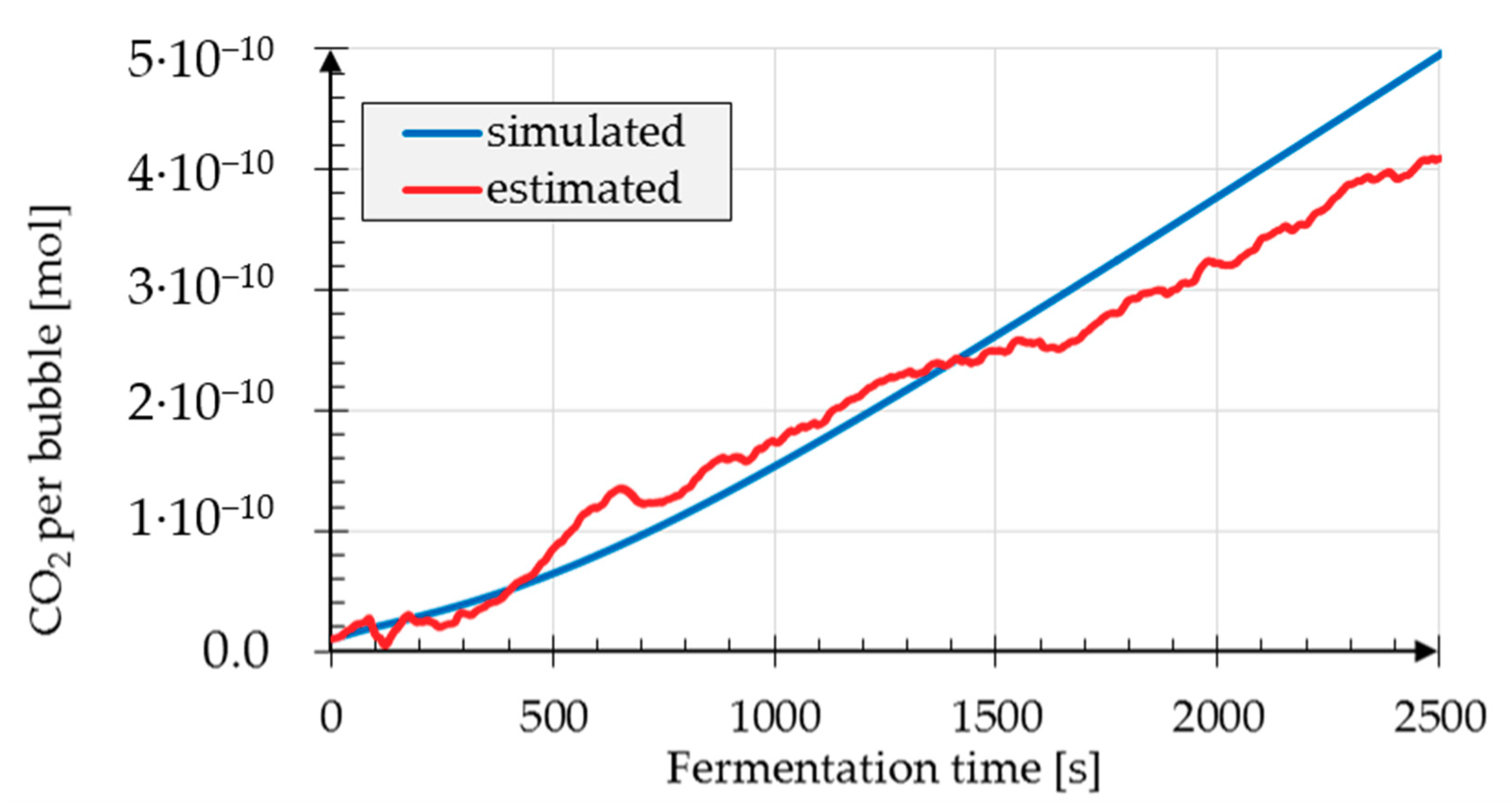
However, further information was obtained, as shown in
Figure 2, where the CO
2 amount in the representative bubble is presented as estimated and simulated. Here, a similar behavior can be recognized. However, the estimated values were higher here from slightly before 500 s to 1400 s and always lower after 1500 s. At 645 s, the increase of the CO
2 values reduces significantly. This is the consequence of the constant values of the radius measurements. At the end of the fermentation, a difference of almost 10
−10 mol can be seen, indicating that the cells might have had less amount of substrate available, which can be due to less damaged starch due to lower enzyme activity converting amylose and amylopectin to fermentable sugars. The different evolution of the simulated and estimated values was more pronounced around 100 s, as seen in
Figure 3.
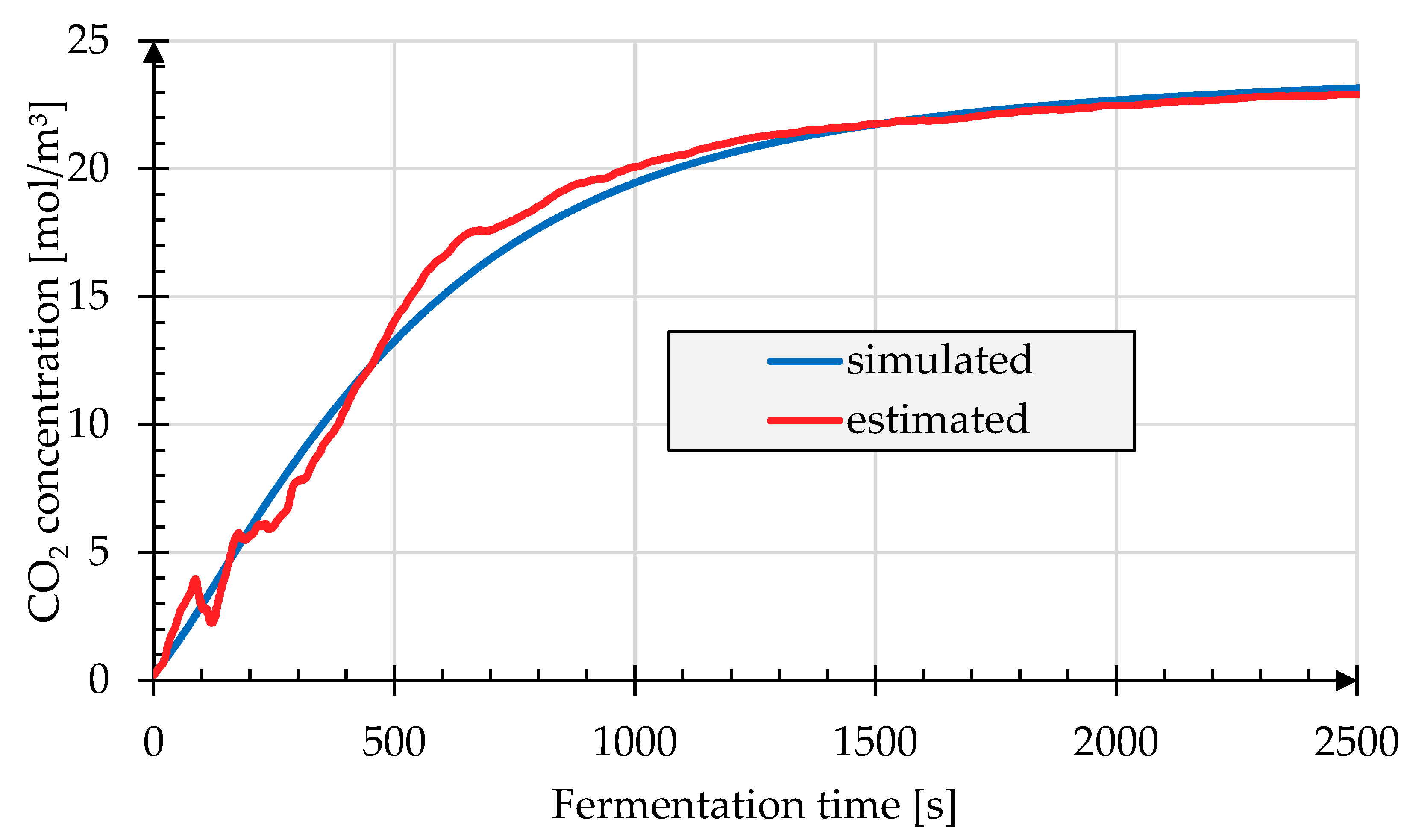
In
Figure 3, the simulated and estimated values of the CO
2 concentration in the non-gaseous dough phase are presented. After a steep linear increase at the beginning of fermentation, a saturation seems to be reached at the end. Roughly before 100 s, the estimated values decrease significantly, which is due to the fact that the measurements of the radius decrease, which seems to be an error of the image evaluation system. The measurements of the radius are smaller than the estimated radius. To compensate that, the CO
2 in the non-gas phase as well as the amount of CO
2 in the representative bubble were almost constant until the radius increased again. However, after that fermentation time, the values of the CO
2 in the non-gaseous dough phase converged slowly to the saturation value. However, the amount of CO
2 in a bubble still increased almost linearly.
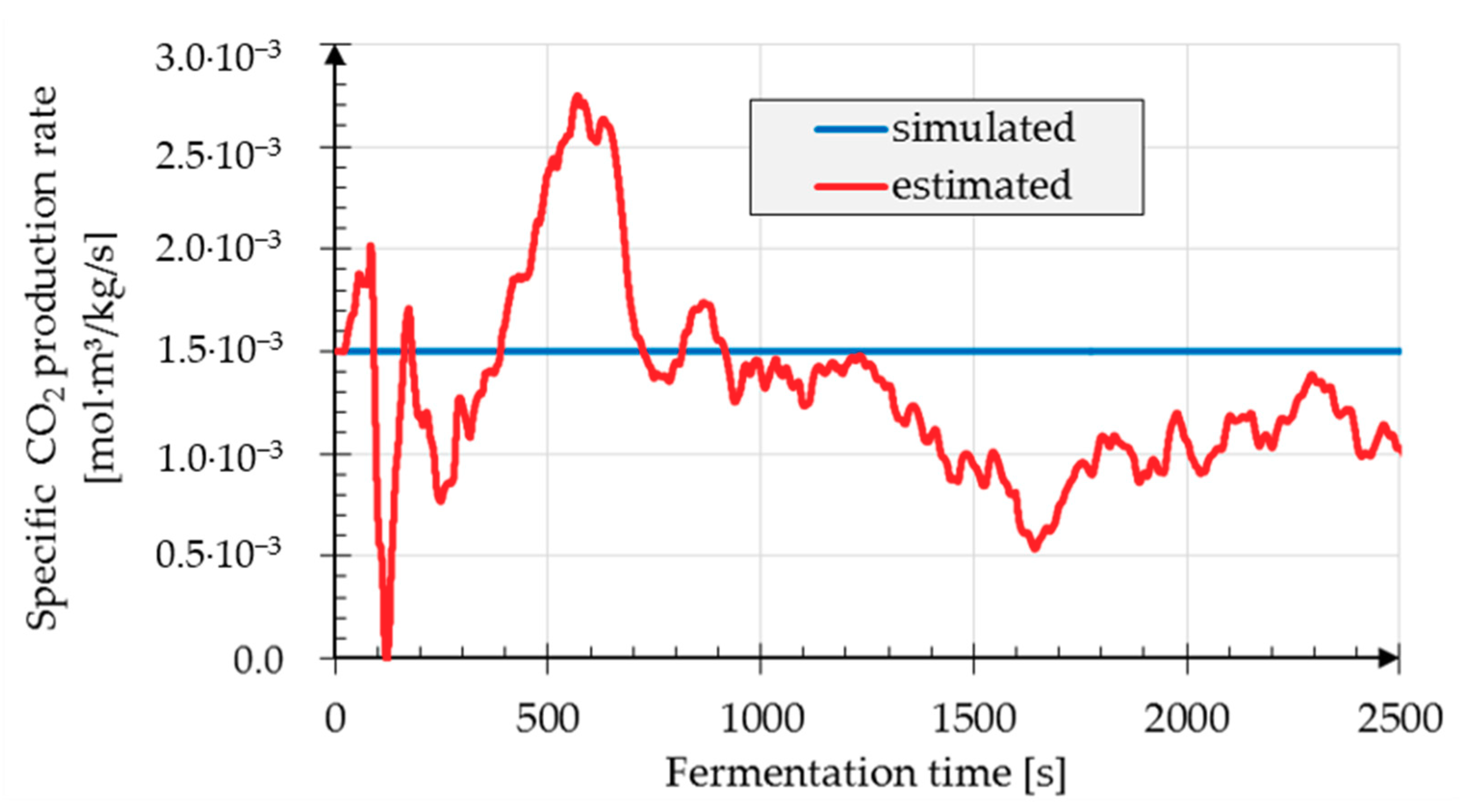
The values of the specific CO
2 production rate fluctuated even more, as one can see in
Figure 4. At the beginning, an up and down trend can be observed, which is due to the increased and decreased radius measurements around 100 s fermentation time. After 250 s, a steep increase in the CO
2 production rate to almost the double value can be seen. After 645 s fermentation time, the production rate decreased to levels under the start value, the lowest value being reached at 1650 s fermentation time. The increase at the beginning might be due to the increase in temperature, which was higher in the fermentation chamber than during the dough preparation. The decrease might be a result of the limiting substrate concentration, as only damaged starch can be converted to fermentable sugars. The fermentation lasted more than 40 min, so most probably the cell number increased due to growth. However, this was not considered in the model (X is constant). If the cell count increased in reality but not in the model, then the filter could compensate for this fact by an increase in the specific CO
2 production rate, which might explain the moderate increase during the last 800 s.
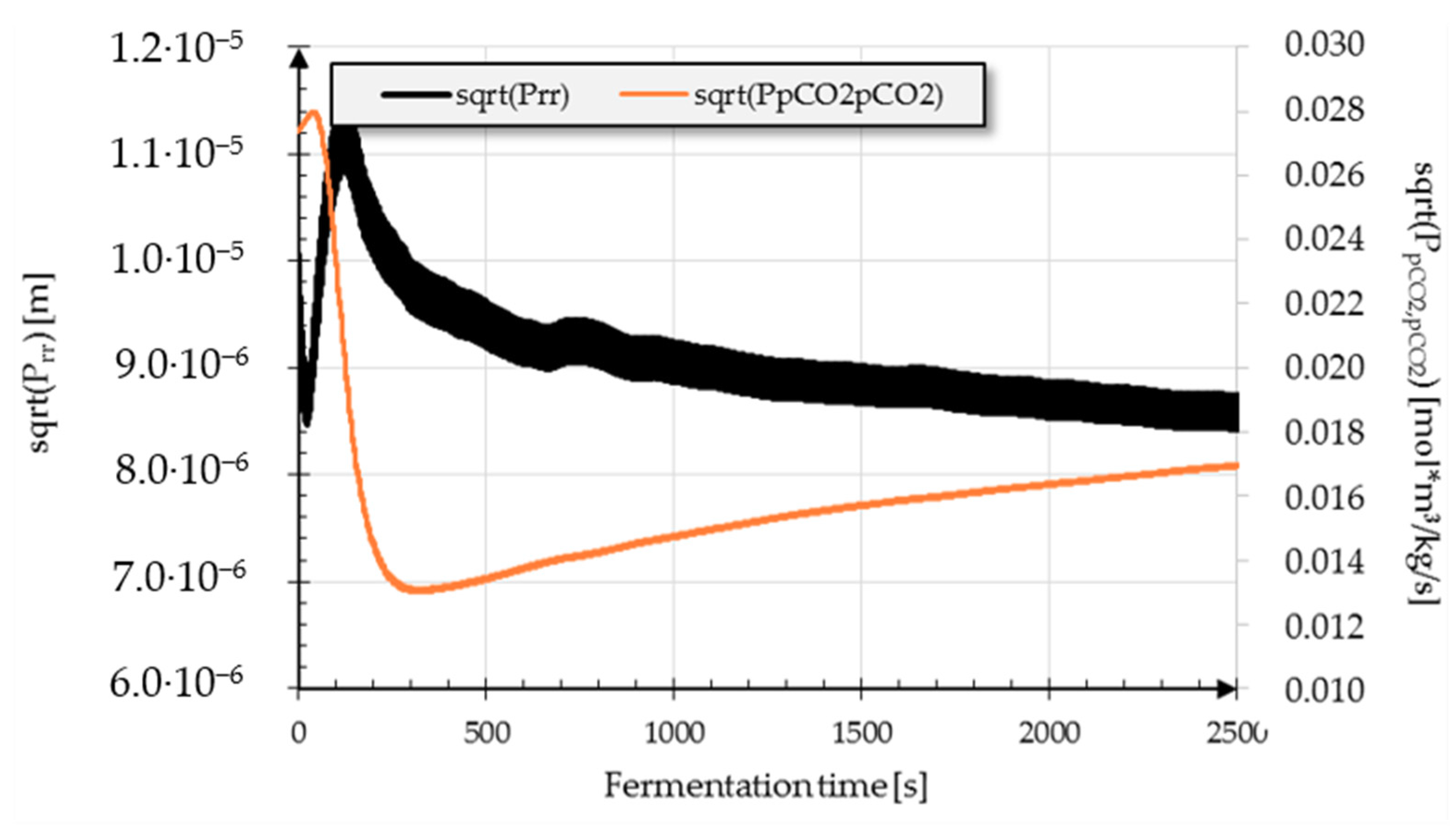
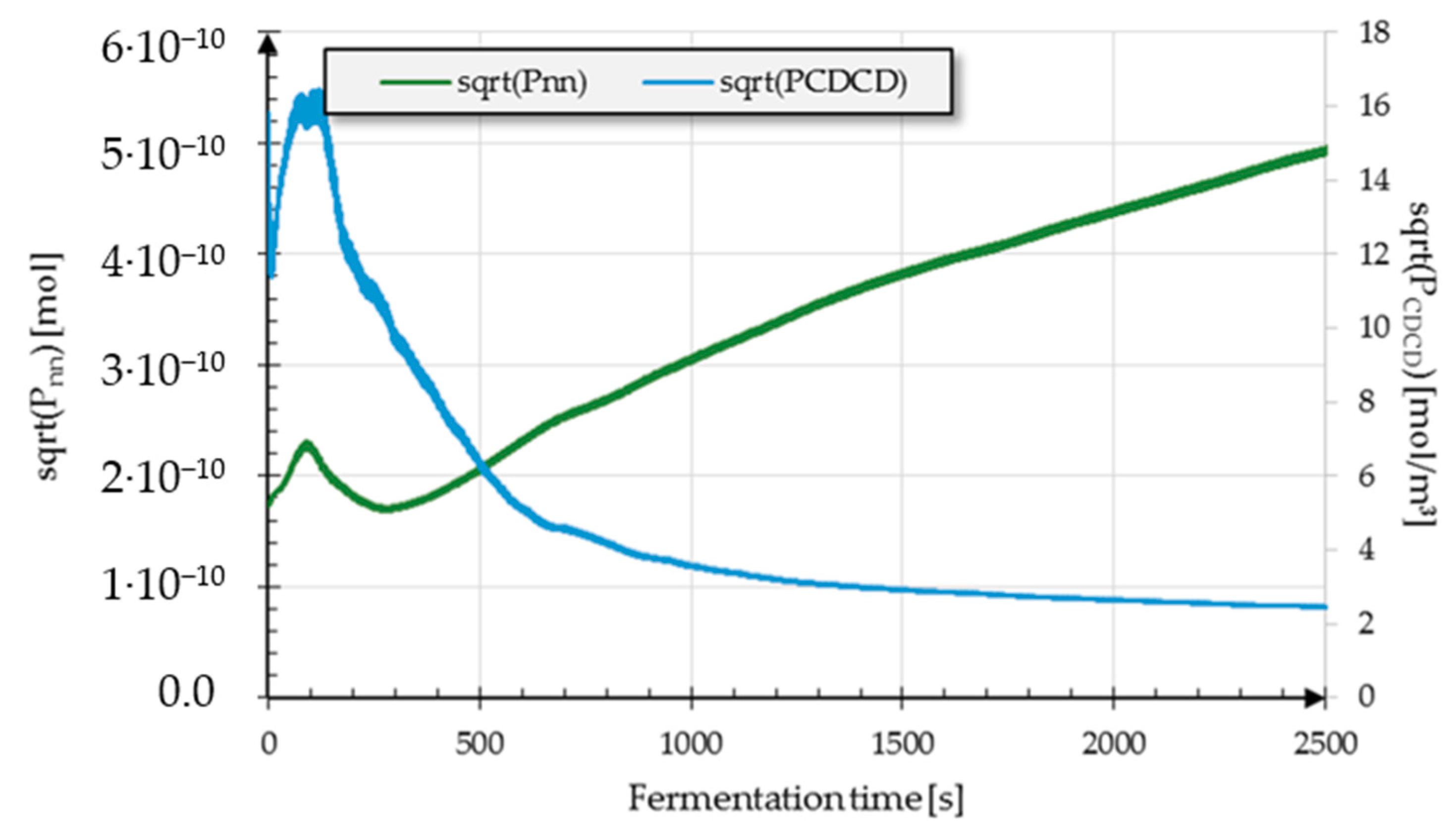
Further information obtained by the extended Kalman filter algorithm can be seen in
Figure 5 and
Figure 6, where the square root of the estimation error variances of the radius, the specific CO
2 production rate, the CO
2 in non-gas dough, and the CO
2 amount in the bubble can be seen. For the radius, after a short decrease, the values jumped up to 1.15 × 10
−5 m, due to the difference between the measured and estimated values for the radius, and then decreased slowly to 8.5 × 10
−6 m with a fast up and down trend every 3 s. The values increased when no measurement was present and decreased rapidly during the filtering, when a measurement was obtained; therefore, the line appears thick. This was also true for the other estimated variables but with a much smaller amplitude. The estimation error of the specific CO
2 production rate presented a steep decrease to 0.014 mol·m³/kg/s during the first 300 s fermentation time, followed by a gentle increase to 0.016 mol·m³/kg/s at the end of fermentation.
The estimation error of the amount of CO2 in the representative bubble, with an exception at the beginning, increased almost linearly. The values for CO2 in the non-gas phase jumped at the beginning to 16 mol/m³ and after a while decreased almost exponentially to roughly 2 mol/m³. The reason for the decrease might be that the values approach the saturation level.
If the square roots of the median values of the estimation error variances are divided by the median of the corresponding process variables, the following values are obtained: 0.09 for the radius, 0.15 for the CO2 in the non-gaseous dough, 1.5 for the amount of CO2 in the bubble, and 13 for the specific CO2 production rate. Therefore, the specific CO2 production rate had the highest relative estimation error, and the error was much higher than the values themselves. The values of the amount of CO2 in the bubble had an error of same order of magnitude as the corresponding CO2 values. The estimation errors of the radius and the CO2 in the non-gaseous dough phase were one order of magnitude smaller than the values of the corresponding process variables.
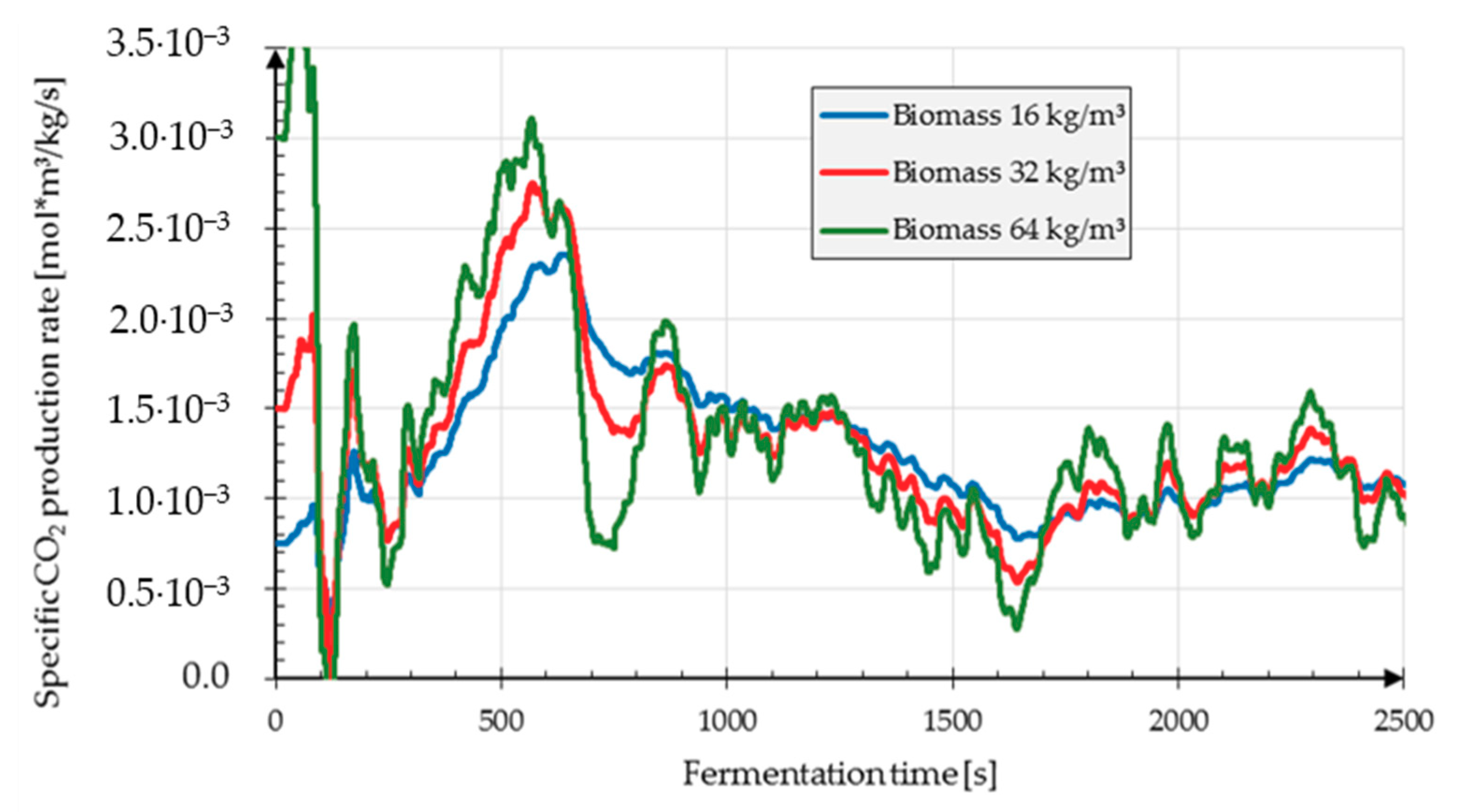
To prove the capability of the extended Kalman filter for the estimation of the specific CO
2 production rate, two new runs of the extended Kalman filter were carried out changing the biomass concentration X. The yeast cell mass in the model was changed to analyze the estimation performance of the extended Kalman filter.
Figure 7 shows the specific CO
2 production rate in three different runs of the extended Kalman filter using the same measurements: one run where the biomass concentration was correctly specified (X = 32 kg/m³), one with half of the value (X = 16 kg/m³), and one with twice as much (X = 64 kg/m³). To compare the values more easily, the production rate was divided or multiplied by 2 where half or twice as much yeast concentration was assumed, respectively. For the production rate of half the yeast concentration, it took more than 800 s for the filter until the correct value was obtained. This was much faster when twice the yeast concentration was assumed. Here, after 250 s the correct value was reached. The pattern of the correct values and the one obtained with twice the yeast concentration were almost the same, although sometimes the values were smaller, sometimes higher; but the same up and down trend was clearly followed. This indicates that the values themselves might be better than the estimation error variance suggests.
Although some of the estimation errors were high, the information obtained with the extended Kalman filter for the supervision of dough fermentation was significant. More information was obtained beyond the volume of dough pieces.


