Abstract
Modeling and optimization of a double-inlet pulse tube refrigerator (DIPTR) is very difficult due to its geometry and nature. The objective of this paper was to optimize-DIPTR through experiments with the cold heat exchanger (CHX) along the comparison of cooling load with experimental data using different boundary conditions. To predict its performance, a detailed two-dimensional DIPTR model was developed. A double-drop pulse pipe cooler was used for solving continuity, dynamic and power calculations. External conditions for applicable boundaries include sinusoidal pressure from an end of the tube from a user-defined function and constant temperature or limitations of thermal flux within the outer walls of exchanger walls under colder conditions. The results of the system’s cooling behavior were reported, along with the connection between the mass flow rates, heat distribution along pulse tube and cold-end pressure, the cooler load’s wall temp profile and cooler loads with varied boundary conditions i.e. opening of 20% double-inlet and 40-60% orifice valves, respectively. Different loading conditions of 1 and 5 W were applied on the CHX. At 150 K temperature of the cold-end heat exchanger, a maximum load of 3.7 W was achieved. The results also reveal a strong correlation between computational fluid dynamics modeling results and experimental results of the DIPTR.
1. Introduction
The pulse tube cooler was a technology that evolved with a series of developments primarily in the beginning of the 1980s. Each cryocooler is simple to operate and has high reliability, as compared to other cryocoolers. The main benefit was the absence of moveable components in the region with low temperatures, leading to less mechanical vibrations that are suitable for a wide range of applications. In the first instance, for several industrial applications, such as gas separation and liquefaction, the new type of pulsing tube refrigerator with a low-temperature valve was introduced. However, due to its geometrical behavior, it was difficult to run a simulation on it using limited resources. One of the best differentiating techniques of the double-inlet pulse tube refrigerator (DIPTR) simulation is the finite volume method (FVM) to obtain these factors. This FVM approach addresses legislative equations for liquid mass flow, heat exchange and problems with fluid diffusion, and the results are consistent with the formulas for preserving weight, momentum and energy [1]. A basic pulse tube refrigerator (PTR) was originally invented [2]. The impact of multidimensional streams on a high-frequency inert pulse pipe was also investigated [3]. A single-stage pulse tube refrigerator (SSPTR) numeric model was made for adiabatic flow. The pressure oscillations of compressor, PT and reservoir were derived with the assumption that compressor volume varies sinusoidally, and this gives a reasonably good agreement between the theoretical and experimental data. The influence of factors like hydraulic diameters, length, temperature resistance and permeability factor on the cooling behavior and performance was examined [4]. The thermodynamic process of gas parcels within the regenerator as well as flow and heat transfer for 50 Hz PTR operations was investigated as a model based on Lagrangian illustration. The SIMPLER algorithm solves the control equations and Darcy–Brinkman–Forchheimer was used as a porous model [5]. The acoustic power generated by the thermoacoustic traveling-wave engines (TATWEs) can be used as a thermal-electric alternator. The cooling generation can be used to generate electricity using a thermoacoustic cooler or PTR by changing the regeneration impedance and its length effects by system debugging [6]. Initial simple pulse tube refrigerator (IPTR) design was improved with the addition of an opening valve between pulse tube and reservoir, enhancing IPTR’s performance significantly. This modification leads to the orifice pulse tube refrigerator (OPTR). A key step in developing a cooling pulse tube was the simple invention of OPTR [7]. In order to understand the operating mechanism of the three common types of pulse tube refrigerators, the analysis of the thermodynamic behavior of gas elements of pulse tube has been done and was taken as an adiabatic process [8]. At the time of contraction and extension, the stress variance within the pulse pipe was symmetrical. It was considered a trapezoidal variance of room for the accuracy of the equations. An OPTR studied an important flow and heat transfer processes for a cyclic moving piston at one end of the system—helium as the working fluid. The regenerator, like many heat exchangers, was mounted into a porous medium and was not thermal equilibrium configured. The output of the OPTR was improved by generating a dead region between the cold and warm edges of the pulses, resulting in a higher frequency of bi-cellular structure [9].
The regenerator and all heat exchangers have multiple devices in the case of viscous gas and inertial loss. The OPTR stirling CFD axisymmetric model for the simulation was used, as the regenerator and pulses was essentially identical and their physical characteristics for gases and solid materials remain unchanged [10]. The double-inlet orifice pulse tube control refrigerator (DIOPTR) connects the skirt directly to the outlet of the compressor and inlet of the reservoir, where the excess fluid is passed to the compressor and eliminates the reduction of the regenerator losses. A minimum temperature of almost 3.5 K was achieved with multi-stage pulse tube refrigerator [11]. The time-based CFD calculations for both inline and intermediate OPTR operation average was analyzed. Accordingly, theoretical and numerical refrigeration of pulse tube system was described with precise measurements of the temperature production and the flow zone predictions. [12].
The premise that a pulse tube refrigerator is called the stirling split refrigerator type and that a gas on the pulse tube is split into three parts was an isothermal approach to the development of pulse tube refrigerators [13]. In the smaller frequencies of the PTR stirling, the GM pulse tube cooler has distinct flux and heat transfer functions [14]. The phase and volume effects of the active phase controller on the phase, mass movement, pressure ratio and efficacy of the refrigerating pulse tube have also been studied using a two-dimensional axis-symmetric CFD computer analysis [15]. In 220 W-input theoretical electrical equipment, the configuration of the mesh segments used indicates how it was configured in order to achieve optimum cooling efficiency or the lowest exergy level, the non-load temperature of 27.2 K and the cooling energy [16]. A 1.22 kg coaxial miniature pulse tube cryocooler (MPTC) was developed and examined for cooling related to cryogenic applications requiring compactness, less weight and fast cooling rate. The regenerator, pulse tube and phase shifter geometrical parameters were optimized [17].
A DIPTR with a dual inlet valve connected to the pulse cooler was developed to improve the refrigeration effect [18]. Various software analyses and models have been developed in order to evaluate the cooling and loss processes [19,20]. Nevertheless, the exact nature of the physical phenomena that induce pulse tube coolers (PTR) activity was not well understood. Most of these solutions to date were based on a single-dimensioned flow, which was not enough to expose the features of multi-dimensional flow [21,22]. CFD software, such as Fluent, is a powerful tool for Navier–Stokes mathematical solutions that have a finite choice of volumes, and have shown that the pulse tube refrigerator (PTR) was subject to CFD simulations [23]. The pressure inlet limits for DIPTR simulation at constant temperatures or thermal flow limits was set at a single tube end, and at the external heat exchange and cold-end simulation [24]. The inertance-type pulse tube refrigerator ITPTR model was limited by the fact that, compared to the DIPTR mode, it cannot reach a much lower temperature [25]. The analysis of a GM cryocooler linear dynamic system was performed and a limited temperature range was considered in a setting [26]. The DIPTR was adjusted to the phase shift between the pressure wave and the mass flow in the pulse tube and to increase its amplitudes. The double-inlet resistance and the orifice resistance were optimally balanced [27,28]. A three-dimensional fluid and heat transfer system was used in the pulse tube and heat exchange (HE) pulse tube refrigerator (PTR) to detect the impact factor for the efficiency of a pulse tube cooler [29]. First-time computational fluid dynamics method with FLUENT CFD solution program was used to solve a single-phase iterance pulse tube refrigerator [30].
The aim was to use the FLUENT simulation in order to present the fundamental analysis of Gifford-McMahon-type double-inlet pulse tube refrigerator (GM-DIPTR) design and conform to the quantitative results with appropriate experimental data. In this present research, we conducted CFD analysis on a 2-D model of GM-type DIPTR using ANSYS by applying different load conditions with some initial boundary conditions. Additionally, we employed five different simulation cases with different boundary conditions and loads on it, while double-inlet valve percentages also varied gradually to achieve a best load. By applying this, a load of 3.7 W was obtained at a temperature of 155 K, as the initial temperature was gradually increased up this to achieve the best load. Then a comparison was made with previous experimental data and the current CFD results.
2. Materials and Methods
2.1. Geometry of GM-Type DIPTR
Figure 1 shows the 2-D modeled DIPTR, for which the geometry of Gifford-McMahon-type DIPTR was compared with literature [31]. The dimension of DIPTR was taken in L/D ratio, which was for transfer line 21.098, after cooler 0.846, regenerator 9.772, heat exchanger cold-end 1.470, pulse tube 16.8, heat exchanger hot-end 0.956 and for reservoir 2.772. In the C programming language, a user-defined function (UDF) for gas pressure and depressurization was built in the closed chamber.
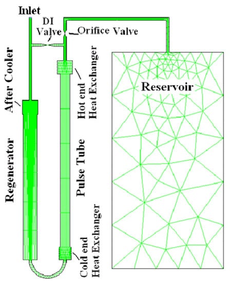
Figure 1.
Geometry of GM-type double-inlet pulse tube refrigerator (DIPTR) with meshing.
Detailed nodal process was performed on all the components described by fine mesh as others, for example, the proximity of part-to-component joints. The model borders had to be specified for the production of the model in CAD and the export to FLUENT. Moving momentum in porous areas requires a reference term to describe inertial and viscous factor resistance as a source for this field. Fluent defined the solver and the flow properties when setting parameters. Table 1 shows the boundary condition for cases 1 to 5.

Table 1.
Boundary conditions for cases 1–5.
The UDF pressure was applied for the simulation to determine the difference in cooling efficiency in different cases. In addition to the phase relationship between the stress and mass flow in the pulse tube portion, the ideal output of the device with different opening conditions was determined. The simulator was divided into 50 time steps in this simulation. The cooler wall and heat exchanger with 293 K (isothermal) were supported. Pulse tubes and regenerators were isolated and most elements were subject to ambient radiation.
2.2. Grid Independence Test of DIPTR
To verify the stability of the numerical grid, we conducted a grid variance analysis. The grid accuracy calculation was determined for the cold-end temperature by five different grid numbers. The number domain of nodal values chosen as 70k, 100, 150, 200, and 260k nodes for the various grid scales. Figure 2 displays the comparison of nodal values with cold-end temperatures for the mathematical domain’s specific grid number. From the test, the size of the 270k node grid can be concluded to be suitable for analysis. As a result, in the current work, 270k node numbers were recognized to evaluate the DIPTR results.
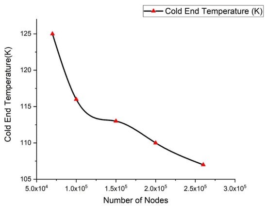
Figure 2.
Grid independence test of DIPTR.
For model validation, the findings of the existing numerical model was contrasted with the Biswa model [32] for the better improvement of results, and the validation is shown in Section 4 and also from the grid independence parameter mentioned in Figure 2, and accordingly convergence value is shown in Figure 3.
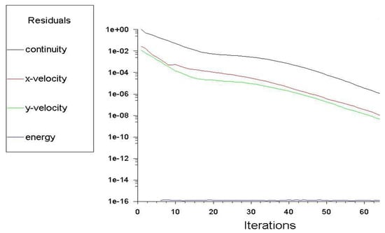
Figure 3.
Convergence criteria of DIPTR.
3. Results and Discussion
3.1. Effect of Phase Relation on Pressure and Mass Flow Rate for DIPTR
The DIPTR GM configuration was evaluated with specific load and limit conditions and varying opening values of the orifice valve and double-inlet valve for its best performance. Results of a CFD model over a constant duration of case 1, 2 and 3 are shown in Figure 4, for the interaction between the process of mass flow oscillation and oscillation pressure. The equation indicates that the oscillating mass flow rate, as well as the oscillating power, are systematic. In addition, it was clear from the figure that both oscillating pressure and oscillating mass flow were in phase. The difference in phase between the pressure and the mass flow rate for these three cases was 57°, 70° and 67°, respectively. As in case 1, it can be easily visualized that the phase difference was less as compared to the other cases 2 and 3, which have great phase difference and cannot give the minimum temperature at the cold end of the system which needs to be achieved. Thus, case 1 was considered good due to its less phase difference and thus minimum cold-end temperature can be achieved.
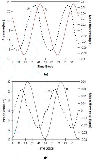
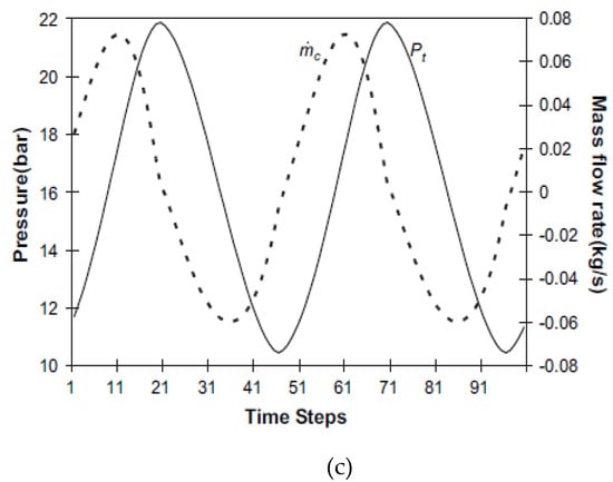
Figure 4.
Phase relation effect between pressure and mass flow rate: (a) Case 1; (b) case 2; (c) case 3.
3.2. Effect of DI Valve Opening for Different Cases
There were five simulation cases: Cases 1, 2 and 3 related to adiabatic boundary conditions with the different opening values of DIPTR; case 4 related to valve openings, and case 5 related to isothermal and specified boundary conditions for optimal valve opening. In order to study cooling efficiency, the effects of continuous simulacrum CFDs with adiabatic boundary conditions were studied. The first case is case 1, which corresponds to a 20% opening of the double-inlet valve and 30% opening of the orifice valve. Case 1 uses an adiabatic wall minimal state at the cold end, which does not equate to a complete cooling load on the device. Cases 2 and 3 were also valid for the other valve opening values, as shown in Table 2, and for the adiabatic surface boundary conditions.
Table 2.
Percentage of valve opening.
3.3. Effect of Cold-end Temperature and Time Step for Different Cases
At the cool end of the cycle, the average temperature changes over time are shown in Figure 5 for cases 1, 2 and 3. With the simulation time step, the cold-end temperature decreases gradually. The cyclic change of cold-end temperature after a certain time was constant. In other words, cold temperature with a simulation time does not drop anymore. This constant temperature is the minimum temperature of the device. After a 1600 s time steps simulation, the final cold-end temperature was 150 K for case 1. In cases 2 and 3, the minimum temperature at cold ends is 155 K and 200 K because it involved different percentages of valve opening (i.e., double-inlet valve and orifice valve). Case 1 shows the good and constant decrement of temperature at the time step of 1500 s, but for cases 2 and 3 it shows the irregularities of increasing and decreasing at different time steps. In addition, both cases did not reach the minimum temperature that was achieved for case 1.
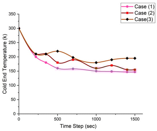
Figure 5.
Between cold load temperature and cases 1, 2 and 3.
3.4. Effect of Mass Flow Rate and Time Step for Different Cases
The cooling period in the individual systems was higher than expected arising from the inability to add the thermal mass in the systems. The cyclical steady state output of the simulation took around a month. In terms of thermodynamics, at an optimum opening of the double-inlet valve and the orifice valve at a specified frequency, the average enthalpy flow through the cycle should be maximum. Two reasons exist: First, the phase lag between the pressure and the mass flow rate was small; second, the mass flow rates in the pulse pipe section were larger, as shown in Figure 6. Case 1 was considered good because flow of mass was less, but flow was smooth as compared to cases 2 and 3 at the given boundary condition and valve opening percentages. In cases 3 and 2, mass flow rate was negative and showed irregularities of mass flow at different time steps, for example, at the time step of almost 65 s, cases 2 and 3 had a flow rate of -0.08 and case 1 had a flow rate of 0.01.
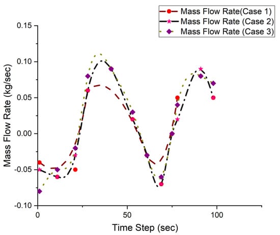
Figure 6.
Effect of mass flow rates through pulse tube cross section for cases 1–3.
3.5. Effect of Distribution of Average Temperaturealong Length of Pulse Tube
Figure 7 shows the average cycle temperature distribution throughout the pulse tube length. Case 1 had a good enthalpy from the cold end to the hot end that provides the device with a minimum temperature of the cold end. The figure shows the minimum temperature was reached at the cold end of the pulse pipe. As the length of pulse tube increases, the cold-end temperature (static temperature) decreases up to some extent, which provides the lowest temperature to achieve.
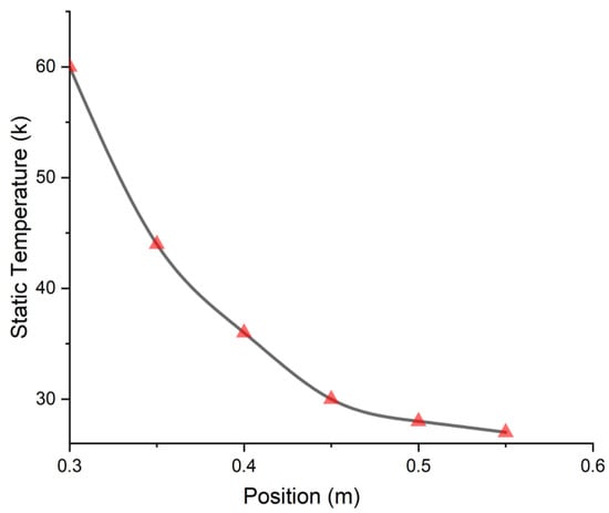
Figure 7.
Distribution of temperature along the length of pulse tube for case 1.
The contours of temperature and density along the simulated system length are shown in Figure 8.
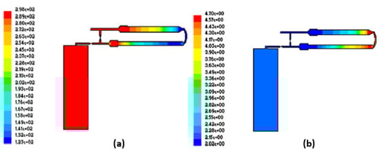
Figure 8.
(a) Temperature contour; (b) density contour.
The varying shades display the temperature and thickness of different parts of this contour diagram. The patterns are close to those documented in the literature of CFD simulations from specific PTR models. The temperature of the whole device was 293 K in this simulation initially, and the cold end of case 1 was kept at 2 Hz frequency at 150 K after a balanced periodical state was achieved. FLUENT tests the cold end in the above example to see whether cool-end temperature repeats from stage to stage. Figure 9 shows the velocity vectors in various sections of the pulse tube system to check that the process is continuous.
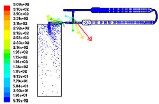
Figure 9.
Velocity vector for the entire system.
3.6. Heat Transfer Rate of CHX for Different Cases
This section addresses some of the significant observations of cases 4 and 5. Case 4 is the simulation of case 1 pulse tubing systems, with continuous heat load from adiabatic wall pressure to the 1 W heat exchanger of the cold end; the same as the 1 W refrigeration load system. The simulation started at an estimated 293 K temperature and continued until it was constantly maintained. Figure 10 shows the average system level of heat output. The positive value of the mean heat output of the process is shown. At time steps of 5 to 15 s, the heat transfer rate was up to -1000 because working fluid was injected through the inlet. Then the process starts at the time step of 20 s, whereby the heat transfer rate was 0, as the system was in moderate state; after that the rate of heat transfer increases up to 2000 at the time step of 35s. This cycle of heat transfer is shown in Figure 10, where the decrement at the time step of 40s can be observed.
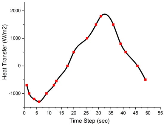
Figure 10.
Rate of heat transfer over a cycle at CHX for case #5.
The cooling temperature was expected to reach 130 K. For case number 1, the cold heat exchanger maintains a steady surface temperature of 150 K. In this scenario, the heat load of reaching the cold end was measured due to the enforced cold-end isothermal wall boundary state. Therefore, the energy distributions of the cold-end wall should be called stable-periodical, as they are repeated from cycle to cycle. A cooling load of 3.7W was achieved in a stable, periodic phase, based on the simulation’s performance. That was, the system has 3.733 W of cooling capacity at a functioning cold temperature of 150 K.
4. Validation of Results
This section describes some important comparisons of parameters with experimental data such as cooling behavior, cooling energy, axial temperature variation and regenerator inlet pressure waves [33]. However, in Section 4.1, Section 4.2 and Section 4.3 the discrepancy between the numerical and experimental values was due to the unaccounted inefficiency losses in the system, due to the two-dimensional simulation model taken for the simulation and neglecting the wall thickness of the system in the simulation. The model was considered validated with error because the experimental data also has some error during experimentation due to the changing of surrounding conditions (i.e., temperature of the lab where these experiments were conducted), but in simulation these conditions were not considered. That is why this model was considered validated and some researchers also had these validation errors, as reported in the literature [34].
4.1. Cooling Behavior
The CFD research comparisons with the DIPTR system’s experimental results for cooling down behavior of the system is shown in Figure 11. With the increment of time step, the cooling temperature decreases, but the test results and CFD simulation results differ significantly, as the simulation results at the time step of 1.0 s cold-end temperature was almost 149K but for experimental data it was 200 K, which was a bit high from the simulation results.
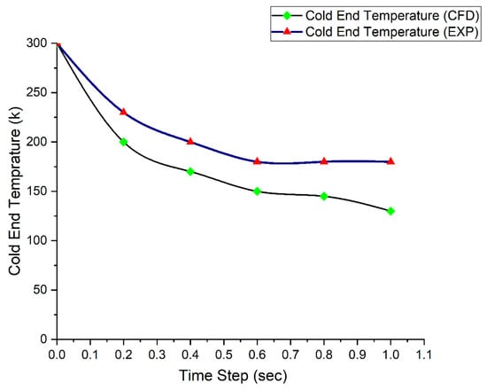
Figure 11.
Comparison of cold-end temperature of DIPTR with time step for case 1.
4.2. Cooling Energy
The figure shows a strong reflection on the effects of the CFD and the outcomes of studies. Figure 12 indicates the connection between the experimental results and the output of the CFD model of the cooling energy or heat load. For the simulation results at the time step of 08 s, the cooling energy increases as more heat was dissipated when the cold-end temperatures decreases to 150 K, but experimental results were a bit high because of less dissipation of heat and the temperature was 200K.
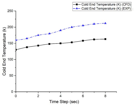
Figure 12.
Comparison of heat load and cooling energy of DIPTR for case 1.
The theoretical and experimental values demonstrate the contrast between the cooling activity and the cooling energy arising from non-reporting efficiency losses in this process, as well as a two-dimensional template simulation prototype used to simulate and ignore the walls of the structure.
4.3. Pulse Tube Length
Temperature distribution differences between experimental and CFD simulation over the length of the pulse tube are shown in Figure 13. This shows a good difference of gradual increments of length when temperature decreases, and after some time reached its minimum. As the length increases the temperature at the cold end was decreased; at 0.25 m of length of pulse tube, the temperature drops to 140K for CFD results and for experimental results it was 220K, which was a bit high from the simulation results.
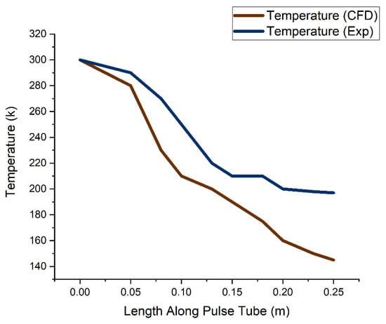
Figure 13.
Comparison of variation of temperature along the pulse tube length.
4.4. Regenerator Pressure Inlet
Similarities in the GM-type DIPTR regenerator inlet for the prototype and CFD simulator pressure wave forms shown in Figure 14. The experimental wave was found between the sinusoidal and rectangular forms, although the pressure wave structure was sinusoidal for simulation results at time steps of 50, 100 and 150 s. All waves had the same amplitude.
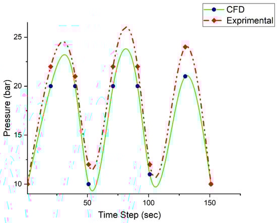
Figure 14.
Comparison of pressure at the regenerator inlet of DIPTR.
5. Conclusions
In the UDF, a DIPTR with different valve openings and boundary conditions, as previously described, had different cooling performances. Three different simulation results were tested for the entire DIPTR process. The specified temperature was considered thermal load by the cold-end heat exchanger. Three cases were studied to model the valve openings for adiabatic cold-end environments. Simulation ends at the expected temperature of the system and was still under intermittent constant conditions. The CFD model effectively predicts the pulse-tube cooler component comfortability by resolving the Navier–Stokes equations for fluid dynamics and heat transfer and an excellent gas composition for the state system. Unlike other valve-open standards, with a 20% DI valve opening and 30% opening of orifice valve, the DIPTR model offers greater versatility for better efficiency and performance. In case of re-powered temperatures of 150 K, the load will be 3.7W. The changes in the mass flow rate of the pulse tube and the phase relation in the pulse tube can be explained. In this current research, it was also demonstrated that the energy component for cooling energy was successfully confirmed between prior experimental results and CFD simulations. Comparisons of other variables prove that the CFD model was acceptable and the test results were a bit improved from experimental results. This simulation proves very beneficial in the industrial application of gas liquefaction, surveillance and in the medical area, such as in MRI machines for the cooling of the system, which are in a running state without any breaks. This causes the decrement of efficiency of the system due to high usage. Moreover, these results can more precisely be improved in future by putting different boundary conditions on a 3-D simulation model. Furthermore, changing the working medium proved beneficial for achieving low temperature at the cold end.
Author Contributions
Conceptualization, M.A. and M.F.; methodology, U.S. and M.F.; software, M.A. and Z.-u.-R.T.; validation, S.N. and N.W.; formal analysis, M.F. and S.R.N.; investigation, M.F. and Q.A.; resources, M.N. and M.S.T.; data curation, I.A.C. and J.M.A.; writing—original draft preparation, M.A. and M.F.; writing—review and editing, M.F., A.A., M.N. and S.R.N.; supervision, M.F.; project administration, M.F., S.R.N. and M.N. All authors have read and agreed to the published version of the manuscript.
Funding
This research work did not receive any external funding.
Conflicts of Interest
The authors declares no conflicts of interest.
References
- Kumar, P.; Gupta, A.K.; Kumar, M.; Sahoo, R.K. Numerical investigation to predict the performance of a GM pulse tube refrigerator using of pressure wave profile GM pulse tube refrigerator. Mater. Sci. 2018, 6, 1–7. [Google Scholar]
- Gujarati, P.B.; Desai, K.P.; Naik, H.B.; Atrey, M.D. Transient analysis of single stage GM type double inlet pulse tube cryocooler. In IOP Conference Series: Materials Science and Engineering; no. 1; IOP Publishing: Bristol, UK, 2015; Volume 101, p. 012033. [Google Scholar]
- Kumar, P.; Gupta, A.K.; Sahoo, R.K.; Jena, D.P. Numerical investigation of a 3D inertance pulse tube refrigerator from design prospective. Cryogenics 2019, 98, 125–138. [Google Scholar] [CrossRef]
- Wang, W.; Hu, J.; Xu, J.; Zhang, L.; Luo, E. Influence of the water-cooled heat exchanger on the performance of a pulse tube refrigerator. Appl. Sci. 2017, 7, 229. [Google Scholar] [CrossRef]
- Liu, X.; Chen, C.; Huang, Q.; Wang, S.; Hou, Y.; Chen, L. Modeling of heat transfer and oscillating flow in the regenerator of a pulse tube cryocooler operating at 50 Hz. Appl. Sci. 2017, 7, 553. [Google Scholar] [CrossRef]
- Hamood, A.; Jaworski, A.J.; Mao, X. Development and assessment of two-stage thermoacoustic electricity generator. Energies 2019, 12, 1790. [Google Scholar] [CrossRef]
- Roy, P.C.; Kundu, B. Thermodynamic modeling of a pulse tube refrigeration system. J. Therm. Eng. 2018, 4, 1668–1679. [Google Scholar] [CrossRef]
- Tang, K.; Feng, Y.; Jin, T.; Jin, S.; Yang, R. Impact of Gedeon streaming on the efficiency of a double-inlet pulse tube refrigerator. Appl. Therm. Eng. 2017, 111, 445–454. [Google Scholar] [CrossRef]
- Antao, D.S.; Farouk, B. Computational fluid dynamics simulations of an orifice type pulse tube refrigerator: Effects of operating frequency. Cryogenics 2011, 51, 192–201. [Google Scholar] [CrossRef]
- Liu, D.; Dietrich, M.; Thummes, G.; Gan, Z. Numerical simulation of a GM-type pulse tube cryocooler system: Part II. Rotary valve and cold head. Cryogenics 2017, 81, 100–106. [Google Scholar] [CrossRef]
- Kim, K.; Zhi, X.; Qiu, L.; Nie, H.; Wang, J. Analyse numérique des différents effets des vannes sur les performances de refroidissement d’un refroidisseur cryogénique à tube à pulsation de type Gifford-McMahon à deux étages. Int. J. Refrig. 2017, 77, 1–10. [Google Scholar] [CrossRef]
- Ashwin, T.R.; Narasimham, G.S.V.L.; Jacob, S. CFD analysis of high frequency miniature pulse tube refrigerators for space applications with thermal non-equilibrium model. Appl. Therm. Eng. 2010, 30, 152–166. [Google Scholar] [CrossRef]
- Zhu, S.W.; Chen, Z.Q. Isothermal model of pulse tube refrigerator. Cryogenics 1994, 34, 591–595. [Google Scholar] [CrossRef]
- Moldenhauer, S.; Thess, A.; Holtmann, C.; Fernández-Aballí, C. Thermodynamic analysis of a pulse tube engine. Energy Convers. Manag. 2013, 65, 810–818. [Google Scholar] [CrossRef]
- Yang, S.; Wu, Y.N.; Zhou, Z.P.; Jiang, Z.H.; Zhang, A.K. Simulation and Experimental Analysis of Pulse Tube Refrigerator with an Active Phase Controller; International Cryocooler Conference, Inc.: Boulder, CO, USA, 2016; pp. 211–218. [Google Scholar]
- Dang, H.; Zhao, Y. CFD modeling and experimental verification of a single-stage coaxial Stirling-type pulse tube cryocooler without either double-inlet or multi-bypass operating at 30–35 K using mixed stainless steel mesh regenerator matrices. Cryogenics 2016, 78, 40–50. [Google Scholar] [CrossRef]
- Yu, H.; Wu, Y.; Ding, L.; Jiang, Z.; Liu, S. An efficient miniature 120 Hz pulse tube cryocooler using high porosity regenerator material. Cryogenics 2017, 88, 22–28. [Google Scholar] [CrossRef]
- Arunkumar, K.N.; Kasthuriregan, S.; Vasudevan, K. Numerical analysis of single stage pulse tube refrigerator. Int. J. Eng. Technol. 2017, 9, 3798–3805. [Google Scholar]
- Abraham, D.; Damu, C.; Kuzhiveli, B.T. Numerical analysis of inertance pulse tube cryocooler with a modified reservoir. IOP Conf. Ser. Mater. Sci. Eng. 2017, 278, 012154-62, No. 1. [Google Scholar] [CrossRef]
- Gour, A.S.; Sagar, P.; Karunanithi, R. Design, development and testing twin pulse tube cryocooler. Cryogenics 2017, 86, 87–96. [Google Scholar] [CrossRef]
- Cao, Y.; Chen, X.; Wu, Y. Theoretical and experimental investigation of two pulse tube cryocoolers driven by a single opposed linear compressor. Cryogenics 2014, 61, 154–157. [Google Scholar] [CrossRef]
- Gifford, W.E.; Longsworth, R.C. Pulse-Tube Refrigeration. ASME. J. Eng. Ind. 1964, 86, 264–268. [Google Scholar] [CrossRef]
- Krishnappa, G.B.; Madhu, D.; Kasthurirengan, S. Comparison of 1D and 2D flow numerical analysis applied to two stage pulse tube cryocooler. In AIP Conference Proceedings; No. 1; American Institute of Physics: College Park, MD, USA, 2012; Volume 1434, pp. 1157–1164. [Google Scholar]
- Liu, S.; Chen, X.; Zhang, A.; Kan, A.; Zhang, H.; Wu, Y. Impact of coiled type inertance tube on performance of pulse tube refrigerator. Appl. Therm. Eng. 2016, 107, 63–69. [Google Scholar] [CrossRef]
- Antao, D.S.; Farouk, B. Experimental and numerical investigations of an orifice type cryogenic pulse tube refrigerator. Appl. Therm. Eng. 2013, 50, 112–123. [Google Scholar] [CrossRef]
- Rout, S.K.; Behura, A.K.; Dalai, S.; Sahoo, R.K. Numerical analysis of a modified type pulse tube refrigerator. Energy Procedia 2017, 109, 456–462. [Google Scholar] [CrossRef]
- Sosso, A.; Durandetto, P. Experimental analysis of the thermal behavior of a GM cryocooler based on linear system theory. Int. J. Refrig. 2018, 92, 125–132. [Google Scholar] [CrossRef]
- Cai, J.H.; Zhou, Y.; Wang, J.J.; Zhu, W.X. Experimental analysis of double-inlet principle in pulse tube refrigerators. Cryogenics 1993, 33, 522–525. [Google Scholar] [CrossRef]
- Dai, Q.; Chen, Y.; Yang, L. CFD investigation on characteristics of oscillating flow and heat transfer in 3D pulse tube. Int. J. Heat Mass Transf. 2015, 84, 401–408. [Google Scholar] [CrossRef]
- Rout, S.K.; Gupta, A.K.; Choudhury, B.K.; Sahoo, R.K.; Sarangi, S.K. Influence of porosity on the performance of a pulse tube refrigerator: A CFD study. Procedia Eng. 2013, 51, 609–616. [Google Scholar] [CrossRef]
- Banjare, Y.P.; Sahoo, R.K.; Sarangi, S.K. CFD simulation of a Gifford-McMahon type pulse tube refrigerator. Int. J. Therm. Sci. 2009, 48, 2280–2287. [Google Scholar] [CrossRef]
- Biswas, A.; Ghosh, S.K. Experimental and numerical investigation on performance of a double-inlet type cryogenic pulse tube refrigerator. Heat Mass Transf. Stoffuebertragung 2016, 52, 1899–1908. [Google Scholar] [CrossRef]
- Das, P.C.; Roy, S.K.; Sarangi, P.K. Some Theoretical and Experimental Studies on Pulse Tube Refrigeration; IIT: Kharagpur, India, 2004. [Google Scholar]
- Banjare, Y.P.; Sahoo, R.K.; Sarangi, S.K. CFD simulation and experimental validation of a GM-type double-inlet pulse tube refrigerator. Cryogenics 2010, 50, 271–280. [Google Scholar] [CrossRef]


© 2020 by the authors. Licensee MDPI, Basel, Switzerland. This article is an open access article distributed under the terms and conditions of the Creative Commons Attribution (CC BY) license (http://creativecommons.org/licenses/by/4.0/).