Fault Detection and Isolation for a Cooling System of Fuel Cell via Model-based Analysis

Abstract

The development of fuel cell electric vehicles in recent years has led to increased interest in the use of fuel cells as sources of renewable energy. To achieve successful commercialization of fuel cell vehicles, it will be necessary to guarantee the safety, reliability, and lifetime of fuel cell systems by predictive fault detection and isolation (FDI). In this study, the parity equation, an observer, and a Kalman filter are employed together to compare the characteristics of FDI, focusing on the sensors of the thermal management system. Residuals corresponding to the difference between temperature outputs of linear models under driving cycles and nonlinear temperature outputs are used to isolate faults. Then, assessment of three model-based sensor FDI schemes is used to isolate sensor faults using the Cumulative Sum Control Chart (CUSUM) method. Generated residuals are evaluated by CUSUM to detect the presence of a sensor fault. As a result, isolated sensor faults are assessed.

1. Introduction

The development of fuel cell electric vehicles (FCEVs) in recent years has led to increased interest in the use of fuel cells as sources of renewable energy for fuel cell vehicles, owing to their high efficiency, low pollution, and good power density [1,2,3,4,5,6]. Proton exchange membrane fuel cell (PEMFC) systems are widely applied to fuel cell vehicles because of their quick fuelling and extended running time [7,8].

To achieve commercialization, however, it will be necessary to solve technical issues related to the safety, reliability, and lifetime of fuel cell systems [9,10]. For commercialization, automakers around the world are targeting 5000 h of operation for transportation applications by 2020. However, according to a research survey, 78% of fuel cell vehicles did not exceed 2000 h of durability. Especially, since the reliability and durability affect human safety during vehicle operation, many researchers have performed durability tests and faults diagnosis. In addition, fault detection and fault diagnosis have become more important at the system level, in particular because fuel cell systems such as air supply, fuel supply, thermal management, power converter, etc., are dependently operated, and thus a fault in any subsystem can damage the entire fuel cell vehicle system. Therefore, it is necessary to detect initial faults early, before a minor fault becomes a serious fault.

A few researchers have attempted to address the FDI of fuel cell systems using model-based methods. Pei et al. investigated water fault diagnosis-based pressure drop using different indicators. They reviewed recent studies on the use of pressure drop, as found in calculation results, to diagnose water fault [11]. Shao et al. presented an ANN (artificial neural network) ensemble method to diagnose faults of PEMFC. They verified the efficiency of the fault diagnosis method [12]. Pahon et al. proposed a novel signal-based approach for PEMFC fault diagnosis. The proposed method performed verification with experimental data for faults of the air management system [13]. A model-based fault diagnosis method was designed by Escobet et al. based on computing residuals and binary signature matrixes of analytical residuals [14]. Li et al. proposed a novel data-driven fault diagnosis method and diagnosis rule for PEMFC [15,16]. Puig et al. reported the MPC (Model Predict Control) algorithm to control the oxygen excess ratio under compressor voltage and air valve opening area faults [17]. Philippe et al. reported a DoE (Design of Experiments) diagnostic for faulty water management, and they also determined the ageing parameters of the fuel cell [18]. A fault detection and isolation algorithm using a model-based diagnostic algorithm was presented by Polverino et al. Simulations in a software environment were performed on sensor and actuator faults. [19]. Rosich et al. proposed model-based fault detection and isolation (FDI) for PEM fuel cell systems [20]. Zhang et al. presented fault detection methodology using the state space model of hybrid DC power sources [21]. Through a case study, Lira et al. illustrated model-based fault detection using an LPV(Linear Parameter-Varying) design that was linearized for non-linear fuel cell systems using Jacobian linearization and fault scenarios [22]. Kamal et al. designed an RBF (radial basis function) to improve the sensitivity of residuals for one actuator fault and three sensor faults [23]. Even though PEMFC fault detection and isolation methods have been reported in the literature, previous studies have generally considered only certain limited approaches to analysing the fuel cell vehicle system.

In fuel cell vehicle systems, various faults can occur not only in the sensors but also in the actuators. Especially, the temperature of the stack and coolant is closely related to stack durability and performance. Particularly for a fuel cell vehicle system, the system temperature must be properly regulated due to frequent heat release caused by load variations. Thus, it is important to detect sensor faults of the thermal management system before the stack degrades and stack performance drops.

Fault detection algorithms are generally categorized as either model-based or hardware-based approaches. Since hardware redundancy and the associated cost are disadvantageous, model-based approaches are preferred. The model-based approaches include the parity equation method, state observer method, and Kalman filter method. Model-based approaches reduce the number of hardware components such as sensors, as well as the system costs.

The parity relation method involves easy design of parity equations to generate a residual without state estimation. However, the model should work with linear fuel cell systems. The state observer method can overcome the drawbacks of the parity relation but may lead to system noise and disturbances. A Kalman filter is useful to detect sensor faults via noise-free measurements; it is also robust and simple. However, it is challenging to implement Kalman filters for nonlinear systems.

In this study, the parity equation, observer, and Kalman filter methods were employed together to compare the characteristics of the FDI residual. Then, an assessment of three model-based sensor FDI schemes is used to isolate a sensor fault using the Cumulative Sum Control Chart (CUSUM) method. Two sensor fault scenarios are selected—one for stack temperature sensor faults, the other for coolant inlet temperature sensor faults. The three methods are applied to detect a temperature sensor fault and, to generate a residual, the output signal in the normal operating model is compared with the output signal in the model-based FDI schemes. The generated residual is evaluated using CUSUM to detect the presence of a sensor fault. Finally, the isolated sensor fault is assessed.

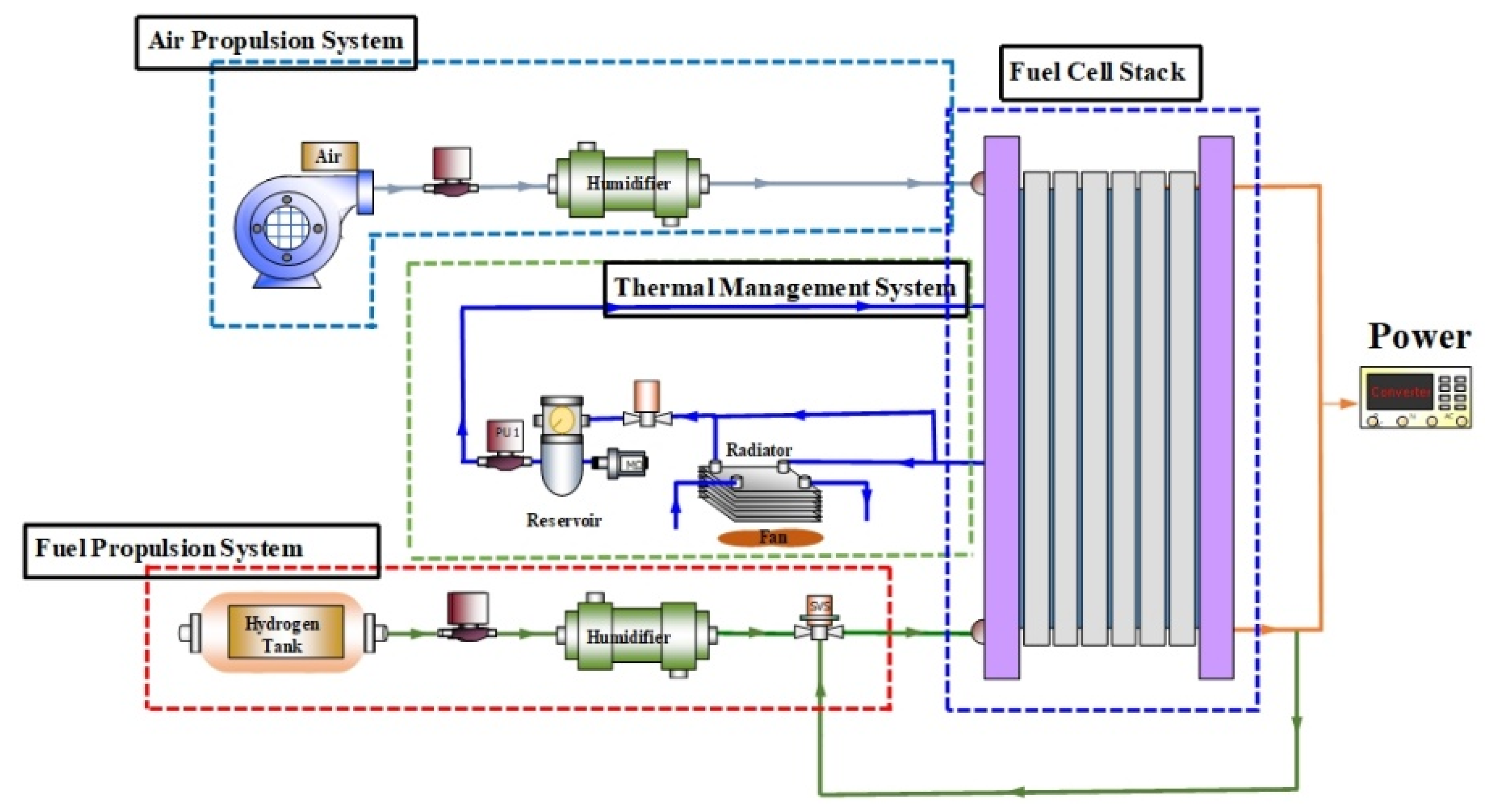
2. Nonlinear Model for Normal Operation Conditions

The model-based fault detection and isolation algorithm requires a nonlinear fuel cell model to capture the electrochemical properties and perform fault detection and isolation. The lumped parameter approach is incorporated into the stack model to mitigate the otherwise high computational load. As a compromise for the accuracy of the designed model and to reduce the computational load, the model is validated with testing data. The fuel cell system model is composed of a dynamic blower with a motor, a dynamic fuel cell stack, a humidifier, a hydrogen tank, and a cooling system, as shown in Figure 1. More detailed nonlinear fuel cell models can be found in previous studies [24,25,26].

The design of the nonlinear dynamic fuel cell models assumes:

• The fuel on the anode side contains hydrogen and water vapour and the air on the cathode side contains oxygen, nitrogen, and water vapour;
• In the humidifier model, the injected water is vaporized without heat losses;
• Both the fuel and air were assumed to be ideal gases;
• The temperature in the fuel cell stack is uniform; and
• The electrochemical reaction is quasi-steady.

2.1. Fault Free Model of Fuel Cell System

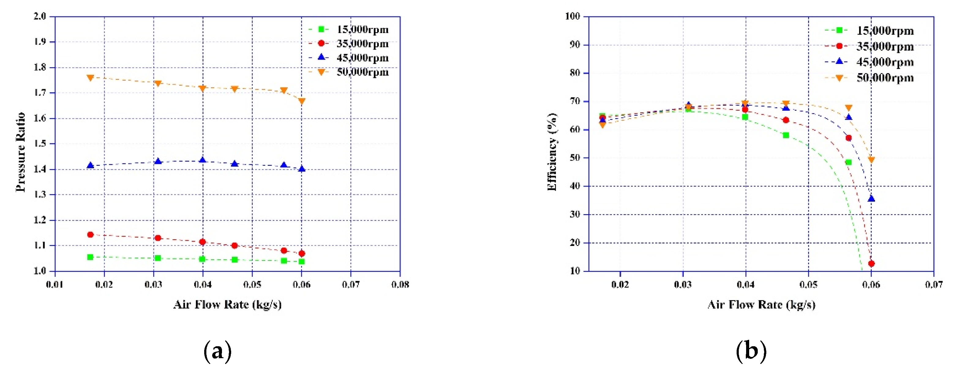
2.1.1. Air Supply Model

Air is supplied to the stack with a blower. A semiempirical model is applied to build a model of a turbo blower. The experimental data were obtained from Franklin et al. [27], and the performance curve and efficiency of the blower are shown in Figure 2a,b. The experimental data for the blower were provided in the form of a look-up table. The blower is operated by a DC motor. The model of the dynamic electric motor was derived from the specification data [24]. In addition, the PI controller regulates the motor speed to maintain an oxygen excess ratio of 2.2.

2.1.2. Hydrogen Supply Model

The anode fuel flow includes the hydrogen flow rate and the humid vapour. The inlet anode mass flow rate into the stack is calculated as

$${\dot{m}}_{H_2,in}=\frac{J}{2F}\times A\times n\times st{o}_{H_2}\times M_{H_2}$$

(1)

where J is the current density, sto_H2 is the hydrogen stoichiometry ratio, A is the active area through the cell, and n is the number of cells. The relative humidity ϕ_in,an at the anode inlet is calculated as

$${\varphi }_{in,an}=\frac{y_{H_{2}O,in,an}\times p_{in,an}}{p_{sat}\times M_{H_{2}O}}$$

(2)

where y_H2O,in,an is the mass fraction of vapor at the anode side, M_H2O is the molecular weight of water, and p_sat is the saturation pressure.

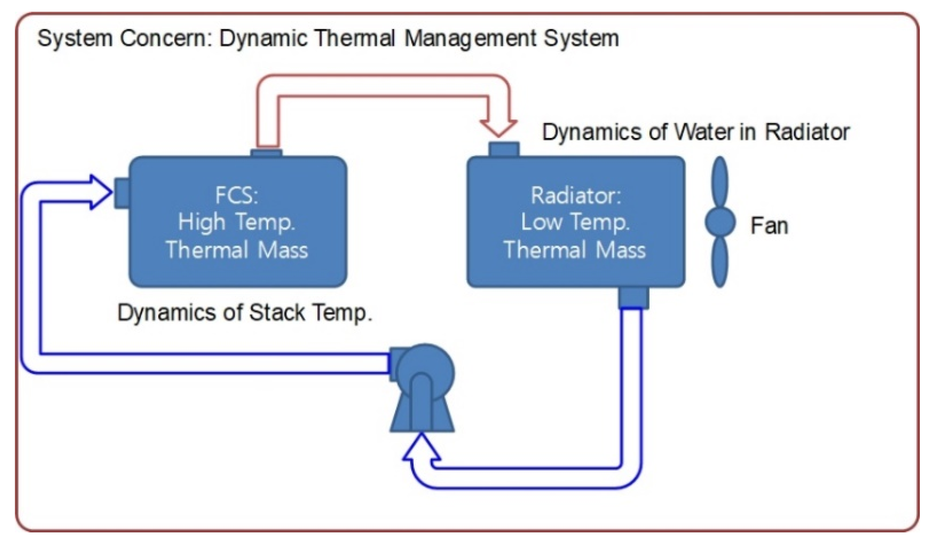
2.1.3. Dynamic Model

A dynamic model of the fuel cell stack is designed to implement the sensor fault scenario. The stack model assumes a lumped mass for the dynamic response of thermal energy input. The lumped stack obtains heat from the electrochemical reaction (${\dot{H}}_{rea}$) and the heat is rejected via convection heat transfer to the surroundings (${\dot{Q}}_{surr}$), involving gases exhausted from the anode channel and the cathode channel (${\dot{Q}}_{gas}$), and convection in the water coolant (${\dot{Q}}_{cool}$). The stack model is as follows [28]:

$$m_{sta}{c}_{p,sta}{\dot{T}}_{sta}={\dot{H}}_{rea}-{\dot{Q}}_{gas}-{\dot{Q}}_{cool}-{\dot{Q}}_{surr}$$

(3)

where m_sta, and c_p,_sta are the mass and the specific heat of fuel cell stack, and ${\dot{T}}_{sta}$ is the stack temperature.

A dynamic cooling reservoir model is also developed. The water in the fuel cell stack and cooling circuit is considered as a lumped mass. The reservoir is assumed to be placed at the inlet of the fuel cell stack. The governing equation of the coolant reservoir, then, is

$$m_{c,Rv}{c}_{p,Rv}{\dot{T}}_{RV}=c_{p,c}{\dot{m}}_c\left(T_{mix}-T_{RV}\right)$$

(4)

where m_c,Rv, c_p,_RV is the mass of reservoir, and specific heat of reservoir, T_RV is the reservoir temperature. T_mix is the sum of coolant outlet temperature through the stack and the radiator.

The total mass of water present in the reservoir, radiator, and cooling channel of the stack is 7 kg. A bypass valve and radiator fan are used to control the coolant inlet temperature. The dynamic thermal management system with fault diagnosis is shown in Figure 3.

2.1.4. Electrochemical Reaction Model

The fuel cell stack produces electric power and heat by chemical reaction. When the fuel cell stack is requested to supply power, electric power is determined by the current and the electric potential. The electric potential of the fuel cell stack is calculated by the following equation:

$$V_{sta}=\left(V_{nern}-J\cdot R{(\lambda )}_{mem}-V_{act}\right)\times n_{cell}$$

(5)

where V_sta is stack voltage, R is electric resistance, λ is water content, and V_act is activation loss; the Nernst voltage, V_nern, is described as follows [25]:

$$V_{nern}=1.229-8.5\times {10}^{-4}\cdot \left(T_{sta}-298.15\right)+4.308\times {10}^{-5}\times T_{sta}\times \left(\ln p_{H_2}+0.5\ln p_{O_2}\right)$$

(6)

In Equation (5), the activation loss V_act can be expressed as follows [26,29].

$$V_{act}={\epsilon }_1+{\epsilon }_2{T}_{sta}+{\epsilon }_3{T}_{sta}\left[\ln \left(c_{O_2}\right)\right]+{\epsilon }_4{T}_{sta}\left[\ln \left(I/n\right)\right]$$

(7)

where ε is a tuning factor that can be adjusted by experimental data (ε₁ = −0.5708, ε₂ = 0.0017, ε₃ = 0.000017903, ε₄ = −0.0001) and $c_{O_2}$ is the oxygen concentration at the cathode.

The Ohmic loss is expressed by the ionic resistance in the membrane. This loss term is applied in Equation (5) in terms of the water content (λ). The electric resistance in the membrane can be expressed as follows [29]:

$$R{(\lambda )}_{mem}={\displaystyle {\int }_{z=0}^{z=t_{mem}}\frac{1}{\exp \left[1268\left(\frac{1}{303}-\frac{1}{T_{sta}}\right)\right]\left(0.005139\lambda -0.000326\right)}dz}$$

(8)

where z is membrane thickness.

2.2. State Variables for Design of FDI

For sensor FDI, the state variables in our study are the temperature of the fuel cell stack and the coolant inlet temperature. The selected state variables can be represented in nonlinear state space form.

$$\tilde{\dot{x}}=[\begin{array}{cc}{\tilde{\dot{T}}}_{sta}& {\tilde{\dot{T}}}_{RV}\end{array}]=\left[\begin{array}{cc}{\tilde{\dot{x}}}_1& {\tilde{\dot{x}}}_2\end{array}\right]$$

(9)

The coolant flow rate and the opening area of the bypass valve are employed as the manipulated variables:

$$\tilde{u}=[\begin{array}{cc}{\tilde{m}}_c& k\end{array}]=\left[\begin{array}{cc}{\tilde{u}}_1& {\tilde{u}}_2\end{array}\right]$$

(10)

The output variables are the same as the state variables:

$$\tilde{y}=[\begin{array}{cc}{\tilde{\dot{T}}}_{sta}& {\tilde{\dot{T}}}_{RV}\end{array}]=\left[\begin{array}{cc}{\tilde{y}}_1& {\tilde{y}}_2\end{array}\right]$$

(11)

Disturbances are the result of fluctuation of current and ambient temperature:

$$\tilde{d}=[\begin{array}{cc}\tilde{I}& {\tilde{T}}_{amb}\end{array}]=\left[\begin{array}{cc}{\tilde{d}}_1& {\tilde{d}}_2\end{array}\right]$$

(12)

Thus, the state and measurement equations in the nonlinear system are rewritten using Equation (9):

$$\{\begin{array}{l}\tilde{\dot{x}}(t)=f(\tilde{x}(t),\tilde{u}(t))+w(t)\\ \tilde{y}(t)=g(\tilde{x}(t),\tilde{u}(t))+v(t)\end{array}$$

(13)

where f($\tilde{x}$(t), $\tilde{u}$(t)) is the nonlinear system function and g($\tilde{x}$(t), $\tilde{u}$(t)) is the nonlinear measurement function; w(t) and v(t) are the Gaussian white noise and the covariance of the measurement noise, respectively.

3. Application of Fault Detection and Isolation

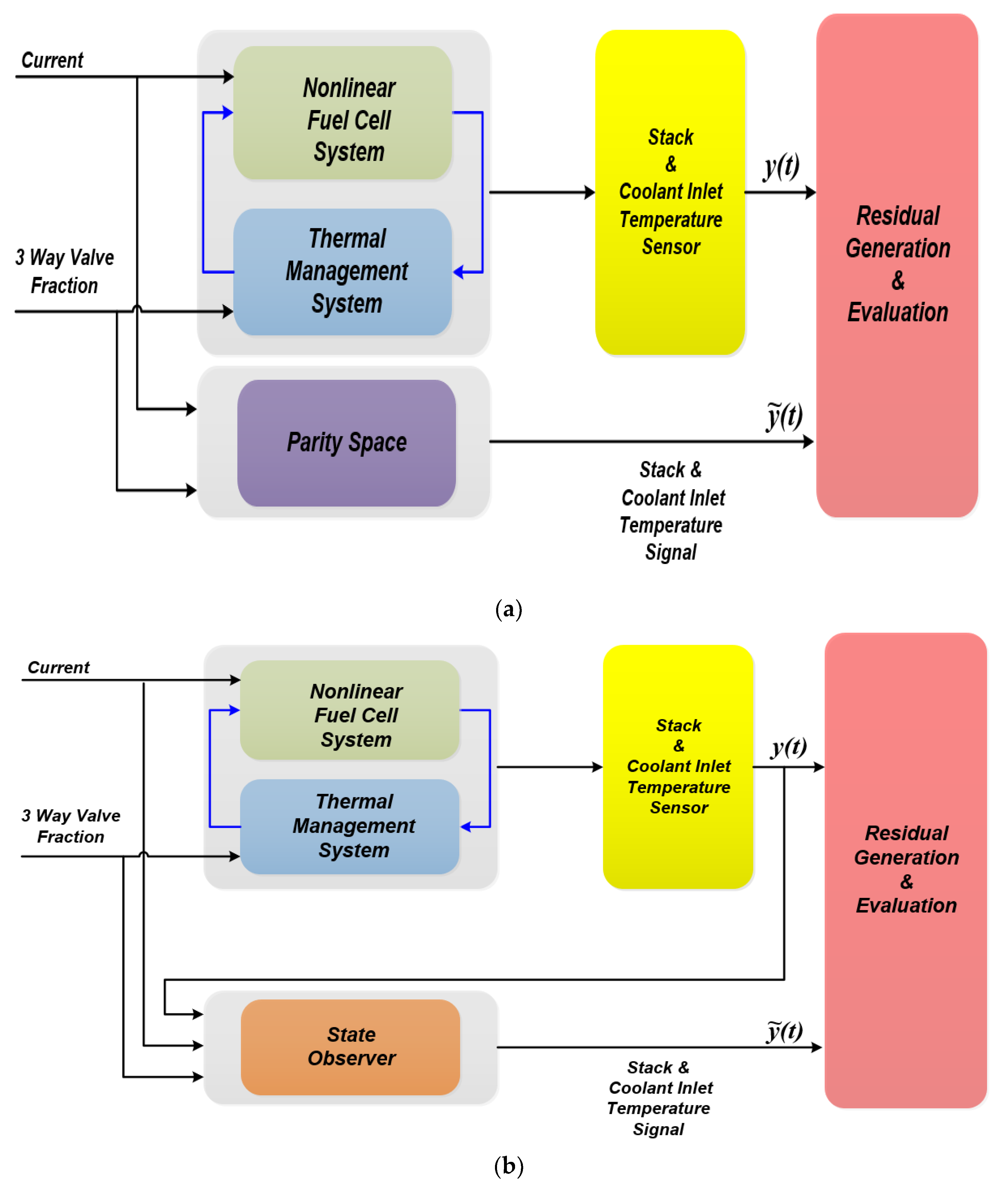
3.1. Scheme of Model-Based FDI

The fault detection and isolation algorithms of the temperature sensors applied in our study are a parity space, a state observer, and a Kalman filter, shown in Figure 4. Sensor faults in a fuel cell system are diagnosed by detection algorithms, in parallel with the nonlinear fuel cell system model, based on inputs such as the current and the bypass valve fraction. The residual is a clue allowing us to judge sensor faults; residuals are generated by comparing the outputs of the nonlinear fuel cell system to the outputs of the parity space, state observer, and Kalman filter. When a fault is detected, the residual signal shows trends different from the regular pattern. Since the trends vary according to the algorithms, it is necessary to evaluate sensor faults by established criteria. In Figure 4, while the parity space algorithm produces residuals independently from the inputs, the state observer and Karman Filter deliver their output to the healthy model. Those outputs are used to evaluate signal faults.

3.2. Fault Definition Model

The stack temperature and coolant inlet temperature are key control factors for the thermal management system (TMS) of a fuel cell. Thus, this study considers sensor faults regarding the stack temperature and coolant inlet temperature. In Equation (14), f_s is the sensor fault in the stack temperature sensor, and the coolant inlet sensor of the fuel cell.

In this study, two typical sensor faults are presented. Fault types are stuck and scaling, due to sensor core degradation and external shock or vibrations [30]. A stuck fault has a constant value caused by flaws resulting from sensor degradation during normal operation. Scaling is assumed to be in a form that does not change. Thus, the stuck and scaling faults can be considered additive faults, and can be expressed by the following equation:

$$y(t)=x+f_s+noise$$

(14)

where x is a state variable that represents the stack temperature or the coolant inlet temperature, y is the corresponding sensor measurement, and f_s is the sensor fault variable.

3.3. Model-Based FDI Design

3.3.1. Design of Parity Space Algorithm

The parity space approach is an open-loop method, one that utilizes analytical redundancy. It is based on the discrete state space model expressed by Equation (14). This equation is established to link the sensor outputs and inputs, as follows [31]:

$$Y(k)=Tx(k)+H_{u}U(k)+H_{w}W(k)+H_{v}V(k)+H_{f}F(k)$$

(15)

where T, H_u, H_w, H_v, and H_f are the related matrices, and, Y(k) is the temperature sensor output.

In this study, a first-order discrete linear dynamic model is used, consisting of two inputs, two disturbances, and two outputs. The state variables are directly output. The detailed matrices T, H_u, U, Y, and F are as follows:

$$T=\left(\begin{array}{l}C\\ CA\end{array}\right),H_u(k)=\left(\begin{array}{ccc}0& 0& 0\\ B& 0& 0\\ AB& B& 0\end{array}\right),U(k)=\left(\begin{array}{c}{u}_0\\ u_1\end{array}\right),Y(k)=\left(\begin{array}{c}{y}_0\\ y_1\end{array}\right),F(k)=\left(\begin{array}{c}{f}_0\\ f_1\end{array}\right)$$

(16)

3.3.2. Design of State Observer Algorithm

A linearized model was derived to implement the sensor FDI for thermal management of the fuel cell. The linear fuel cell system was developed in our previous study [31]. The nonlinear model was linearized by a Gaussian Jacobian method along the reference operating point. The vector $\dot{x}$(t), which depends on the states x₁ and x₂, is approximated by

$${\dot{x}}_i(t)=\approx {\dot{x}}_{ref}(t)+{\frac{d{h}_i}{d{x}_1}|}_{x=x_{ref}}(x_1-x_{1,ref})+{\frac{d{h}_i}{d{x}_2}|}_{x=x_{ref}}(x_2-x_{2,ref})$$

(17)

After the nonlinear state space form is redesigned into a continuous state space form, the state space representation of dynamic temperature that includes the sensor fault term is rewritten as follows:

$$\begin{array}{l}\dot{x}(t)=Ax(t)+B(u(kt+d(t))+w(t)\\ y(t)=C(t)+F{f}_s(t)+v(t)\end{array}$$

(18)

where F is assumed to be a known matrix, and f_s is the magnitude of the sensor faults. The system matrix form is defined as follows:

$$\mathrm{A}=\left[\begin{array}{cc}-0.1028& 0.0923\\ 0.7979& -1.0257\end{array}\right]\mathrm{B}=\left[\begin{array}{cc}-0.8001& 0\\ 5.3641& -3.7828\end{array}\right]\mathrm{C}=\left[\begin{array}{cc}1& 0\\ 0& 1\end{array}\right]$$

(19)

The state observer approach uses the output error between the estimated output and the model output. Hence, the linear fuel cell model was used to design the state observer. Among other approaches, the Luenberger state observer was designed for FDI. The linear fuel cell system, which can be described by the state space model in Equation (18), was used. Then, the state observer was designed to reconstruct the estimation state variable based on the measured inputs and outputs, as in the following equation:

$$\begin{array}{l}\widehat{\dot{x}}(t)=A\widehat{x}(t)+B(u(t)+d(t))+w(t)\\ e(t)=y(t)-C\widehat{x}(t)\end{array}$$

(20)

Using the observer gain, Equation (20) yields the implementation form of the state observer. It is assumed that the linear fuel cell system is observable.

$$\widehat{\dot{x}}(t)=[A-LC]\widehat{x}(t)+B(u(t)+d(t))+w(t)$$

(21)

3.3.3. Design of Kalman Filter Algorithm

A Kalman filter algorithm for the fuel cell system requires the discretization of the continuous state. Hence, the input u is assumed to be piecewise constant over the sampling period.

$$u(t)=u(kT)=:u(k)\hspace{1em}\hspace{1em}\hspace{1em}for\hspace{1em}\hspace{1em}kT\le t<(k+1)T$$

(22)

Thus, the input value is changed at discrete-time intervals kT, where upon Equation (13) becomes

$$\begin{array}{l}x[k+1]=A_{d}x[k]+B_{d}u[k]\\ y[k]=C_{d}x[k]+D_{d}u[k]\end{array}$$

(23)

With the system matrix A_d = e^AT, B_d = $({{\displaystyle \int }}_o^T{e}^{A\tau }d\tau )B$, C_d = C, and D_d = D.

While the Kalman filter algorithm is used to generate the residual, the noise covariance is adjusted by the residual-based temperature. The Kalman filter algorithm requires system dynamic modes, initialization, and a measurement model based on Equation (14). It is assumed that an initial estimate of the state variable is known at time t_k. Then, the corresponding error covariance matrices can be calculated as:

$$P_k^{-}=A_{k-1}{P}_{k-1}^{+}{A}_{k-1}+Q_{k-1}$$

(24)

The gain of the steady-state Kalman filter is as follows:

$$K_k=P_k^{-}{C}_k^T\left(C_k{P}_k^{-}{C}_k^T+V_{k-1}\right)$$

(25)

The updated state estimate measurement is then

$${\widehat{x}}_k^{+}={\widehat{x}}_k^{-}+K_k\left[y_k-C{\widehat{x}}_k^{-}\right]$$

(26)

3.4. Residual Generation between Nonlinear System and Fault Free Model

The residual was generated using the difference between the output of the nonlinear and linear fuel cell models and the parity space algorithm, state observer algorithm, and Kalman filter algorithm.

$$r_i=y_{noi}-{\widehat{y}}_{loi}$$

(27)

where r_i is the residual of the temperature i, and y_noi and ${\widehat{y}}_{loi}$ represent the output signals measured in the nonlinear model and the estimated output temperature, which are defined by Equations (18), (21), and (26).

3.5. Fault of Sensor Evaluation with Residual and Isolation

Evaluation of the residual of the fault diagnosis scheme is important, and helps to identify the presence of a fault. A nonzero residual can be generated because of model error or sensor noise even when the system is in a normal state. This may induce missed or false fault detections. The number of false alarm signals was minimized by applying the Cumulative sum (CUSUM). Therefore, the log-likelihood ratio of the residual is defined as:

$$L(r(k))={\log }_e\frac{{\sigma }_0}{{\sigma }_1}-\frac{(z-u_1^2)}{2{\sigma }_1^2}+\frac{(z-u_0^2)}{2{\sigma }_0^2}$$

(28)

where r(k) is the residual, L(.) is the log-likelihood ratio, and u and σ are the average value and standard deviation, respectively.

Then, CUSUM can be expressed as:

$$L_k=\left[\begin{array}{cc}{L}_{k-1}+L(r(k))& L_{k-1}+L(r(k))>0\\ 0& L_{k-1}+L(r(k))<0\end{array}\right]$$

(29)

Eventually, fault detection is defined as:

$$f=\left[\begin{array}{lll}1& if& L_k\ge H\\ 0& if& L_k<H\end{array}\right]$$

(30)

where H is the residual threshold calibrated through the mean value. A result of f = 1 indicates a fault.

4. Results and Discussion

4.1. Validation of Stack Model by Polarization Curve

The I-V characteristic curve of the fuel cell is generally used to verify the fuel cell system model. In this study, the test bench for the unit cell was constructed to conduct model verification to confirm the accuracy of the model in terms of the static characteristics. Figure 5a,b shows the test bench for the unit cell and the validation results. The test facilities were composed of a unit cell, an MFC to measure the flow rates, a humidifier to humidify the gases, an air fan to reject the heat in the unit cell, and other sensors. The active area of the fuel cell stack is 25 cm², the stack temperature is 70 °C, and the pressure of anode and cathode is 3 atm. To verify the designed fuel cell model, a turning coefficient was selected. Details of the tuning coefficients can be found in our previous research [25]. As shown in Figure 5b, I-V performance curves between the experimental data and the model over time are in good agreement.

4.2. Fault Scenarios

The ability to detect fault of the parity, the observer, and the Kalman filter models proposed in this study is illustrated as the fault detection. Fault scenarios such as stuck and scaling are considered and implemented using the nonlinear fuel cell simulation.

Table 1. Implemented fault scenarios.

Signal	Fault Description	Type	Magnitude
f1	A suddenly stuck fault occurs after 450 s in stack temperature sensor	Sensor stuck	40 °C
f2	A suddenly stuck fault occurs after 450 s in coolant inlet temperature sensor	Sensor stuck	10 °C
f3	Suddenly scaling occurs after 300 s in coolant inlet temperature sensor	Sensor scaling	−20%

summarizes the set of faults implemented in this study as a case study.

4.3. Fault Detection and Isolation System

The first purpose of this section is to evaluate the detection performance of the proposed FDI scheme. The FDI scheme was tested under a realistic driving cycle; the Highway Fuel Economy Test (HWFET) was selected. The HWFET cycle, which has a high velocity profile, was converted and scaled based on a value of current density of 0.7 A/cm². Before loading the HWFET profile, the temperature of the stack and the coolant inlet were set to 25 °C to ensure each sensor had the same initial state. The HWFET profile of the current, based on the current density, is plotted in Figure 6a. The corresponding temperature sensors of the stack and the coolant inlet in the fuel cell system are shown in Figure 6b,c. The residuals under normal conditions are given in Figure 6d,e.

In the simulation test, before implementing the fault scenarios, the alarm residual threshold under normal conditions needs to be determined. The thresholds were selected by calculating the standard deviation using the step load with three cases. The first case changed the load from 0.6 to 0.8 to 1.0, and 1.2 A/cm². The second case changed the load from 0.8 to 1.0 to 0.6, and 0.9 A/cm². The final cases changed the load from 1.0 to 0.8 to 0.6, and 0.4 A/cm². The value of the standard deviation was derived by obtaining the mean value of the three residuals. Then, the values of the residual tolerance of the stack temperature sensor and the coolant inlet temperature sensor were obtained by multiplying the standard deviation by the allowable factor. The threshold was selected to be slightly greater than the maximum value of the allowed deviation in the no-fault tests. As a result, the residual threshold of the stack temperature was set at 5, −5; that of the coolant inlet temperature was also set at 5, −5, as shown in

Table 2. Residual threshold value of stack and coolant inlet for three cases.

Residual Type	Sensor	Standard Deviation	Allowed Deviation
Parity	Stack Stack	6.27	$\pm 5$
	Coolant Inlet	3.18	$\pm 5$
Estimator	Stack Stack	4.79	$\pm 5$
	Coolant Inlet	1.45	$\pm 5$
Kalman	Stack Stack	0.004286	$\pm 5$
	Coolant Inlet	0.026468	$\pm 5$

.

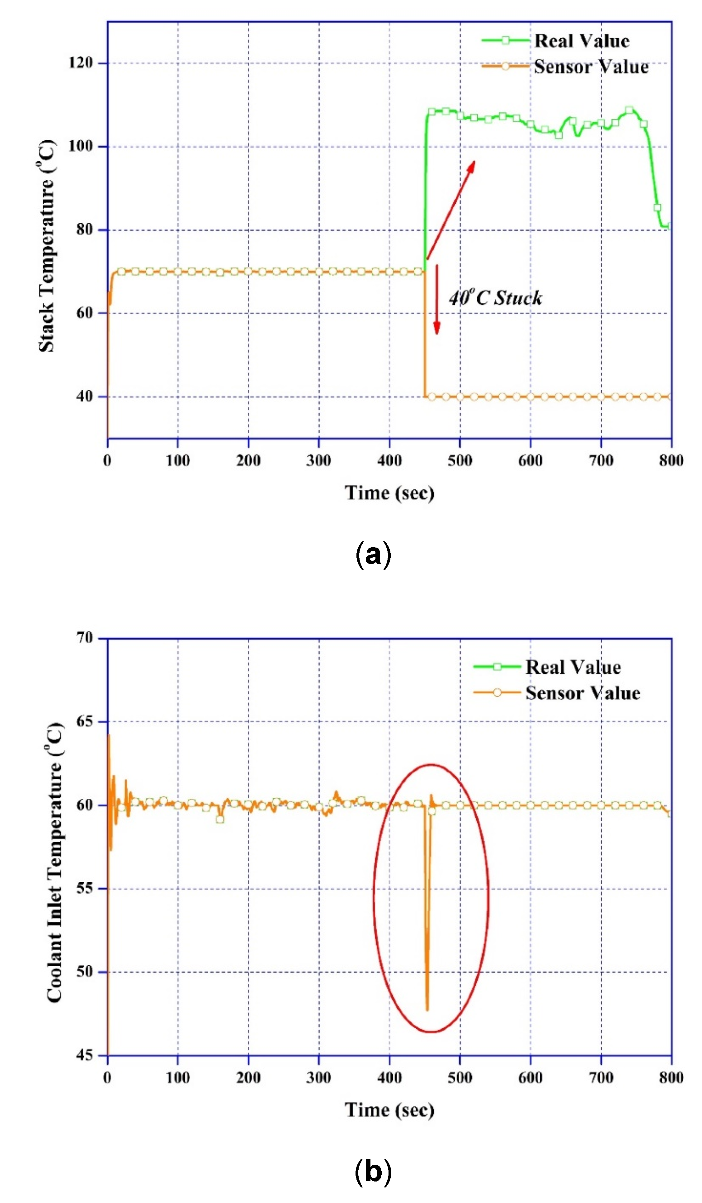
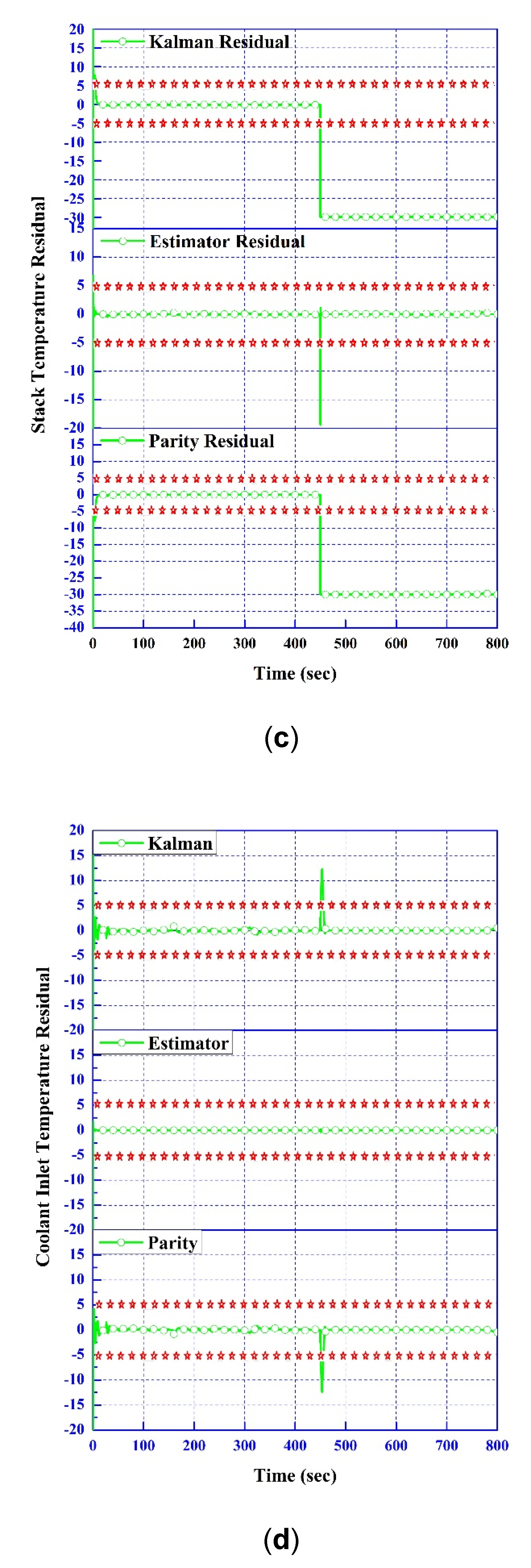
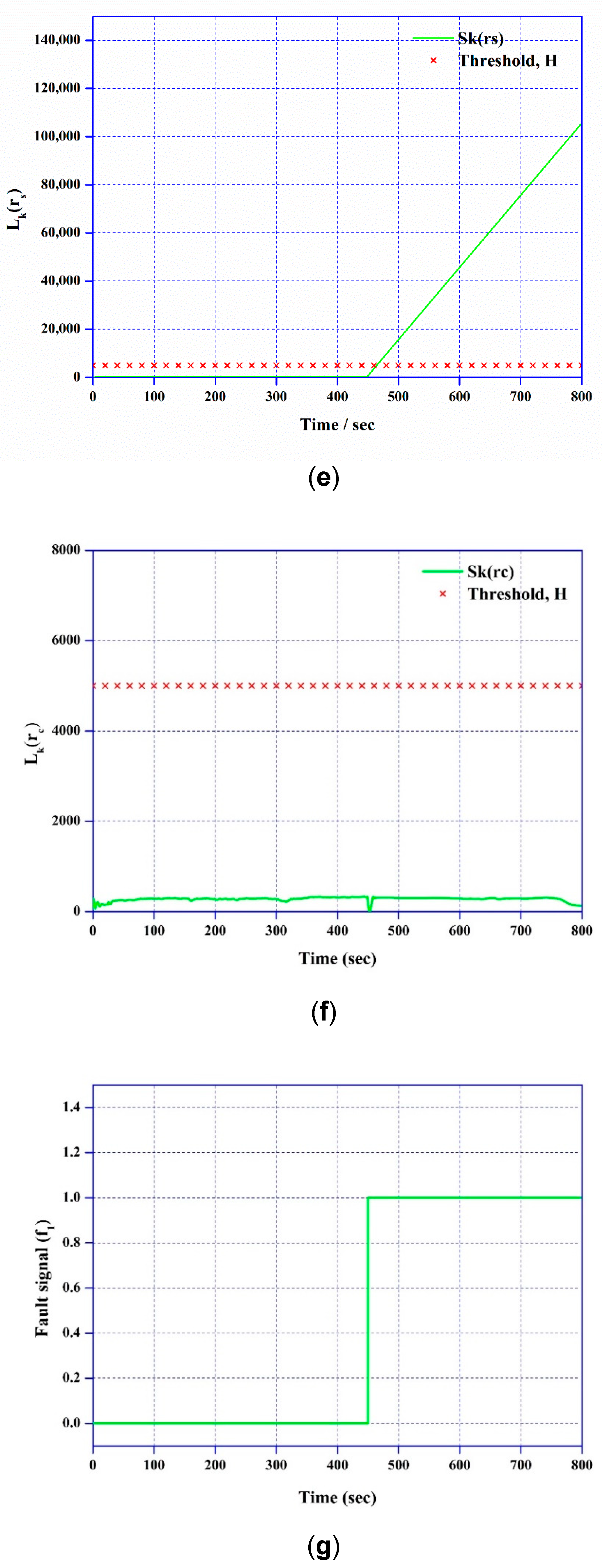
4.3.1. Fault Detection and Isolation with Stack Temperature Sensor Stuck

A test of stack temperature sensor fault f₁ stuck at 40 °C after injection at time 450 s is shown in Figure 7, with the actual stack and coolant inlet temperature sensor outputs, residuals, and corresponding detection and isolation results that were recorded. First, the real stack temperature and real coolant inlet temperature were determined; it can be observed from Figure 7a,b that the real stack temperature value increased after 450 s, while the real coolant inlet temperature value was maintained at 60 °C despite the occurrence of downshoot at 450 s. When the stack sensor stuck fault occurs, the water pump does not operate because the stack temperature sensor output is lower than the desired temperature control value (70 °C). This explains why the real stack temperature increased.

It can be seen in Figure 7c that the responses of the parity and Kalman filter residuals of the stack temperature to this fault are highly sensitive, whereas the estimator residual responds only slightly to this fault. Moreover, it can be seen from Figure 7d that the responses of the parity and Kalman Filter residuals of the coolant inlet temperature to these faults are slight. On the other hand, the estimator residual does not respond to this fault. According to the residual characteristics listed in Table 2, fault f₁ will occur when the stack temperature sensor responds to this fault. The CUSUM test result L_k of the residual confirms the presence of this fault, as shown in Figure 7e,f. This is because the stack CUSUM value, L_k(r(s)), exceeds the allowed threshold value at the time 450 s. On the other hand, the coolant threshold H does not cross the allowed threshold value. Therefore, there is no sensor fault in the coolant inlet temperature sensor. Finally, the isolated fault f₁ is shown in Figure 7g.

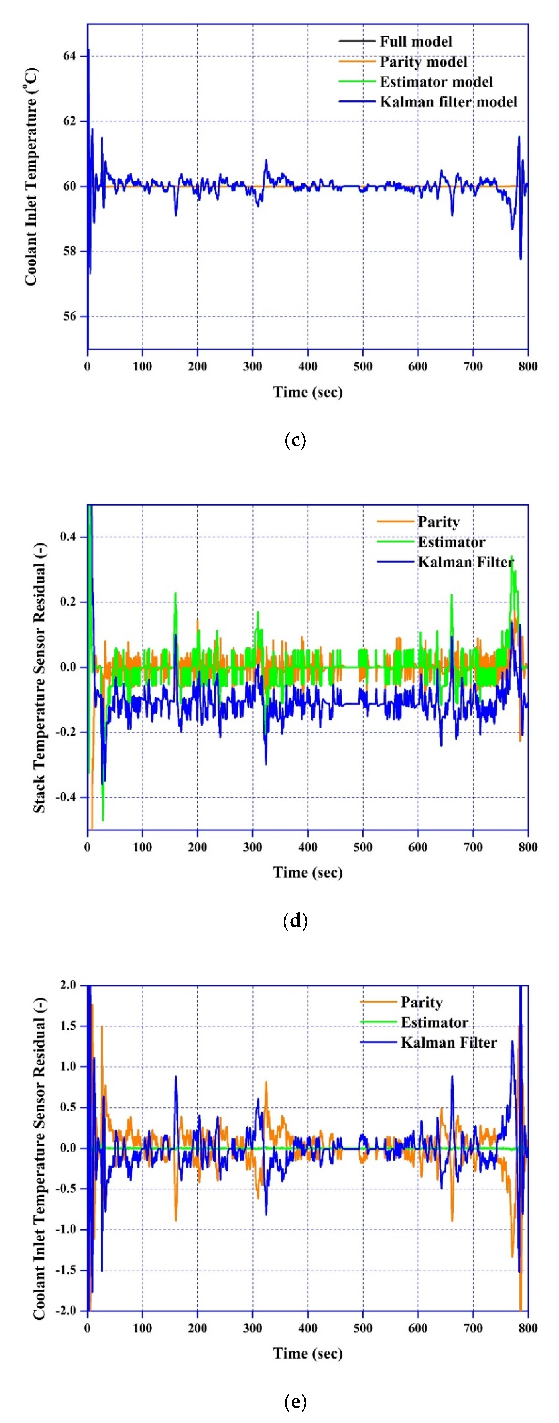
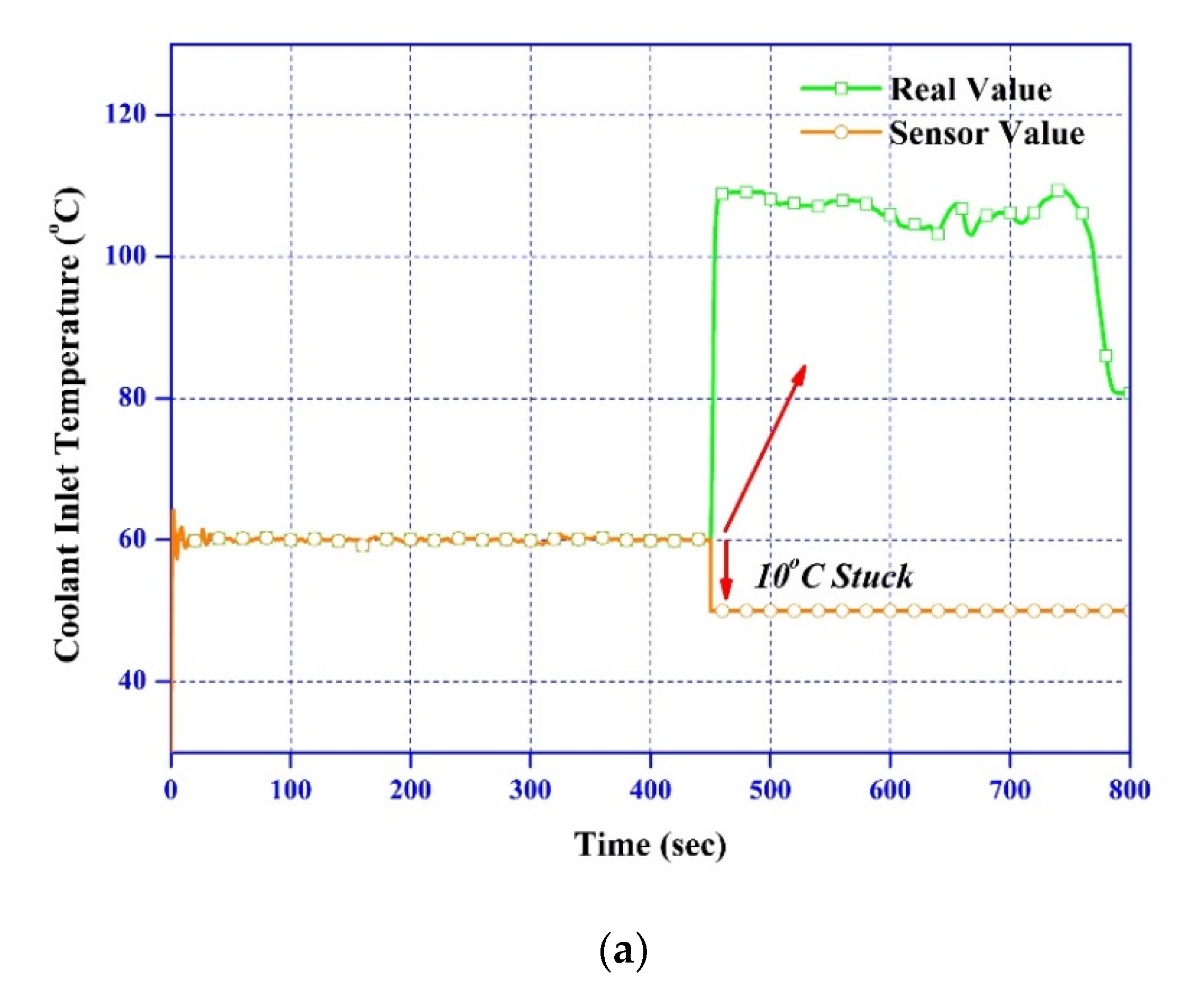
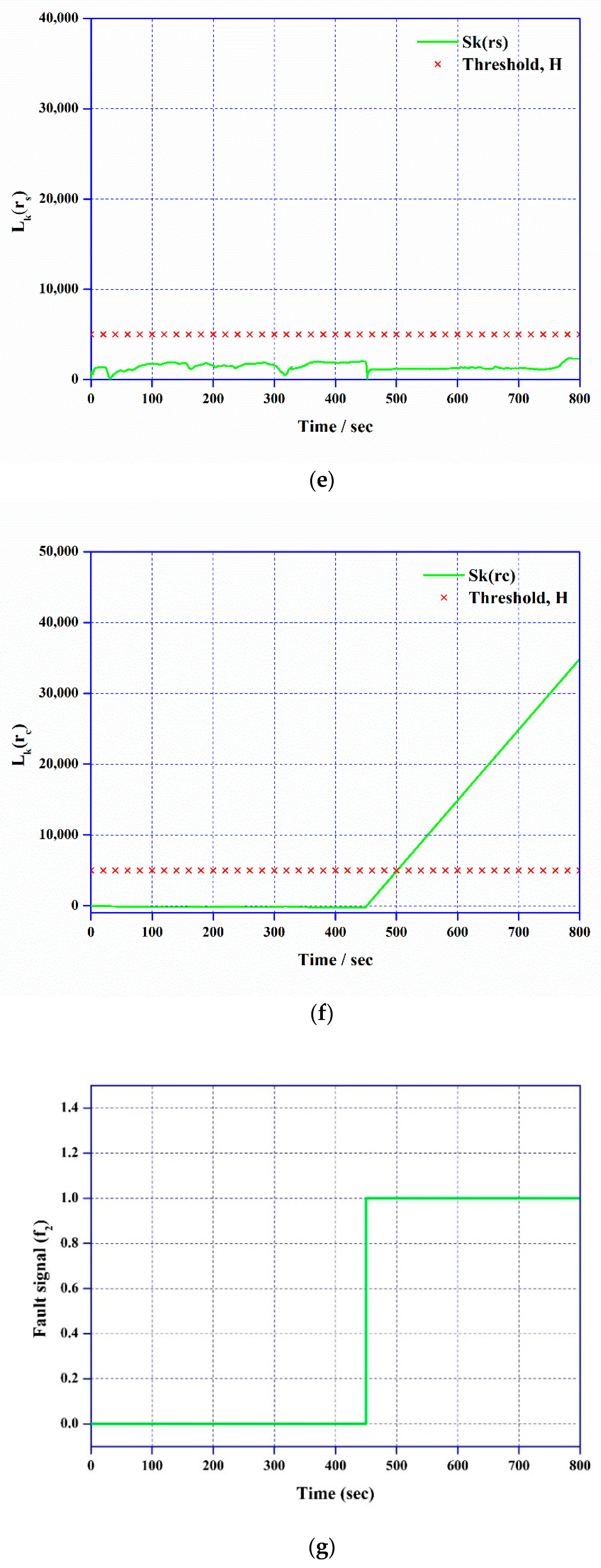
4.3.2. Fault Detection and Isolation with Coolant Inlet Temperature Sensor Stuck

Similarly, coolant inlet temperature sensor detection and isolation in the case of a coolant inlet sensor stuck fault was evaluated under HWFET cycles based on the current density. Taking a fault resulting from the coolant inlet temperature sensor being stuck at 10 °C upon injection into the coolant inlet at time 450 s, the detection and isolation results are plotted in Figure 8. Figure 8a,b shows the value measured by the temperature sensor and the real temperature value of the stack and coolant inlet, respectively. Figure 8a,b indicates that the real stack temperature increased after 450 s, because the radiator fan stopped. Because the real coolant inlet temperature increases, the stack temperature increases continuously, even though the water pump speed increases. Thus, a faulty coolant inlet temperature sensor can cause critical damage to the fuel cell stack.

In addition, Figure 8c,d shows the generated residual values r obtained with the three respective methods. The figure shows that the parity and the Kalman filter residuals exhibit a shift drop after 450 s, after which the value is maintained until the end of the cycle. On the other hand, the estimator residual undergoes a distinct drop at approximately 450 s; then, the residual immediately becomes similar to what it was before fault injection. Therefore, the results of the CUSUM test, shown in Figure 8e,f, show that the threshold was exceeded at 450 s, indicating a fault in the coolant inlet temperature sensor. Consequently, the CUSUM result L_k of the residual r_i confirms this result as the threshold H is crossed at 450 s, as shown in Figure 8e. That is why even if the residuals in the stack are zero, the actual and sensor values are the same. This means that the stack sensor has not failed.

The isolated fault signal of the temperature sensor is plotted in Figure 8g.

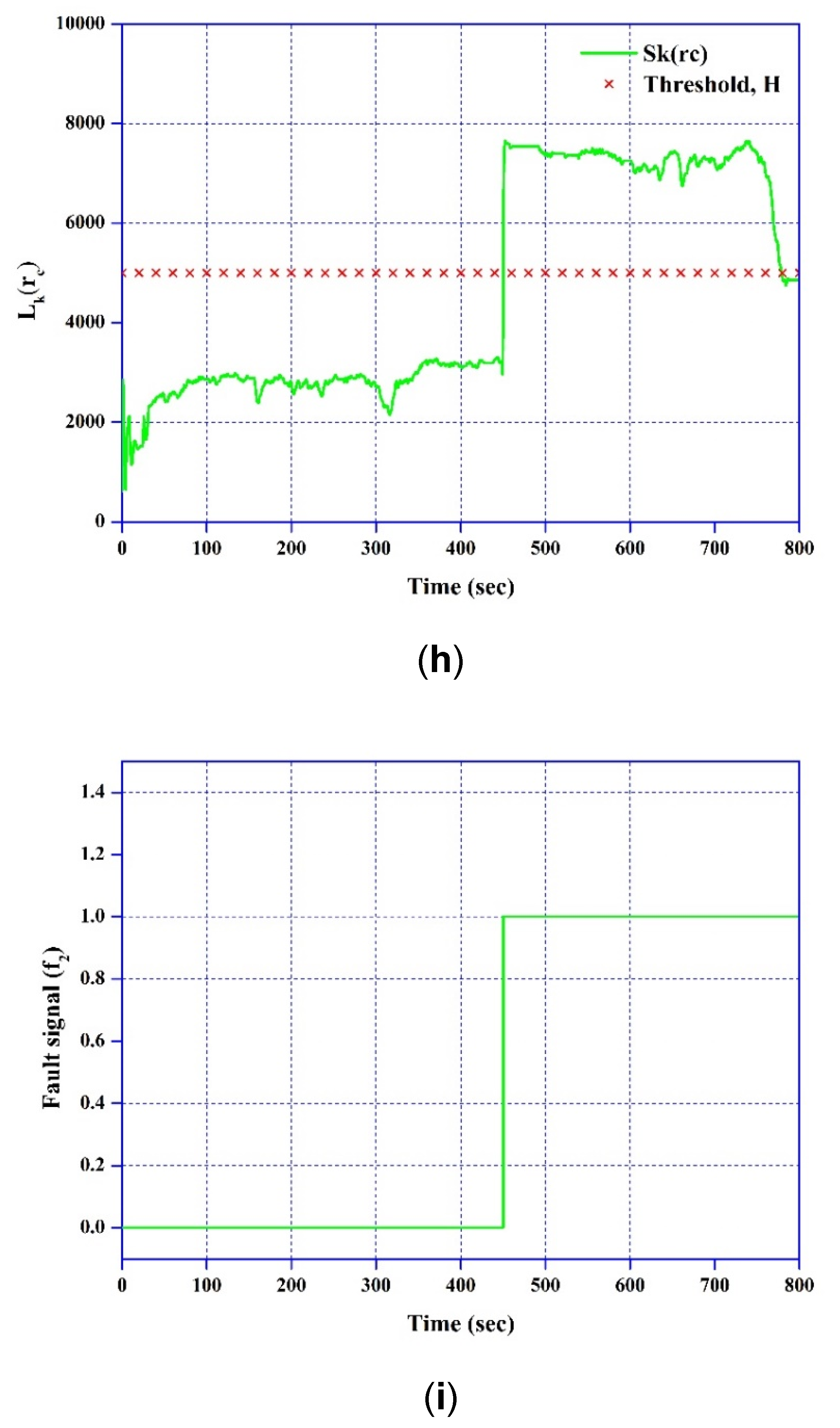
4.3.3. Fault Detection and Isolation by Scaling of Coolant Inlet Temperature Sensor

This section presents an evaluation of the coolant inlet temperature sensor. The sensor experiences 20% off-scaling in terms of degrees of temperature at 450 s. The detection and isolation results are plotted in Figure 9. Figure 9a,b shows the temperature sensor measurements and the real temperature values of the stack and coolant inlet, respectively. From the temperature screening results, it can be seen that the value of the stack temperature sensor is the same as the real temperature. On the other hand, the real value of the coolant inlet temperature increased when a scaling fault occurred at the coolant inlet temperature sensor. However, the coolant inlet temperature was maintained by the radiator fan controller, even during sensor faults. Figure 9c,d shows the speed of the water pump and the radiator fan. Under normal conditions, the motor speed of the radiator fan decreased from its operating speed after 450 s. This is why the motor controller detected the scaled value of the coolant inlet temperature from the sensor. Hence, the controller reduced the motor speed because of the low heat capacity in the cooling water and, consequently, the real temperature of the coolant inlet increased. This, in turn, caused the water pump motor speed to increase in response to the high temperature at the coolant inlet.

It can be seen from Figure 9e,f that the parity and Kalman filter residuals of the stack responded to this fault in the form of a peak, in contrast to the estimator residual, which responded only slightly. Furthermore, Figure 9e shows that the residuals of the stack temperature hardly responded to this fault. Especially, the maximum peer value cannot be exceeded in the case of the three residuals. That is why the temperature measured by the stack temperature sensor recovered immediately because of the water pump. On the other hand, the estimator residual of the coolant inlet temperature did not respond to this fault, whereas the parity and the Kalman filter residuals exceeded the threshold value. According to the residual characteristics in Table 2, fault f₂ will be detected when the coolant inlet temperature sensor responds to this fault. Unlike the stuck case, the residuals of the stack and the coolant inlet exist in the form of a peak. This is why the controllers of the water pump and the radiator fan continue operating in the case of a sensor scaling fault. The CUSUM test results indicate that a fault occurred in the coolant inlet temperature sensor, as shown Figure 9g,h. The coolant inlet temperature L_k(r(c)) crossed the allowed threshold value at 450 s, and L_k(r(c)) was maintained. On the other hand, the coolant threshold did not cross the specified threshold value. Thus, a sensor fault in the coolant inlet temperature sensor was indicated. Finally, the isolated fault signal f2 is shown in Figure 9i.

5. Conclusions

To evaluate three methods of fault detection and isolation under a real driving load profile, a parity equation, a state observer, and a Kalman filter method have been designed. Also, this paper presents a comparison of three residuals derived from the parity equation, state observer, and Kalman filter, as well as a method for detection and isolation of faults in a cooling system temperature sensor in a lumped fuel cell system.

• The parity equation, state observer, and Kalman filter methods for fault detection were developed in this study. The temperature outputs of a nonlinear fuel cell system were monitored; then, estimated linear model outputs were compared with those of the nonlinear fuel cell system to generate a residual. The generated residuals were evaluated by the CUSUM method to identify the presence of a sensor fault.
• The fuel cell was operated under normal conditions, with a load step, to determine the allowed residual threshold. The HWFET driving cycle was used to evaluate the proposed fault diagnosis methods under real vehicle operating conditions.
• The proposed FDI schemes can effectively detect faults in the stack temperature sensor and coolant inlet temperature sensor. In addition, CUSUM can effectively identify locations of temperature irregularity.

References

1. Da Fonseca, R.; Bideaux, E.; Gerard, M.; Jeanneret, B.; Desbois-Renaudin, M.; Sari, A. Control of PEMFC system air group using differential flatness approach: Validation by a dynamic fuel cell system model. Appl. Energy 2014, 113, 219–229. [Google Scholar] [CrossRef]
2. Jinlong, L.; Tongxiang, L.; Hongyun, L. Effect of grain refinement and electrochemical nitridation on corrosion resistance of the 316L stainless steel for bipolar plates in PEMFCs environment. J. Power Sources 2015, 293, 692–697. [Google Scholar] [CrossRef]
3. Mousa, G.; Golnaraghi, F.; DeVaal, J.; Young, A. Detecting proton exchange membrane fuel cell hydrogen leak using electrochemical impedance spectroscopy method. J. Power Sources 2014, 246, 110–116. [Google Scholar] [CrossRef]
4. Xu, L.; Mueller, C.D.; Li, J.; Ouyang, M.; Hu, Z. Multi-objective component sizing based on optimal energy management strategy of fuel cell electric vehicles. Appl. Energy 2015, 157, 664–674. [Google Scholar] [CrossRef]
5. Feroldi, D.; Carignano, M. Sizing for fuel cell/supercapacitor hybrid vehicles based on stochastic driving cycles. Appl. Energy 2016, 183, 645–658. [Google Scholar] [CrossRef]
6. Bizon, N. On tracking robustness in adaptive extremum seeking control of the fuel cell power plants. Appl. Energy 2010, 87, 3115–3130. [Google Scholar] [CrossRef]
7. Simons, A.; Bauer, C. A life-cycle perspective on automotive fuel cells. Appl. Energy 2015, 157, 884–896. [Google Scholar] [CrossRef]
8. Xuewei, P.; Rathore, A.K. Novel Bidirectional Snubberless Naturally Commutated Soft-Switching Current-Fed Full-Bridge Isolated DC/DC Converter for Fuel Cell Vehicles. IEEE Trans. Ind. Electron. 2013, 61, 2307–2315. [Google Scholar] [CrossRef]
9. Yuan, X.-Z.; Li, H.; Zhang, S.; Martin, J.; Wang, H. A review of polymer electrolyte membrane fuel cell durability test protocols. J. Power Sources 2011, 196, 9107–9116. [Google Scholar] [CrossRef] [Green Version]
10. Wang, Y.; Chen, K.S.; Mishler, J.; Cho, S.C.; Adroher, X.C. A review of polymer electrolyte membrane fuel cells: Technology, applications, and needs on fundamental research. Appl. Energy 2011, 88, 981–1007. [Google Scholar] [CrossRef] [Green Version]
11. Pei, P.; Li, Y.; Xu, H.; Wu, Z. A review on water fault diagnosis of PEMFC associated with the pressure drop. Appl. Energy 2016, 173, 366–385. [Google Scholar] [CrossRef]
12. Shao, M.; Zhu, X.-J.; Cao, H.-F.; Shen, H.-F. An artificial neural network ensemble method for fault diagnosis of proton exchange membrane fuel cell system. Energy 2014, 67, 268–275. [Google Scholar] [CrossRef]
13. Pahon, E.; Steiner, N.Y.; Jemei, S.; Hissel, D.; Mocoteguy, P. A signal-based method for fast PEMFC diagnosis. Appl. Energy 2016, 165, 748–758. [Google Scholar] [CrossRef]
14. Escobet, T.; Feroldi, D.; De Lira, S.; Puig, V.; Quevedo, J.; Riera, J.; Serra, M. Model-based fault diagnosis in PEM fuel cell systems. J. Power Sources 2009, 192, 216–223. [Google Scholar] [CrossRef] [Green Version]
15. Li, Z.; Outbib, R.; Giurgea, S.; Hissel, D.; Li, Y. Fault detection and isolation for Polymer Electrolyte Membrane Fuel Cell systems by analyzing cell voltage generated space. Appl. Energy 2015, 148, 260–272. [Google Scholar] [CrossRef]
16. Puig, V.; Feroldi, D.; Serra, M.; Quevedo, J.; Riera, J. Fault-Tolerant MPC Control of PEM Fuel Cells. IFAC Proc. Vol. 2008, 41, 11112–11117. [Google Scholar] [CrossRef]
17. Mocoteguy, P.; Ludwig, B.; Steiner, N.Y. Application of current steps and design of experiments methodology to the detection of water management faults in a proton exchange membrane fuel cell stack. J. Power Sources 2016, 303, 126–136. [Google Scholar] [CrossRef]
18. Polverino, P.; Frisk, E.; Jung, D.; Krysander, M.; Pianese, C. Model-based diagnosis through Structural Analysis and Causal Computation for automotive Polymer Electrolyte Membrane Fuel Cell systems. J. Power Sources 2017, 357, 26–40. [Google Scholar] [CrossRef] [Green Version]
19. Rosich, A.; Sarrate, R.; Nejjari, F. On-line model-based fault detection and isolation for PEM fuel cell stack systems. Appl. Math. Model. 2014, 38, 2744–2757. [Google Scholar] [CrossRef]
20. Zhang, L.; Huang, A.Q. Model-based fault detection of hybrid fuel cell and photovoltaic direct current power sources. J. Power Sources 2011, 196, 5197–5204. [Google Scholar] [CrossRef]
21. De Lira, S.; Puig, V.; Quevedo, J.; Husar, A. LPV observer design for PEM fuel cell system: Application to fault detection. J. Power Sources 2011, 196, 4298–4305. [Google Scholar] [CrossRef] [Green Version]
22. Kamal, M.; Yu, D.; Yu, D. Fault detection and isolation for PEM fuel cell stack with independent RBF model. Eng. Appl. Artif. Intell. 2014, 28, 52–63. [Google Scholar] [CrossRef]
23. Yu, S.; Han, J.; Lee, S.M.; Lee, Y.D.; Ahn, K.Y. A Dynamic Model of PEMFC System for the Simulation of Residential Power Generation. J. Fuel Cell Sci. Technol. 2010, 7, 061009. [Google Scholar] [CrossRef]
24. Han, J.; Yu, S.; Yi, S. Advanced thermal management of automotive fuel cells using a model reference adaptive control algorithm. Int. J. Hydrogen Energy 2017, 42, 4328–4341. [Google Scholar] [CrossRef]
25. Han, J.; Yu, S.; Yi, S. Adaptive control for robust air flow management in an automotive fuel cell system. Appl. Energy 2017, 190, 73–83. [Google Scholar] [CrossRef]
26. Han, J.; Park, J.; Yu, S. Control strategy of cooling system for the optimization of parasitic power of automotive fuel cell system. Int. J. Hydrogen Energy 2015, 40, 13549–13557. [Google Scholar] [CrossRef]
27. Franklin, G.F.; Powell, J.D.; Emami-Naeini, A. Feedback Control of Dynamic Systems, 6th ed.; Pearson: New York, NY, USA, 2010; pp. 63–68. [Google Scholar]
28. Amphlett, J.C.; Baumert, R.M.; Mann, R.F.; Peppley, B.A.; Roberge, P.R.; Harris, T.J. Performance modeling of the Ballard Mark IV solid polymer electrolyte fuel cell I. Mechanistic model development. J. Electrochem. Soc. 1995, 142, 1–8. [Google Scholar] [CrossRef]
29. Mammar, K.; Chaker, A. Modelling and fuzzy logic control of PEM fuel cell system power generation for residential application. J. Electr. Electron. Eng. 2009, 9, 1073–1081. [Google Scholar]
30. Chen, C.-T. Linear System Theory and Design -3/E; OXFORD: London, UK, 2004. [Google Scholar]
31. Martinez-Guerra, R.; Mata-Machuca, J.L. Fault Detection and Diagnosis in Nonlinear Systems; Springer: Berlin/Heidelberg, Germany, 2014. [Google Scholar]
Figure 1. Schematic diagram of whole fuel cell system.
Processes 08 01115 g001
Figure 2. Characteristic performance of air blower with respect to motor speed (a)—performance P-Q curve, (b)—blower efficiency.
Processes 08 01115 g002
Figure 3. Dynamic thermal management system for sensor fault diagnosis.
Processes 08 01115 g003
Figure 4. Schematic diagram of proposed model-based fault detection for cooling system sensor ((a) Parity method, (b) State observer and Kaman filter method).
Processes 08 01115 g004
Figure 5. Unit cell test bench and results of validation of I-V curve ((a)—unit cell test bench, (b)—results of validation of I-V curve with experimental data).
Processes 08 01115 g005aProcesses 08 01115 g005b
Figure 6. Highway Fuel Economy Test (HWFET) test results in normal condition. ((a)—Current density profiles, (b)—Stack temperature variation, (c)—Coolant inlet temperature variation, (d)—Stack temperature sensor residual, (e)—Coolant inlet temperature sensor residual).
Processes 08 01115 g006aProcesses 08 01115 g006b
Figure 7. Sensor measurements, residuals and detection results in the stack stuck fault of HWFET driving cycle ((a)—stack temperature values, (b)—Coolant inlet temperature value, (c)—residual from the stack sensor, (d)—residual from the coolant inlet temperature, (e)—Cumulative sum (CUSUM) result from the stack temperature sensor, (f)—CUSUM result from the coolant inlet temperature sensor, (g)—isolated temperature sensor fault f1 signal.).
Processes 08 01115 g007aProcesses 08 01115 g007bProcesses 08 01115 g007c
Figure 8. Sensor measurements, residuals, and detection results in coolant inlet stuck fault of HWFET driving cycle ((a)—Coolant inlet temperature value, (b)—Stack temperature value, (c)—residual from stack sensor, (d)—Residual from coolant inlet temperature, (e)—CUSUM result from stack temperature sensor, (f)—CUSUM result from coolant inlet temperature sensor, (g)—Isolated temperature sensor fault f2 signal).
Processes 08 01115 g008aProcesses 08 01115 g008bProcesses 08 01115 g008c
Figure 9. Sensor measurements, residuals, and detection results in coolant inlet scaling fault of HWFET driving cycle ((a)—Stack temperature values, (b)—Coolant inlet temperature value, (c)—Water pump motor speed, (d)—Radiator fan motor speed (e)—Residual from stack sensor, (f)—Residual from coolant inlet temperature, (g)—CUSUM result from stack temperature sensor, (h)—CUSUM result from coolant inlet temperature sensor, (i)—Isolated temperature sensor fault f2 signal).
Processes 08 01115 g009aProcesses 08 01115 g009bProcesses 08 01115 g009cProcesses 08 01115 g009d