Abstract
Fault detection is one of the key steps in Fault Detection and Isolation (FDI) and, therefore, critical for subsequent prognosis or implementation of Fault Tolerant Control (FTC). It is, therefore, advisable to utilize detection algorithms which are quick and can detect the smallest faults. Model-based detection methods satisfy both these criteria and should be preferred. However, a big limitation for model-based methods is that they require the accurate value of the component parameters, which is difficult to obtain in real situations. This limits the accuracy of model-based methods. This paper proposes a new method for fault detection using Energy Activity (EA) which can detect minute levels of fault in systems with high component uncertainty. Different forms of EA are developed for use as an FDI metric. The proposed forms are simulated using a two-tank system under various types of faults. The results are compared with each other and with the traditional model-based FDI method using Analytical Redundancy Relations (ARRs). The simulations are performed considering model uncertainties to check the inherent performance of the methods. From initial simulations, it is established that the integral form of EA is most suited for fault detection. The integral for if EA is then tested using a real two-tank system considering both the model and measurement uncertainties.
1. Introduction
Accurate and timely detection of fault (i.e., a deviation of the system from its desired operating conditions) is the one of the key objectives of any Fault Diagnosis and Isolation (FDI) system. The FDI framework should be able to detect the fault at the earliest. An early detection of fault enables a wider variety of response actions for the fault. The post-fault detection decision depends on the Remaining Useful Life of the system [1]. Therefore, an early detection of faults can give more options for response for, e.g., implementing fault tolerant control or scheduling maintenance or immediate intervention. This can be a of great advantage if the system under consideration is critical to safety.
Fault detection and Isolation (FDI) methods can be categorized as Data-Driven or Model-Based. Data-driven approaches use statistical [2,3,4,5] or Artificial Intelligence [6,7,8] techniques to map the measure parameters to ideal working conditions. Any deviation of measured values from a set range indicates a fault. Data-driven techniques are very successful in industrial application and are very commonly used as there is no need for analytical models; however, there are certain limitations. The major limitation is that these techniques require a lot of data for system under faulty conditions for proper mapping. Allowing a system to remain in faulty state is not desired. A deep review of various methods of fault detection can be found in Reference [9].
Model-based approaches [10,11] use mathematical models derived from governing laws of physics. These approaches are preferred because they give a basic understanding about the functioning of the system and, hence, can be used with accuracy in any working conditions. The model can either be qualitative or quantitative [12]. Based on the the model, certain equations called residuals are generated, which can capture the operating state of various components of the system. One of the major limitation for model-based approach is that, many times, all the system component values are not known with high accuracy, which is a necessity for proper detection and decision.
This problem is solved by calculating suitable range for the residuals. The limits are calculated based on the uncertainty associated with a component [13]. Fault is detected when the residual deviates outside the prescribed limits. Sometimes, some components in the system have high uncertainty associated with them. This leads to a wide range of allowed value of residuals. In this case, it is possible that a smaller fault might not be able to cause a deviation in the residual high enough for fault detection, even if it occurs in a component known with high certainty. This leads to missed alarms in the faulty system. This situation can be of great concern, especially in systems critical to safety.
This need for improvement is recognized, and a lot of efforts have been made to reduce missed alarms. However, most of the work focuses on reducing uncertainty propagation and, therefore, work on reducing the allowable range for the residuals [14,15,16]. Many other solutions for fault detection require use of different mathematical techniques, such as maximum probability machine [17], optimization [18], and filters [19,20]. Methods specific to certain types of systems have also been suggested. For example, References [21,22] worked on fault detection specifically for Markov jump system. In addition, much focus has been laid on data fusion from a variety of instruments for fault detection [23,24,25,26].
However, very little work has been done on development on new forms of residuals for fault detection. In this paper, a new metric of fault detection is proposed that can detect small magnitude faults that are not detected by traditional fault detection methods due to high uncertainty in system information and measurements. The proposed metric has the following properties which make it a better choice for fault detection:
- 1.
- Energy-Based: The proposed metric is a parameter based on energy and has a physical significance. Therefore, it is easier to understand and better suited to multi-domain systems.
- 2.
- History: Most of the residuals used for fault detection are found using Analytical Redundancy Relations (ARR) and observers. These methods only use the instantaneous information about the system to detect fault. It is proposed that development of a metric which can use both the current and previous information about the state of the system can be a better solution to reduce missed alarms.
- 3.
- Isolation from uncertain components: The proposed metric depends only on various values detected using sensors and the component value of only the component for which it is calculated, whereas traditional methods use equations that depend on sensor values in conjunction with the component values of various components, including uncertain ones. The isolation of the metric from multiple uncertain component values reduces the propagated uncertainty.
The main contributions of this paper are as follows:
- 1.
- Novel fault detection methods using Energy Activity (EA) is developed. The proposed methods can accommodate model and measurement uncertainties.
- 2.
- The proposed methods are compared using simulations, with each other and with existing fault detection method, i.e., Analytical Redundancy Relations (ARRs).
- 3.
- Comparison is made on three types of faults, i.e., abrupt fault, intermittent fault, and incipient fault, of low magnitude.
- 4.
- The best performing method is validated on a real two-tank system under model and measurement uncertainties.
This paper is organized as follows. Section 1 introduces to the basic concepts, requirements, and challenges of accurate and rapid fault detection. Section 2 introduces to basic concept of bond graph modeling and establishes bond graph as a tool for fault detection. Section 3 describes the concept of Energy Activity in its various forms for use in fault detection. Section 4 describes the system used for simulation. Analytical Redundancy Relations are derived, and Energy Activity is also calculated for the system. In Section 5, the performance of fault detection methods from previous methods is compared and discussed. Section 6 deals with implementation of the best performing EA method on a real system. The paper concludes in Section 7.
2. Fault Detection Using Bond Graph
Bond graph [27,28] is a powerful tool for multi-physics dynamic modeling and based on energy exchange. Being a component-based technique, bond graphs can identify and model the individual components. This also allows easier subsystem visualization while modeling the dynamics, giving the user a better understanding of the results. This technique is based on the law of conservation of energy, thus using the time derivative of energy, i.e., power, to calculate the dynamics of the system. As law of conservation of energy concerns any kind of physical domain, bond graph technique as an unified and multi-physics (including thermal, mechanical, electrical, etc.) modeling tool is well suited for such task. Moreover, bond graph tool can be used not only for modeling but also for control and diagnosis analysis because of its causal and structural properties.
Power in any component can be measured as the product of an agent causing the change and the rate of observed change. In bond graph, these are called generalized effort e and generalized flow f, respectively. Effort and flow represent an intensive and derivative of extensive variable, respectively. Their product is the exchanged power. The components that make up a system can be either storing or dissipate energy. In bond graph technique, components that store generalized kinetic energy are described as Inertia (I) elements, components that store generalized potential energy are described as Compliance (C) elements, and the components that dissipate energy are described as Resistance (R) elements. The system might also have components that convert or morph the energy. These elements can be described using two components, i.e., Transformers () and Gyrators (). The various components interact among each other and the system, through either a 1 or 0 junction. Components joined through a common 1 junction have equal generalized flow; on the other hand, those joined through common 0 junction have a equal generalized effort. Energy can be provided to the system by either a flow source () or an effort source ().
As discussed earlier, managing individual components using bond graphs is easier. As, the 0 and 1 junctions impose a structural condition on the the various components of the system, usually representing a physical phenomenon, such as Kirchhoff’s law, bond graph is suited for model-based detection. Hence, the structural nature of bond graph modeling has been successfully used for fault diagnosis [29].
A fault in a bond graph is represented as a deviation from nominal value (nominal operating mode) of its parameter represented by bond graph element (R, C, I, Tf, and GY). Depending upon their nature, the faults can be categorized in three types [30].
- Abrupt Fault: This fault occurs in a step-wise fashion and stays present. This fault is usually observed in components which cannot vary continuously but in discrete steps.
- Intermittent Fault: This fault occurs and disappears suddenly. The fault magnitude and duration do not have a fixed pattern and vary randomly. This type of fault is usually caused due to environmental interference.
- Incipient Fault: This fault causes a gradual drift in the component value. This fault occurs due to gradual degradation of the system over time.
A popular method for fault detection using bond graphs requires the generation of ARRs. ARRs in bond graphs are calculated by creating the system in preferred differential causality. The system measurements from the real system are imposed (called duality of sensors). The structural relationship at the junction is then monitored. The equation for checking the structure is called an ARR. To accommodate known uncertainty in the model, LFT-bond graph is usually used [13]. The known uncertainty is added to the component input using a virtual detector. This allows the calculation of the bounds of ARR due to uncertainty.
3. Energy Activity for Fault Detection
All the components, in a dynamic system, irrespective of their domain, interact with each other through energy. Certain components can either absorb or release the energy during the different phases of their interaction. There are also other components which can just dissipate the energy out of the system. The amount of energy that these components interact with depends on the numeric values of the different components of the system. When a component is in a faulty state, its numeric component value and, hence, the energy interaction for that of the system component changes. As energy can neither be created or be destroyed, the complete system experiences a redistribution of energy. Monitoring this energy interaction in the various components of the system can help in fault detection. Bond graph, being a component-based approach, is suited for study of such interaction. For the work presented in this paper, energy interaction of the components of the system is studied using Energy Activity.
Historically, the concept of EA was introduced as a tool for physical model reduction [31]. EA is the total energy interaction (storage and release) that a component has with the system over a specified time period. The primary difference between energy and energy activity is that, while the energy state of a component can increase or decrease, the energy activity of the component always increases. The equations for energy and energy activity are given by Equations (1) and (2), respectively. The difference between the two can be understood using Figure 1. Figure 1b shows the energy and EA associated for any system component undergoing a variation of power shown in Figure 1a. It should also be noted that EA of a component can never decrease with time.
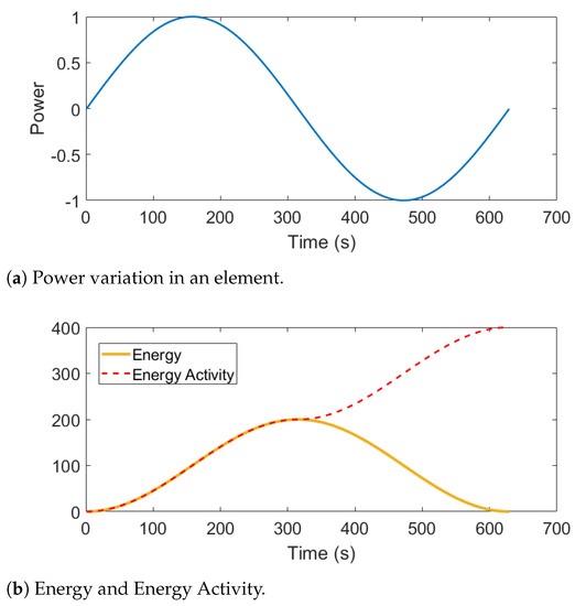
Figure 1.
Difference between energy and Energy Activity.
In the context of bond graph, power associated in any element can be defined as the product of the generalized flow and generalized effort. EA is, therefore, defined using Equations (3) and (4).
In Equation (3), e and f are the generalized effort and flow, respectively. In Equation (4), S is the signal input from the system to the component. According to the causality (derivative or integral) associated with the component, S represents the flow or effort input signal. Function g is the Constitutive Relationship (CR), i.e., Equation (4) expresses the relation between the component input and output. It corresponds to the physical law applied by the component. It uses the numeric component value .
The function g for energy storing elements (I and C) can be in either integral or differential form. The form used for fault detection depends on which power variable (e or f) is known. The equations for g for C and I elements in both integral and differential form are given by Equations (5) and (6), respectively.
The function g for energy dissipating elements (R) is algebraic; however, the form used depends on the power variable known. Both the forms are given in Equation (7).
The above can be explained with the following example. Figure 2 illustrates a simple RIC circuit. The dynamic model for the system can be either in preferred integral causality (Figure 3a) or in preferred differential causality (Figure 3b). As the components of the circuit are in series, i.e., they undergo equal flow (current), therefore, in the bond graph model, the components are attached to a 1-junction. A 1-junction can only have one component that governs the flow. Hence, this flow is governed by I when using preferred integral causality and by C when using the preferred differential causality. For model in preferred integral causality, the generalized effort and generalized flow are given in Table 1. Similarly, for a model in preferred differential causality, the generalized effort and generalized flow are given in Table 2.
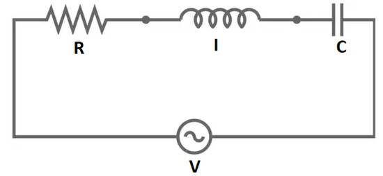
Figure 2.
Simple RIC circuit.
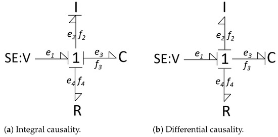
Figure 3.
Bond graph models of RIC circuit.

Table 1.
Effort and flow calculation in preferred integral causality.
Table 2.
Effort and flow calculation in preferred differential causality.
Consider the I element in preferred integral causality for calculation of EA. The input to the element is generalized effort; therefore, S for I element in integral causality is the generalized flow e. Hence, the for the element in its current form is the integral of the S (). In addition, in this case, is given as . For the same element (I) in preferred differential causality, S is the generalized flow f, is given as time derivative if S, i.e., , and is given as I.
Energy Activity Index (EAI) [31] of any component, calculated during a time interval, is the fraction of the energy activity of that component, in the total energy activity of the system during the same time. Hence, energy activity index analysis gives us the relative comparison of the activity of different components in the system. The expression used for the calculation of energy activity index of component i in a system containing n components is given by Equation (8). EAI has been developed for model reduction [31], control [32], fault detection [33], and integrated diagnosis and prognosis [34] of systems.
For using Energy Activity as a metric for fault detection, the measured EA must be compared to the Energy Activity calculated from an ideal system simulation. The deviation of calculated energy activity from simulated energy activity indicates a fault. However, the simulated model must accommodate the uncertainty in various elements of the system. Therefore, the simulated system should give a range of Energy Activity instead of a precise value.
The method can be understood using Figure 4. A virtual system is simulated in parallel to the real system. Virtual measurements are made corresponding to the actual measurements of the real system. The information from real sensors is used to calculate the real EA of the system, and that from virtual systems is used to calculate the virtual EA. The uncertainty in system and measurement are accommodated in the virtual EA, and an envelope for virtual EA is obtained.
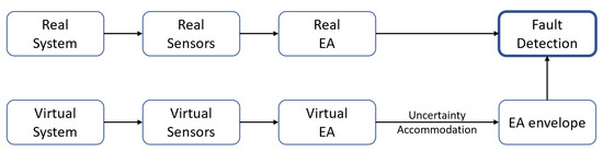
Figure 4.
Schematic of fault detection using Energy Activity.
The range of Energy Activity is calculated using Interval Extension Function (IEF). Under nominal behavior, an envelope around a calculated quantity can be defined by the range of the quantity calculated using IEF [14]. The bounds are, therefore, generated by solving the system under IEF.
For IEFs, the variables in the equation are replaced be an interval range. Therefore, the result is a range instead of a single fixed quantity. This can be used for accommodation of uncertainty in fault analysis [35,36]. The equations are then solved using the principles of interval arithmetic [37,38]. Any variable x in an equation with minimum possible value and maximum possible value is written as:
For the bond graph framework, EA can be calculated by creating the interval bond graph [39]. Consider an uncertain R-element in resistive causality. The constitutive relationship for the element is given by Equation (10), where e is the generalize effort, f is the generalized flow, and R is the numeric component value of the element.
The natural interval extension of the above can be derived as shown in Equation (11).
where is the nominal component effort, and is the uncertain component of effort.
Therefore, the simulated EA for any component can be solved as
where is the set of all the components in the system, and is the component for which EA is being calculated.
Energy Activity calculated using CR in differential form captures the history of how fast the component signal has changed. On the other hand, EA calculated using integral form captures the history total change in the component signal. This situation is analogous to control systems which use PD controllers which are based on rate of error to generate the control signal and PI controllers which are based on total error to generate the control signal. In control systems, PI and PD controllers led to the development of PID controllers. Similarly, the logical step in fault detection should also be to develop an EA metric which has both differential and integral components. This is achieved adding both the differential and integral forms of EA. From here on, the EA metric containing both the differential and integral form will be referred to as dual-EA. The equations representing the differential, integral and dual-EA are given by Equations (13)–(15), respectively. The variables and in Equation (15) are the gains associated with integral and differential component of the equation.
The following assumptions are considered for using the proposed method:
- 1.
- Only one component can undergo a fault at a time.
- 2.
- The noise to signal ratio is small known in priory.
- 3.
- All the components of dynamic model are recognized, i.e., all the components adding to the dynamics of the system are known and have been used in the model.
- 4.
- Fault occurs in the system components and not in the detectors.
At this point, it is important to understand the difference between the working of the ARR method and the proposed method. The ARR method identifies the structural relationship imposed by the model, utilizing the measured outputs of the system as inputs for the bond graph model in preferred differential causality. On the other hand, the proposed method checks for change in EA in various components compared to an ideal (fault-free) system. Therefore, the ARR method checks for deviation of imposed relationship among the measured values, but the proposed method checks for EA deviation against an ideal system.
Any fault, in any component of the system, leads to a deviation in all the measured values. Therefore, any fault in the system is captured by all the EAs calculated using the proposed method. Hence, fault detection can be done by calculating EA at any component of the system. The choice of the component to be used for fault detection is made using Energy Activity Index. EAI for all the components in ideal condition is checked. The element with the highest EAI is selected for fault detection. This is because the element with highest EAI is the most active component in the system; hence, a redistribution will have the highest effect on this component. In addition, due to the non-reducing nature of EA, a higher magnitude of EA makes it more robust to measurement noise.
The sequence of steps in order to implement the proposed method for fault detection are as follows:
- 1.
- Define the dynamic model of the system (preferably using bond graph) and find the generalized flow and generalized effort for individual components.
- 2.
- For each component, determine the equation for the EA calculation in differential and integral form.
- 3.
- Calculate the EAI for all the individual components to determine the more appropriate component for fault detection.
- 4.
- Calculate the residual in real time as:
4. System Simulation
The Energy Activity forms discussed in the previous section are simulated on a two-tank hydraulic test benchmark system. The fault detection performance of the proposed methods are also compared with each other and with residuals generated using ARRs. The schematic diagram of the system is represented by Figure 5. The system consists of two tanks joined to each other through a valve 1. Valve 2 is placed between tank 2 and the outlet. Continuous and constant fluid input is maintained using a fluid inlet pump (). The flow rate through valve 1 (), and flow rate through valve 1 (), is measured using sensors. The diameter of tanks are known; hence, compliance of tank 1 () and tank 2 () is known.
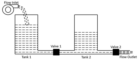
Figure 5.
Schematic diagram of a two-tank system.
As discussed earlier, any physical system has certain components in which physical parameters are not known with high accuracy. However, the uncertainty related to these components can be approximated. In the current system, the flow coefficient for valves 1 and 2 are not known with high accuracy. However, the flow coefficients have an assumed value of and , respectively, with an uncertainty of each. The parameters for the remaining components of the system are known with accuracy. The system parameters used for simulation are given in Table 3.
Table 3.
System parameters.
The system bond graphs in integral and differential form, for the simulated system is shown in Figure 6a,b, respectively. The generalized flow in hydraulic system represents the volume flow rate of the fluid, and the generalized effort represents pressure. For a system in the integral form, the system equations are solved in the integral form; hence, flow is imposed on the tanks, and effort is calculated. On the contrary, for system in differential form, the system equations are generated in the differential form; therefore, effort is imposed, and flow is calculated.
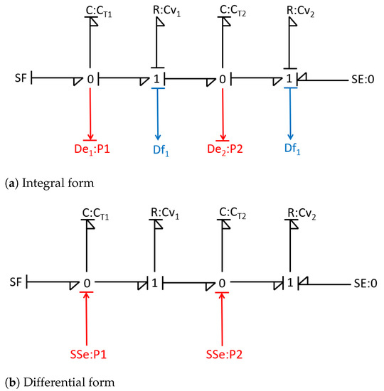
Figure 6.
Bond graph models of two-tank system.
That there are two types of detectors attached to the system. Efforts associated with the fluid level in tank 1 and 2 are measured using detectors and , respectively. The volume flow rate of fluid through valve 1 and valve 2 are measured using virtual detectors and . It must be noted that all the detectors are not always used together. and are used for system in differential causality. Therefore, these sensors are used for evaluation of ARRs and evaluation of Energy Activity in the differential form. and are used for a system in integral causality; hence, these sensors are used for evaluation of Energy Activity in the integral form. Evaluation of dual-EA requires all the detectors as this form includes both the differential and integral components.
The LFT bond graph used for calculation of ARRs and the corresponding residual bounds is shown in Figure 7. The generated ARRs are as follows:
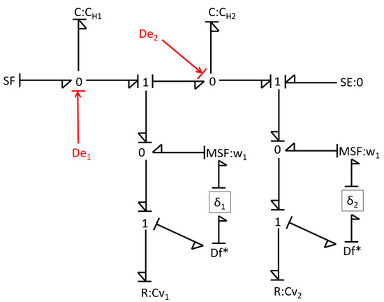
Figure 7.
LFT-bond graph model of 2-tank system.
The equations used for evaluation of Energy Activity in differential and integral forms are given in Table 4 and Table 5, respectively.
Table 4.
Effort and flow expressions for calculation of Energy Activity in differential form.
Table 5.
Effort and flow expressions for calculation of Energy Activity in the integral form.
The system is simulated to undergo a leakage in tank 1. A leak in the tank corresponds to a reduction in the nominal flow delivered by the pump. This reduction is expressed as a percentage of total volume delivered. The amount of leakage, i.e., the magnitude of fault, is considered very small. The fault magnitude variation over time under the different types of faults (abrupt, intermittent, and incipient) is shown in Figure 8. Figure 8a represents the abrupt fault in the system. To simulate this condition, the flow is decreased by 2% after 50 s from start, and this change is maintained throughout the remaining time. Figure 8b represents the intermittent fault in the system. The fault occurs randomly and vanishes after some time. The magnitude and duration for any fault step are not fixed. Figure 8c represents an incipient fault in the system. The fault starts at 75 s from the start of simulation and gradually increases to 2% at 1000 s.
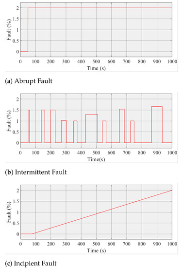
Figure 8.
Various types of faults measured as percentage change in ideal flow.
In addition, it is discussed in the previous section that Energy Activity for the most active component should be used for fault detection. For the parameters given in Table 3, the Energy Activity Index for an ideal system is measured for 1000 s. The variation of EAI of various components in the system is shown in Figure 9. From the figure, it is evident that tank 1 is the most active in the system. Therefore, Energy Activity evaluated at tank 1 is used for fault detection. Equations used for fault detection using differential, integral, and dual form are Equations (13)–(15). For the purpose of the current simulation, and in Equation (15) are both set to 1, thereby giving equal weights to both differential and integral components.
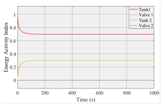
Figure 9.
Energy Activity Index for various components in ideal condition.
For the simulation using LFT-bond graph, it is noted that ARR1 (Equation (18)) is sensitive to the flow inlet to the system. As leakage is assumed as a reduction in flow input to the system, ARR1 is used for the simulation.
5. Simulation Results and Discussion
The system undergoes 3 types of faults, i.e., abrupt, intermittent, and incipient. For each fault, the system is simulated for 1000 s. The residual trends for fault detection (corresponding to Figure 8) using ARR method, Energy Activity in differential form, Energy Activity in the integral form, and Energy Activity in dual form are given by Figure 10, Figure 11, Figure 12, and Figure 13, respectively. For each of these figures, sub-figure a, b, and c show the generated residual for abrupt, intermittent, and incipient, respectively. The time taken for detection on various faults using the aforementioned methods is tabulated in Table 6.
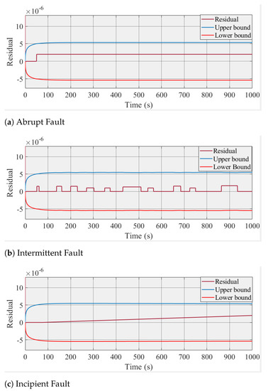
Figure 10.
Residuals generated for different types of faults using ARRs from LFT-bond graph.
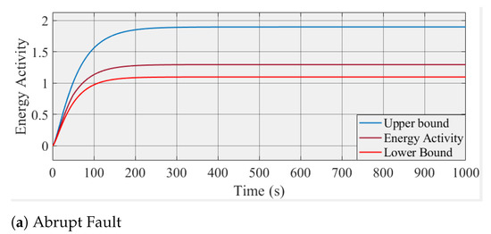
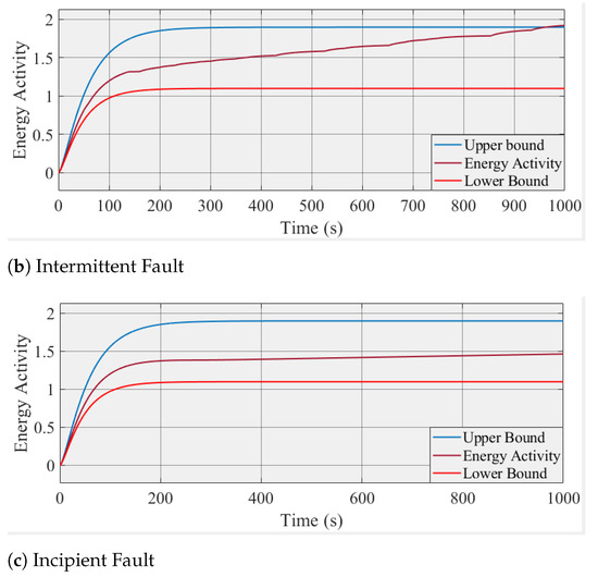
Figure 11.
Detection of different types of faults using Energy Activity in differential form.
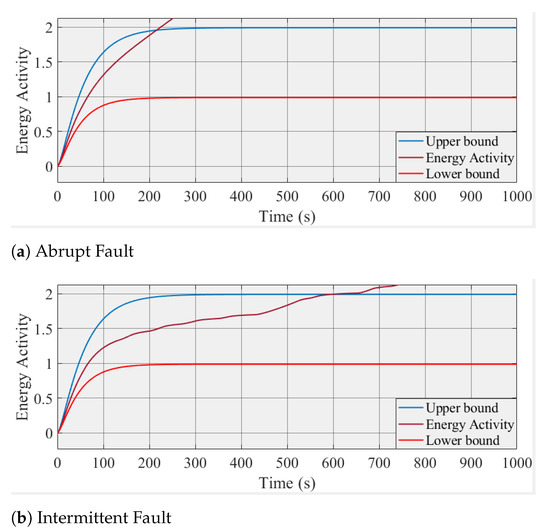
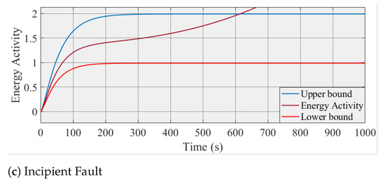
Figure 12.
Detection of different types of faults using Energy Activity in the integral form.
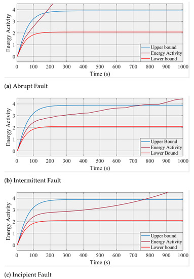
Figure 13.
Detection of different types of faults using Energy Activity in both integral and differential form.
Table 6.
Fault detection time.
From Table 6, it is observed that the residuals generated using ARR are unable to generate an alarm during the first 1000 s of simulation. From Figure 10, it can be observed that the residuals do conform to the fault signal for all the three types of faults. However, an alarm is not generated because the magnitude of the residuals are not high enough to overcome the bounds due to uncertainty. Figure 10c shows a continuous drift in the generated residual; so, the method will be able to detect the fault, but the fault magnitude will increase by that time, which is not desirable.
From Table 6, it is observed that the differential form of Energy Activity is able to detect intermittent faults during the stipulated time. However, the other faults are not detected in time. This is attributed to the fact that the change in EA depends on the rate of change of detected values. Therefore, as long as the system is not in a steady state, the calculated EA changes, and this calculated EA stabilizes when equilibrium is reached under faulty conditions. For intermittent faults (Figure 11b), due to numerous changes brought about by reoccurring faults, the total change in EA is big enough for detecting the fault. When a system is under an abrupt fault (Figure 11a), change in sensor values, i.e., energy distribution, occurs only once. Therefore, if the change brought about during the fault is not big enough, the fault is not detected. Figure 11c shows the EA under incipient fault. A drift in calculated EA is observed but is very small owing to the small rate of parameter degradation.
From Table 6, it is observed that the Energy Activity in the integral form is able to detect all three types of faults successfully, within the stipulated time. This is because, in its integral form, EA captures the total energy change in a component. Therefore, the generated residual in the faulty system continues to deviate, even when the system is stable. The amount of deviation caused is also proportional to the amount of error and the duration for which the system is under error. Therefore, an abrupt fault with a higher magnitude is captured in less time than the gradually increasing incipient fault, even though the duration of these errors is nearly the same.
From Table 6, it is observed that the dual-Energy Activity is also able to successfully detect all the three types of faults within the stipulated time. However, as compared to EA in the integral form, the dual form is faster in detecting the abrupt fault but slower in detecting intermittent and incipient faults. A possible reason can be that, for incipient and intermittent faults, the differential increase in residuals due to summation of differential and integral components is slower than the increase in the detection range. As the dual form is a mathematical summation of the differential and integral form, both its limits and residuals are a direct summation. The envelope of limits of dual form is twice that of the integral and differential form. On the other hand, a fast change due to high magnitude jump and retention of the fault causes a faster change in the differential component for the abrupt fault. This fast change, added to the integral component, propels the net residual beyond the allowed limits, to quickly generate the alarm.
The comparison of the discussed methods can be understood using Table 7.
Table 7.
Comparison of various fault detection methods.
6. Implementation on a Two-Tank System
The proposed fault detection method is implemented on a two-tank system (Figure 14) for checking the accuracy in working conditions. From the various simulations performed, the integral form of EA is used for the final application. As the real system measurements are never noise-free, the calculation of Energy Activity must be made robust to measurement noise.
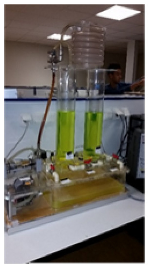
Figure 14.
Two-tank system.
Fault Detection is performed by continuous evaluation of EA in time domain. Therefore, noise is adjusted in the calculation of EA.
where S power variable input to the component. S is always a measured quantity; therefore, for noise accommodation, S is replaced with , where is the uncertain component of the measurement.
Assuming an LTI behavior of the system for the duration of calculation of Energy Activity, Equation (21) can be expanded as shown in Equation (22):
For measurements with high signal to noise ratio, can be neglected from Equation (22). So, EA can be calculated using Equation (23).
as
Therefore, inequality relation relation can be applied to Equation (23) in the form shown be Equation (25).
The above equation can be combined with Equation (26) to obtain the limits to EA, incorporating both model and measurement uncertainties. The lower and upper limit of EA ( and , respectively) can then be calculated as:
and are the maximum and minimum allowed Energy Activity after accommodating the uncertainty in the system component values.
is the error in the component input due to noise. As noise can be either positive or negative, the r.m.s. value of error is noise is used for calculation of and .
The method is checked for two types of faults, i.e., an actuator fault and a system fault. The actuator fault is introduced by changing the flow input to the system and system fault is introduced by opening the leakage valve in the tank 1. For both of the above, small incipient faults are introduced. The system is considered immune from intermittent faults from the environment. The r.m.s. error for measurement is known ( m3/s).
Measured flow through valve 1 (Figure 15a) and Energy Activity calculated at tank 1 (Figure 15b) for a two-tank system undergoing leakage in tank 1 is shown in Figure 15. A leakage in tank represents a system fault. Similarly, a system with an actuator fault, i.e., faulty pump, is shown in Figure 16. From the above figures, it is evident that minute incipient faults are detected using EA in the integral form under both system and measurement uncertainty.
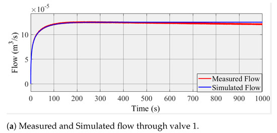
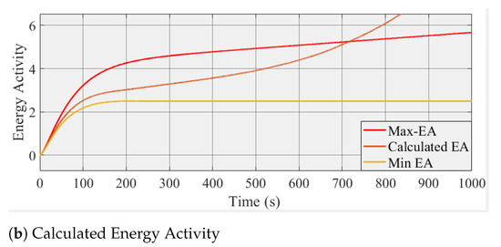
Figure 15.
Flow through valve 1 and Energy Activity for two-tank system undergoing leakage in tank 1.
Figure 16.
Flow through valve 1 and Energy Activity for two-tank system with faulty pump.
7. Conclusions and Future Works
In this paper, the problem of missed alarms in model-based fault detection techniques, due to high uncertainty in certain components and measurements, is addressed. To overcome this problem, an energy-based metric is proposed which can also utilize the fault history and is isolated from the influence of uncertain components. Energy Activity, which has all the desired properties is proposed as metric for fault detection. Three forms of energy activity, i.e., differential, integral, and dual, are developed. The three forms are compared with each other and with fault detection residuals generated from Analytical Redundancy Relations. The above methods are simulated on a two-tank system, and the results are compared. The comparison is based on the ability of a method to detect minute faults and time taken by all the aforementioned methods for detecting three types of faults, i.e., abrupt fault, incipient fault, and intermittent fault, representing discrete fault, degradation, and fault due to external influence, respectively. The fault magnitude is considered small, and the performance of the methods depend on how quickly can the fault be identified. All the forms of Energy Activity perform better than residuals from ARR. However, EA in the integral form performs best among the various forms of EA for detecting degradation and faults due to external influence. EA in dual form performs best for detecting discrete faults. Therefore, as a general notion, it is suggested that EA in the integral form should be used for fault detection using. The proposed form is tested on a real two-tank system, and noise accommodation method for EA in the integral form is also presented. It should be noted that, in the proposed integral form, robust fault detection can be achieved without the need for any signal filtering. The proposed method is checked for two types of fault, i.e., actuator fault and a system fault, due to a fault in the inlet pump and a leakage in tank, respectively. The proposed method is able to detect minute incipient faults correctly. A limitation for the use of EA can be high computation and memory requirements. High computation power is required because a virtual system is simulated in parallel to the real system. High memory requirements can be due to the very high numeric values of the EA which can arise in a highly dynamic system. Another limitation can be the requirements of the system details, such as uncertainty in all the system components and measurements, before the method can be used. In the future, the dual-EA form can be improved by developing methods for calibrating the gains for differential and integral components.
Author Contributions
Conceptualization, M.S.; methodology, M.S.; validation, M.S.; formal analysis, M.S.; writing—original draft preparation, M.S.; writing—review and editing, M.S. and A.-L.G.; supervision, A.-L.G. and B.O.-B. All authors have read and agreed to the published version of the manuscript.
Funding
This research received no external funding.
Institutional Review Board Statement
Not applicable.
Informed Consent Statement
Not applicable.
Data Availability Statement
Not applicable.
Conflicts of Interest
The authors declare no conflict of interest.
References
- Jouin, M.; Bressel, M.; Morando, S.; Gouriveau, R.; Hissel, D.; Péra, M.C.; Zerhouni, N.; Jemei, S.; Hilairet, M.; Ould-Bouamama, B. Estimating the end-of-life of PEM fuel cells: Guidelines and metrics. Appl. Energy 2016, 177, 87–97. [Google Scholar] [CrossRef]
- Yoon, S.; MacGregor, J.F. Fault diagnosis with multivariate statistical models part I: Using steady state fault signatures. J. Process. Control. 2001, 11, 387–400. [Google Scholar] [CrossRef]
- Artés, M.; Del Castillo, L.; Pérez, J. Failure prevention and diagnosis in machine elements using cluster. In Proceedings of the Tenth International Congress on Sound and Vibration, Stockholm, Sweden, 7–10 July 2003; pp. 1197–1203. [Google Scholar]
- Qin, S.J. Survey on data-driven industrial process monitoring and diagnosis. Annu. Rev. Control. 2012, 36, 220–234. [Google Scholar] [CrossRef]
- Zhu, F.; Tang, Y.; Wang, Z. Interval-Observer-based Fault Detection and Isolation Design for T-S Fuzzy System Based on Zonotope Analysis. IEEE Trans. Fuzzy Syst. 2021. [Google Scholar] [CrossRef]
- Abid, A.; Khan, M.T.; Iqbal, J. A review on fault detection and diagnosis techniques: Basics and beyond. Artif. Intell. Rev. 2021, 54, 3639–3664. [Google Scholar] [CrossRef]
- Liu, R.; Yang, B.; Zio, E.; Chen, X. Artificial intelligence for fault diagnosis of rotating machinery: A review. Mech. Syst. Signal Process. 2018, 108, 33–47. [Google Scholar] [CrossRef]
- Yuwono, M.; Qin, Y.; Zhou, J.; Guo, Y.; Celler, B.G.; Su, S.W. Automatic bearing fault diagnosis using particle swarm clustering and Hidden Markov Model. Eng. Appl. Artif. Intell. 2016, 47, 88–100. [Google Scholar] [CrossRef]
- Djeziri, M.A.; Benmoussa, S.; Zio, E. Review on health indices extraction and trend modeling for remaining useful life estimation. In Artificial Intelligence Techniques for a Scalable Energy Transition; Springer: Cham, Switzerland, 2020; pp. 183–223. [Google Scholar]
- Mojallal, A.; Lotfifard, S. Multi-physics graphical model-based fault detection and isolation in wind turbines. IEEE Trans. Smart Grid 2017, 9, 5599–5612. [Google Scholar] [CrossRef]
- Ekanayake, T.; Dewasurendra, D.; Abeyratne, S.; Ma, L.; Yarlagadda, P. Model-based fault diagnosis and prognosis of dynamic systems: A review. Procedia Manuf. 2019, 30, 435–442. [Google Scholar] [CrossRef]
- Venkatasubramanian, V.; Rengaswamy, R.; Kavuri, S.N. A review of process fault detection and diagnosis: Part II: Qualitative models and search strategies. Comput. Chem. Eng. 2003, 27, 313–326. [Google Scholar] [CrossRef]
- Djeziri, M.A.; Merzouki, R.; Ould-Bouamama, B.; Dauphin-Tanguy, G. Robust fault diagnosis by using bond graph approach. IEEE/ASME Trans. Mechatronics 2007, 12, 599–611. [Google Scholar] [CrossRef]
- Jha, M.S.; Dauphin-Tanguy, G.; Ould-Bouamama, B. Robust FDI based on LFT BG and relative activity at junction. In Proceedings of the 2014 European Control Conference (ECC), Strasbourg, France, 24–27 June 2014; pp. 938–943. [Google Scholar]
- Milanese, M.; Norton, J.; Piet-Lahanier, H.; Walter, É. (Eds.) Bounding Approaches to System Identification; Springer Science & Business Media: Boston, MA, USA, 2013. [Google Scholar]
- Herrero, P.; Calm, R.; Vehí, J.; Armengol, J.; Georgiou, P.; Oliver, N.; Tomazou, C. Robust fault detection system for insulin pump therapy using continuous glucose monitoring. J. Diabetes Sci. Technol. 2012, 6, 1131–1141. [Google Scholar] [CrossRef]
- Song, Y.; Zhong, M.; Xue, T.; Ding, S.X.; Li, W. Parity space-based fault isolation using minimum error minimax probability machine. Control. Eng. Pract. 2020, 95, 104242. [Google Scholar] [CrossRef]
- Shang, C.; Ding, S.X.; Ye, H. Distributionally robust fault detection design and assessment for dynamical systems. Automatica 2021, 125, 109434. [Google Scholar] [CrossRef]
- Stojanovic, V.; Prsic, D. Robust identification for fault detection in the presence of non-Gaussian noises: Application to hydraulic servo drives. Nonlinear Dyn. 2020, 100, 2299–2313. [Google Scholar] [CrossRef]
- Shafai, B.; Moradm, A. Design of an integrated observer structure for robust fault detection. In Proceedings of the 2020 IEEE Conference on Control Technology and Applications (CCTA), Montreal, QC, Canada, 24–26 August 2020; pp. 248–253. [Google Scholar]
- Dong, X.; He, S.; Stojanovic, V. Robust fault detection filter design for a class of discrete-time conic-type non-linear Markov jump systems with jump fault signals. IET Control. Theory Appl. 2020, 14, 1912–1919. [Google Scholar] [CrossRef]
- Yin, Y.; Shi, J.; Liu, F.; Liu, Y. Robust fault detection of singular Markov jump systems with partially unknown information. Inf. Sci. 2020, 537, 368–379. [Google Scholar] [CrossRef]
- Wei, Y.; Wu, D.; Terpenny, J. Robust incipient fault detection of complex systems using data fusion. IEEE Trans. Instrum. Meas. 2020, 69, 9526–9534. [Google Scholar] [CrossRef]
- Safizadeh, M.S.; Golmohammadi, A. Ball bearing fault detection via multi-sensor data fusion with accelerometer and microphone. Insight-Non-Destr. Test. Cond. Monit. 2021, 63, 168–175. [Google Scholar]
- Li, S.; Wang, H.; Song, L.; Wang, P.; Cui, L.; Lin, T. An adaptive data fusion strategy for fault diagnosis based on the convolutional neural network. Measurement 2020, 165, 108122. [Google Scholar] [CrossRef]
- Azamfar, M.; Singh, J.; Bravo-Imaz, I.; Lee, J. Multisensor data fusion for gearbox fault diagnosis using 2-D convolutional neural network and motor current signature analysis. Mech. Syst. Signal Process. 2020, 144, 106861. [Google Scholar] [CrossRef]
- Mukherjee, A.; Karmakar, R.; Samantaray, A.K. Bond Graph in Modeling, Simulation and Fault Identification; IK International: New Delhi, India, 2006; pp. 342–346. [Google Scholar]
- Karnopp, D.C.; Margolis, D.L.; Rosenberg, R.C. System Dynamics: Modeling, Simulation, and Control of Mechatronic Systems; John Wiley & Sons: Hoboken, NJ, USA, 2012. [Google Scholar]
- Ould-Bouamama, B.; Samantaray, A.K.; Staroswiecki, M.; Dauphin-Tanguy, G. Derivation of constraint relations from bond graph models for fault detection and isolation. Simul. Ser. 2003, 35, 104–109. [Google Scholar]
- Jha, M.S. Diagnostics and Prognostics of Uncertain Dynamical Systems in a Bond Graph Framework. Doctoral Dissertation, Ecole Centrale de Lille, Villeneuve-d’Ascq, France, 2015. [Google Scholar]
- Louca, L.S.; Stein, J.L.; Hulbert, G.M. A physical-based model reduction metric with an application to vehicle dynamics. IFAC Proc. Vol. 1998, 31, 585–590. [Google Scholar] [CrossRef]
- Louca, L.S. A frequency-based interpretation of energy-based model reduction of linear systems. J. Dyn. Syst. Meas. Control. 2016, 138. [Google Scholar] [CrossRef]
- Singh, M.; Ould-Bouamama, B.; Gehin, A.L.; Kumar, P. Bond graph model for prognosis and health management of mechatronic systems based on energy activity. In Proceedings of the 2018 7th International Conference on Systems and Control (ICSC), Valencia, Spain, 24–26 October 2018; pp. 430–434. [Google Scholar]
- Singh, M.; Gehin, A.L.; Bouamama, B.O. Prognosis and Health Management using Energy Activity. IFAC-PapersOnLine 2020, 53, 10310–10317. [Google Scholar] [CrossRef]
- Adrot, O.; Maquin, D.; Ragot, J. Fault detection with model parameter structured uncertainties. In Proceedings of the 1999 European Control Conference (ECC), Karlsruhe, Germany, 31 August–3 September 1999; pp. 475–480. [Google Scholar]
- Sainz, M.Á.; Armengol, J.; Vehı, J. Fault detection and isolation of the three-tank system using the modal interval analysis. J. Process. Control. 2002, 12, 325–338. [Google Scholar] [CrossRef]
- Hickey, T.; Ju, Q.; Van Emden, M.H. Interval arithmetic: From principles to implementation. J. ACM (JACM) 2001, 48, 1038–1068. [Google Scholar] [CrossRef]
- Caprani, O.; Madsen, K.; Rall, L.B. Integration of interval functions. SIAM J. Math. Anal. 1981, 12, 321–341. [Google Scholar] [CrossRef][Green Version]
- Jha, M.S.; Dauphin-Tanguy, G.; Ould-Bouamama, B. Robust fault detection with interval valued uncertainties in bond graph framework. Control. Eng. Pract. 2018, 71, 61–78. [Google Scholar] [CrossRef]


Publisher’s Note: MDPI stays neutral with regard to jurisdictional claims in published maps and institutional affiliations. |
© 2021 by the authors. Licensee MDPI, Basel, Switzerland. This article is an open access article distributed under the terms and conditions of the Creative Commons Attribution (CC BY) license (https://creativecommons.org/licenses/by/4.0/).