Abstract
Effective gas dispersion and liquid mixing are significant parameters in the design of an inert-particle spouted-bed reactor (IPSBR) system. Solid particles can be used to ensure good mixing and an efficient rate of mass and heat transfer between the gas and liquid. In this study, computational fluid dynamics (CFD) coupled with the discrete phase model (DPM) were developed to investigate the effect of the feed gas velocity (0.5–1.5 m/s), orifice diameter (0.001–0.005 m), gas head (0.15–0.35 m), particle diameter (0.009–0.0225 m), and mixing-particle-to-reactor-volume fraction (2.0–10.0 vol.%) on the solid mass concentration, average solid velocity, and average solid volume fraction in the upper, middle, and conical regions of the reactor. Statistical analysis was performed using a second-order response surface methodology (RSM) with central composite design (CCD) to obtain the optimal operating conditions. Selected parameters were optimized to maximize the responses in the middle and upper regions, and minimize them in the conical region. Such conditions produced a high interfacial area and fewer dead zones owing to good particle dispersion. The optimal process variables were feed gas velocity of 1.5 m/s, orifice diameter of 0.001 m, gas head of 0.2025 m, a particle diameter of 0.01 m, and a particle load of 0.02 kg. The minimum average air velocity and maximum air volume fraction were observed under the same operating conditions. This confirmed the novelty of the reactor, which could work at a high feed gas velocity while maintaining a high residence time and gas volume fraction.
1. Introduction
Spouted beds have several advantages and potential applications compared to moving beds. They can handle granular particles with a wide size distribution range, provide an efficient mixing between the solid and gas phases and significant rates of heat and mass transfer [1,2,3,4,5,6,7,8]. Inert particles spouted bed reactor (IPSBR) is a spouted bed in which a gas jet is injected at the bottom of a conical vessel containing liquid and inert particles [9]. El-Naas et al. [10,11] developed and investigated a novel IPSBR to deal with both CO2 capture and reject brine management. Their results indicated that the CO2 capture efficiency reached up to 97.7% at a gas-to-liquid volume ratio of 123. They also concluded that the interfacial area between the gas and liquid was enhanced using inert gas particles. This was due to the circular motion of the particles inside the reactor, which enhanced the CO2 capture efficiency and ion removal [6]. The hydrodynamics of the same IPSBR were studied by Mohammad et al. [12,13,14]. They used computational fluid dynamics (CFD) with ANSYS Fluent and Eulerian models to examine the influence of mixing particles on the velocity distribution, gas spreading, and eddy viscosity stresses inside the reactor [13]. In addition, they studied the effects of operating conditions (i.e., feed-gas velocity, orifice diameter, gas head, mixing-particle diameter, and mixing-particle loading) on the average air velocity and air volume fraction in three contact system sectional areas (i.e., the conical, middle, and upper regions) [4]. The results indicated that the conical part of the reactor, along with the mixing particles, enhanced the circulation and gas dispersion in the liquid. It also increased the residence time and gas hold-up [13]. According to the researchers, the optimum response were found when the gas velocity was 1.5 m/s, the orifice diameter was 0.001 m, the gas head was 0.164 m, the mixing particle diameter was 0.0220 m, and the mixing-particle loading was 0.02 kg [13]. The results were validated using a bench-scale IPSBR. A good agreement was found between the experiments and the model calculations [12,13,14].
The optimization of various operating parameters for the reactor mentioned above is still under investigation. It is essential for the reactor’s design, pilot plant scale-up, and industrial operation [13]. The focus of the current work is to understand the interactions between the most effective factors, which will result in good particle distribution throughout the reactor. Accordingly, more responses will be introduced to the response surface design to confirm additional precise optimum conditions to be used in real CO2 capturing reaction using the IPSBR system.
Kim et al. [4] established a CFD model for two reactors that had a diameter of 2.2 m and a height of 6.0 m. The CFD results for the gas holdup, interfacial area, and mass transfer were tested by the experimental results and empirical correlations published in the literature. However, the CFD results for CO2 capture efficiency were compared with pilot plant data. They determined that the error for these parameters was in the range of 1–8%. Su et al. [15] investigated the hydrodynamics of a slurry bed by CFD-PBM using a modified drag force model. The results displayed that the modified model could be used to evaluate the flow hydrodynamics in the existence of particles. Their results demonstrated that bubble coalescence had been enhanced; thus, large-diameter (more velocity) bubbles were formed by increasing the particle load. This parameter should have been controlled, as it reduced the gas holdup in the reactor. They also stated that the uniformity of the particle flow was decreased by increasing the superficial gas velocity. A CFD simulation, namely Fluent, was developed by Yancheshme et al. [16] to model a 2D cylindrical bubble column with a diameter of 0.49 m, height of 3.6 m, and superficial gas velocity of 0.14 m/s under unsteady-state conditions. The dispersed phase was the air, whereas the continuous phase was water, which operated in the churn–turbulent flow regime. It was concluded that the bubble size distribution at the inlet of the column did not affect the distribution inside the column. Lakhdissi et al. [17] investigated the impact of particle diameter and concentration on gas holdup for a slurry bubble column. The process consisted of three phases (air, water, and glass beads). Their results indicated that the gas holdup was reduced by increasing the particle diameter and solids concentration. In addition, a novel correction factor was implemented to consider the additional impact of particles on bubble flow with regard to the collision aspect. In a study conducted by Sasaki et al. [18], the effect of several superficial gas velocities, mean particle volumetric concentrations, and initial slurry heights on gas holdup were examined. They concluded that for 100-μm silica particles, the gas holdup decreased as the concentration was increased up to 0.40. However, the holdup was independent at higher concentrations. They also mentioned that, in general, increasing the solids concentration reduces the gas holdup and therefore increases the bubble diameter [17]. Rabha et al. [19] examined the effect of particle size (50–150 µm) and solids concentration Cs of (0–0.20) on the hydrodynamics of a slurry bubble column by utilizing ultrafast electron beam X-ray tomography. The experiment was conducted at a superficial gas velocity of between 0.02 and 0.05 m/s. It was observed that when the particle size and solids concentrations were less than 100 µm and 3%, respectively, the average gas holdup was independent of them. However, at larger diameters and solids concentrations, they detected that the average gas holdup was decreased remarkably by increasing the size and concentration of the particles. Many studies [20,21] are in agreement with Rabha et al. [19], and it has been reported that by increasing the particle size, the gas holdup decreased. The effect of particle size (60–150 µm) and particle volumetric concentration (0% to 50%) on gas holdup was investigated by Ojima et al. [22]. Their results indicated that the bubble coalescence increased by decreasing the particle size and increasing the concentration of solids; thus, the gas holdup was decreased.
Gholamzadehdevin et al. [23] studied the hydrodynamic performance of an activated-sludge bubble column. They combined CFD (Eulerian–Eulerian) and the design of the experiment (full-factorial design) to obtain the influence of superficial gas velocity, tracer injection position, and sparger type on the mixing time. Their findings indicated a strong connection between the superficial gas velocity and the location of the tracer injection on the mixing time. Moreover, the hydrodynamic performance was improved by a modified star-shaped gas sparger. Central composite design was used to optimize the operating conditions of the bubble column (piperazine–H2O–CO2) [24]. The results indicated that the maximum value (97.7%) of CO2 capture could be achieved with a piperazine concentration of 0.162 M, solution flow rate of 0.502 L/h, CO2 flow rate of 2.199 L/min, and stirrer speed of 68.89 rpm. They mentioned that the p-values of the dependent parameters were under 0.05, which reflected their significance and importance. Song et al. [25] developed a new cryogenic process based on free-piston Stirling coolers to enhance the CO2 removal efficiency. They used response surface methodology (RSM) to optimize the operating conditions. They concluded that the process could capture up to 95.20% of the CO2 under the optimal conditions of 2.16 L/min flowrate, temperature of −18 °C, and operation time of 3.9 h.
In light of the literature mentioned above, much helpful information has been reported on the impact of operating conditions on the hydrodynamics and bubble behavior of various bubble column reactors. The literature also reveals the importance of optimizing the operating parameters of the reactor, as they have an observable potential for enhancing the design and overall performance of the process. However, there is still a lack of information on optimizing the most effective hydrodynamic parameters (feed gas velocity, orifice diameter, gas head, diameter of mixing particles and mixing particle load) of an IPSBR. Optimization of various operating parameters for the IPSBR is still under investigation, and it is essential for the design, pilot plant scale-up, and industrial operation of the reactor. The current work focuses on understanding the interactions between the most effective factors resulting in good particle distribution throughout the reactor. Accordingly, more responses are introduced to the response surface design to ensure more accurate optimum conditions for real CO2 capture reactions using the IPSBR system. Therefore, the main objective of the present study is to combine the CFD model with RSM analysis to study the impact of these variables on the mass concentration, average velocity, and average volume fraction of mixing particles throughout the reactor. The combination of the CFD model and RSM analysis enables the prediction of the best conditions at which the solid particles are dispersed perfectly to obtain high gas hold-up, greater interfacial area, and longer residence time.
2. CFD Simulation
2.1. Simulation Configuration
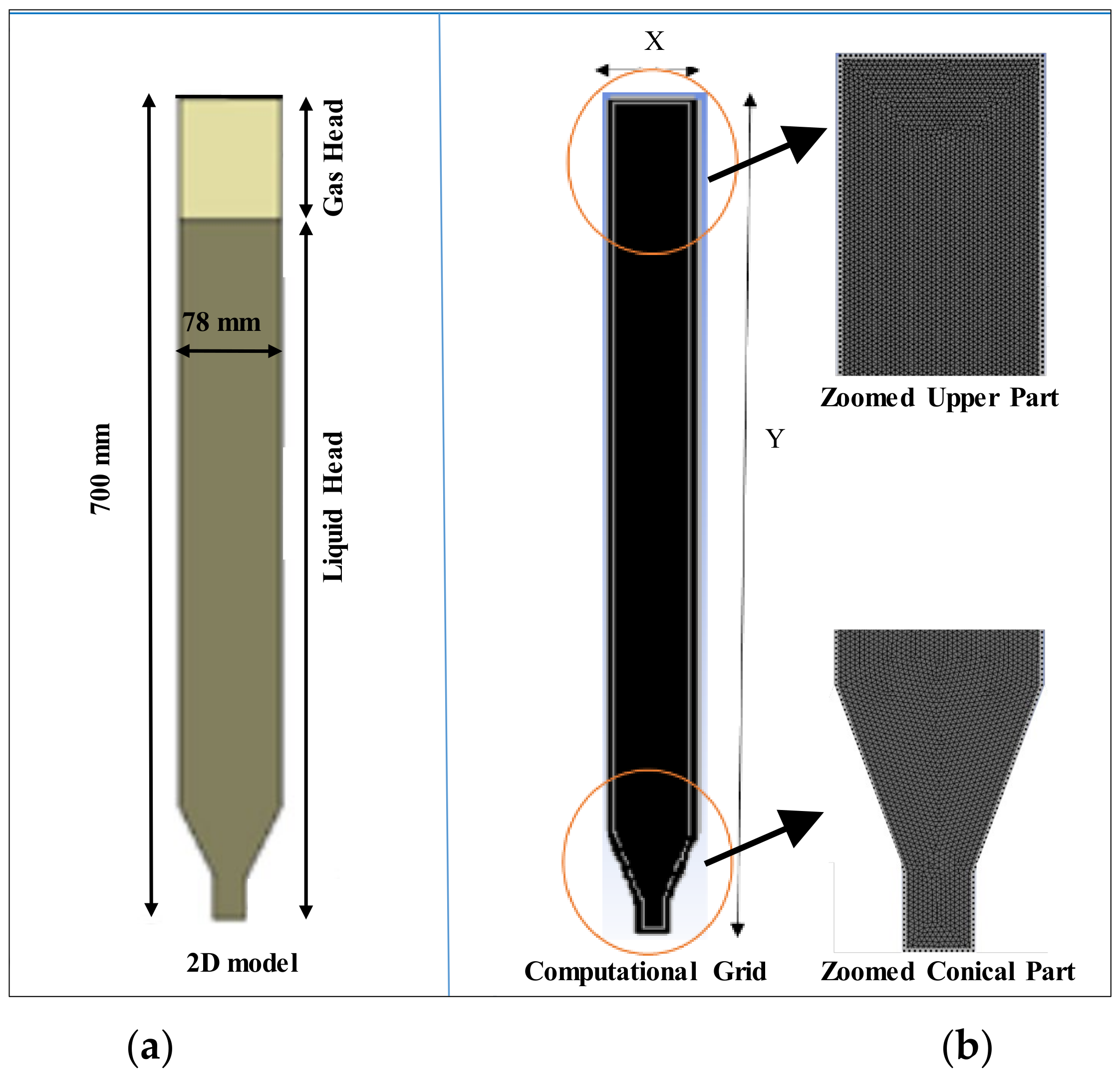
ANSYS Fluent 18.0 (CFD) combined with Eulerian multiphase was used to model the axisymmetric of a 2D IPSBR, which was working in a semi-batch mode. The simulated reactor configuration was sourced from a previous study, as shown in Figure 1 [12]. The simulation was conducted with three phases (air, water, and solid). The solid phase consisted of polymethyl methacrylate particles (average density of 1020 kg/m3 and average particle size of 0.013 m). First, the simulated IPSBR reactor was filled with a specific amount of water. An air space (gas head) was retained at the top of the reactor because the water level would rise once the gas started to flow [12,13]. Mohammad et al. performed a mesh independence study [12] and concluded that a grid size of 0.0020 (cell count = 3287) would be sufficient and could be applied in this study. An intensive mesh study was conducted by a previous research study [12,13]. The simulation runs were all converged. Seven meshes with mesh sizes ranging from 0.0022 to 0.0016 were tested (22,845, 28,568, 32,871, 36,112, 39,068, 41,386, and 42,372). The air velocity convergence was achieved at a mesh size of 0.0016, which was only about 1% different from the previous mesh size. The oscillation-shaped solution was found to be mesh-independent, with no significant differences between the last four mesh sizes. As a result, in the 2D column runs, the grid size of 0.0020 was used, which results in a 2.6% difference from the finest mesh.

Figure 1.
(a) IPSBR system with 2D vertical cross section and simulated model with major dimensions and gas/liquid heads, and (b) the computational grid and mesh structure for the CFD model [12,13].
2.2. CFD Model
The Eulerian multiphase model in the commercial CFD software package Fluent 18.0 was used to model and investigate the hydrodynamic flow behavior of the IPSBR system under transient and gravitational acceleration operational conditions. All runs were carried out under isothermal and unsteady-state behavior. In addition, gas was considered to have constant properties, which was considered as the secondary phase and the liquid as the main phase. The top of the reactor was open to the atmosphere. Bubbles of equal diameter (0.001–0.005 m) were created at the bottom of the reactor through a spherical orifice with a specific diameter. A very small step size of 0.00001 s was employed with 20 iterations for each time step. The convergence criterion was identified to be 10−3 for the relative error between two sequential iterations. To solve the numerical model, a finite volume method was employed. Turbulence was simulated using the standard k-ɛ mixture model using wall functions (low-Re k-ɛ near the wall). The discrete phase model (DPM) was implemented to consider the impact of mixing particles. CFD describes the fluid phase by solving the Navier–Stokes equations. The particle velocities and forces are calculated in DEM by solving Newton’s equations of motion. The time it takes to record converged results is 20 s or longer. The transient state’s time-averaged profile was previously calculated at 25 and 30 s time intervals (averaged data over 5 s of flow was chosen) [12]. In this work, the time-averaged profile for the transient state has been selected to be over 60 to 65 s time intervals to insure more stability of the quasi steady state condition. The standard error deviation was in the range of (0.00429–0.00961) [13]. The equations are listed in Table 1. More information and details can be found in the preceding research work [12,13].

Table 1.
Governing equations and correlations.
3. Response Surface Methodology (RSM) Design
Central composite design (CCD) is a frequently used form of RSM that affords the opportunity to study interactions between the independent process parameters and dependent process responses [31,32,33,34,35,36,37,38]. In this study, a full-factorial CCD design was carried out using Minitab 19.0 to investigate the influence of input parameters (i.e., feed gas flowrate, orifice diameter, gas head, mixing particle diameter, and mixing particles load) on the responses (i.e., mass concentration, average velocity, and average volume fraction of the mixing particles) throughout the reactor. Table 2 listed the levels of the independent parameters and the consistent variation levels used to optimize the process conditions. Thirty-two runs with five levels of each parameter were designated. The conditions of each run were entered into the ANSYS software, and all of the data attained were analyzed using the Minitab software (RSM).
Table 2.
Levels of independent parameters of CCD runs.
4. Results and Discussion
4.1. Impact of Independent Parameters on Average Solid Velocity Distribution
- (a)
- Effect of feed gas velocity on average solid velocity distribution
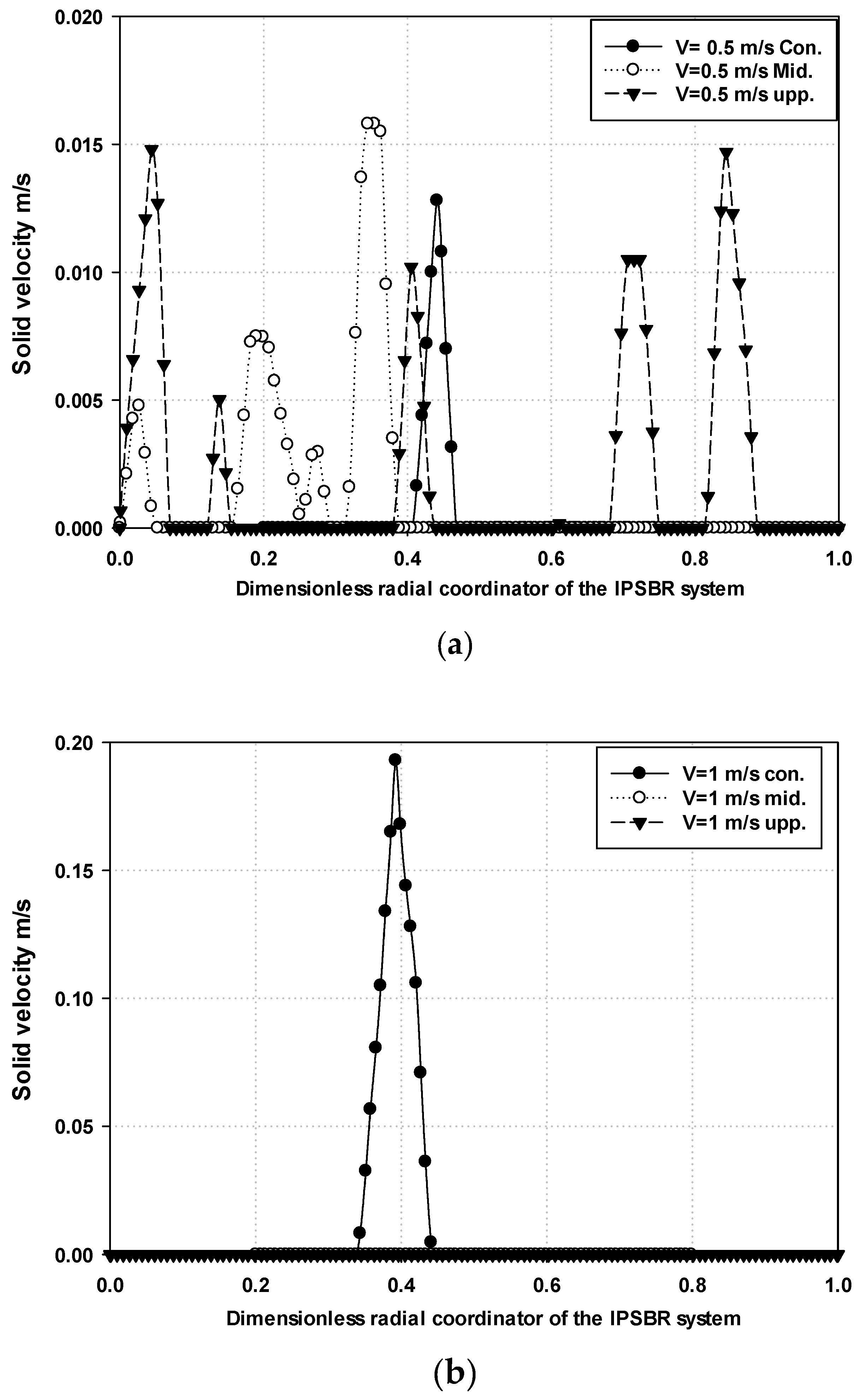
Figure 2a–c illustrates the effect of the feed gas velocity (0.5, 1, and 1.5 m/s) on the average solid velocity distribution in the conical, upper, and middle regions versus the dimensionless radial coordinate (R), which represents the dimensionless diameter of the IPSBR system, where R = 0.0 and R = 1.0 are the IPSBR system walls in the 2D model. The results were observed at a constant orifice diameter of 0.003 m, gas head of 0.25 m, mixing particle diameter of 0.0135 m, and total mass of mixing particles of 0.06 kg. It is clear from the figures that the effect of a feed gas velocity of 1.5 m/s had a significant effect on the average solid velocity distribution in the middle region and reached a maximum value of 0.014 m/s. At a feed gas velocity of 1 m/s, the influence was observed more in the conical region compared with the middle and upper regions. By contrast, at a minimum feed gas velocity of 0.5 m/s, the solids existed in almost all of the regions of the reactor. Due to the no-slip boundary condition, the solid velocity was almost zero at the wall for all values of feed gas velocity. It is worth noting that the solid particle velocity was detected in the three system zones at low gas velocity of 0.5 m/s, as shown in Figure 2a. However, when the particle velocity was increased to 1 m/s and 1.5 m/s, most of the detected velocities were zero; this could be explained by accelerating the solid particles in the studied surface zone and thus the disappearance/absence of these solid particles, as shown in Figure 2b,c.
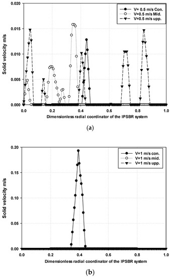
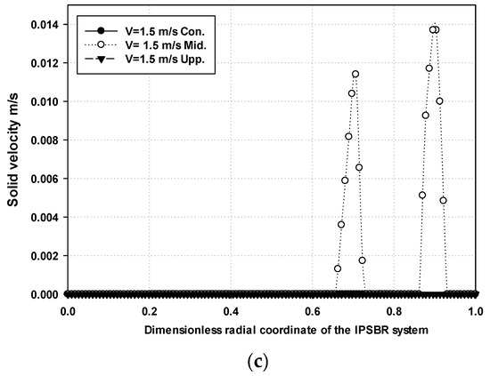
Figure 2.
Effect of feed gas velocity ((a) 0.5 m/s, (b) 1 m/s, and (c) 1.5 m/s) on the average solid velocity at a constant orifice diameter of 0.003 m, gas head of 0.25 m, mixing particle diameter of 0.0135 m, and total mass of mixing particle of 0.06 kg in the conical, middle, and upper regions.
- (b)
- Effect of Orifice Diameter on Average Solid Velocity
Figure S1a,b depicts the effect of two different orifice diameters (0.003 and 0.005 m) on the average solid velocity in the three regions. The results were extracted for a constant feed gas velocity of 1 m/s, gas head of 0.25 m, mixing particle diameter of 0.0135 m, and mixing particle load of 0.06 kg. It was found that increasing the orifice diameter from 0.003 to 0.005 m reduced particle velocity throughout the upper region and made it easier to detect, as shown in Figure S1b. The mixing particles, on the other hand, were not detected when a smaller orifice diameter was used, as shown in Figure S1a. It is clear from Figure S1b that the particle velocity was not detected in the conical and middle regions. Whereas, in the upper region it reached a peak value of almost 0.1 m/s. This is also connected to the gas velocity inside the reactor, which increased inside the reactor at higher orifice diameters, owing to the creation of larger bubble sizes. Because of that, the particles would not be well distributed in a uniform profile throughout the reactor at higher orifice diameters [36].
- (c)
- Effect of gas head on average solid velocity
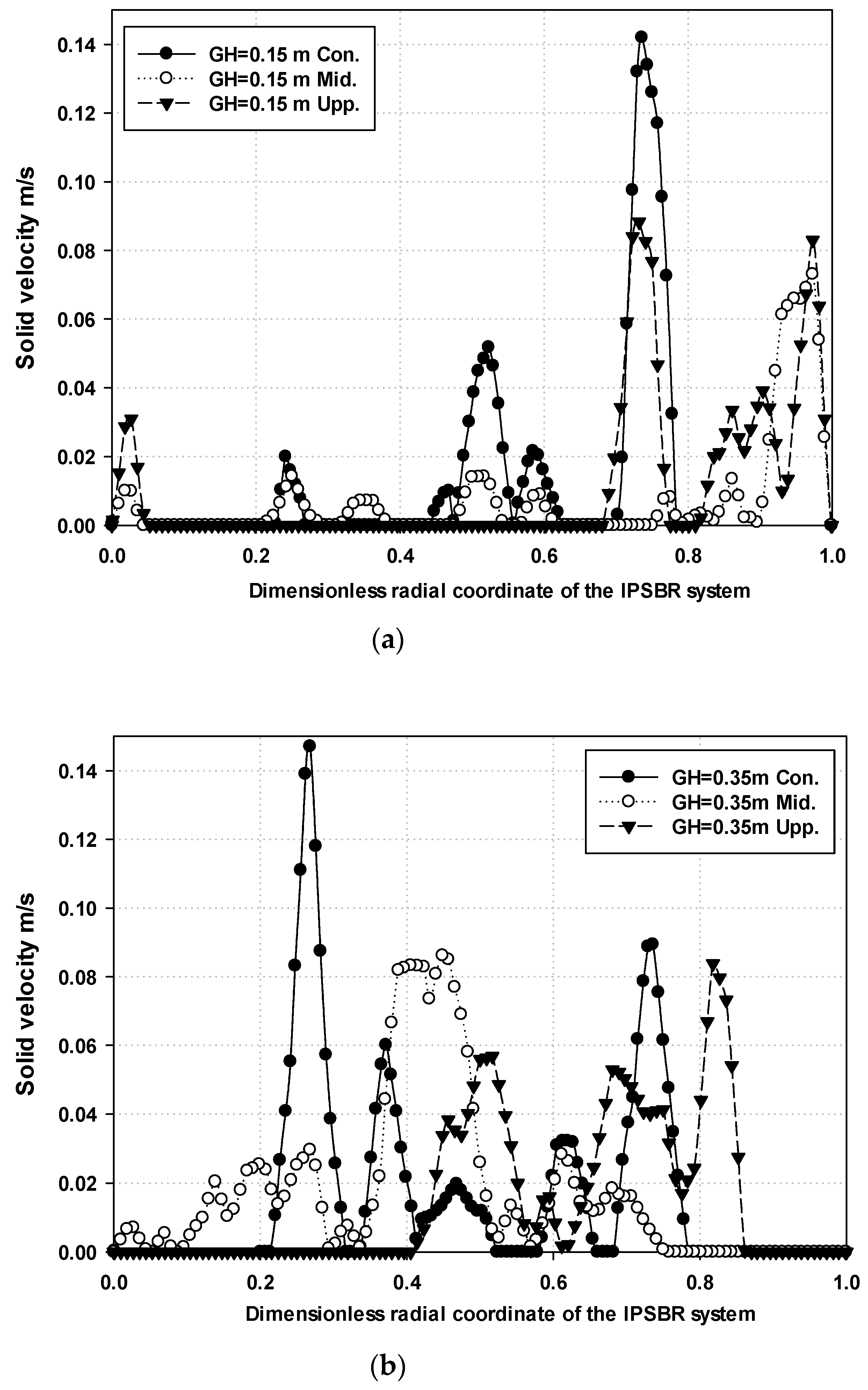
The effect of gas head on the average solid velocity distribution was studied at a constant feed gas velocity of 1 m/s, 0.003 m orifice diameter, mixing particle diameter of 0.0135 m, and total mass of mixing particle of 0.06 kg in all three regions. In the conical region, it was expected to see high dispersion and turbulence of the particle distribution because that is the injection zone for those particles. Furthermore, the cross-sectional area of the conical region was smaller than those of the middle and upper regions. Therefore, a clear behavior was not detected in conical region. It can be seen in Figure 3a,b that more gas head resulted in an increase in the particle velocity in the middle and upper regions. From the simulated data of a gas head value of 0.15 m, it was found that the mixing particles at R = 0.2 to 0.6 had an average velocity of around of 0.04 m/s. However, in the same section with a gas head value of 0.35 m, the average solid velocity approached a value of around 0.06 m/s. A lower gas head meant a higher liquid level. As the liquid level increased this exerted more pressure on the mixing particles; therefore, a lower particle velocity was observed.
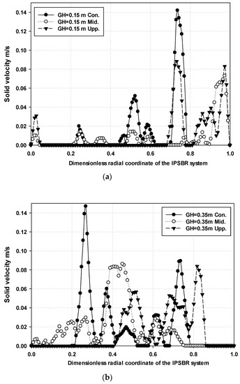
Figure 3.
Effect of gas head ((a) 0.15 m and (b) 0.35 m) on the average solid velocity at a constant feed gas velocity of 1 m/s, orifice diameter of 0.003 m, mixing particle diameter of 0.0135 m, and total mass of mixing particle of 0.06 kg in the conical, middle, and upper regions.
- (d)
- Effect of mixing particle diameter on average solid velocity
The influence of the mixing particles diameter of 0.0135 and 0.0225 m at a constant feed gas velocity of 1 m/s, 0.003 m orifice diameter, gas head of 0.25 m, total mass of mixing particle of 0.06 kg on the average solid velocity in all three regions is illustrated in Figure S2a,b. It was observed that at high mixing particles diameter (0.0225 m), some of the particles settled in the conical section of the reactor and show zero velocity. It was also found that by increasing the size of the mixing particles, their velocity decreased remarkably in the middle and upper regions. As illustrated in Figure S2b, the maximum particle velocity reached was approximately 0.037 m/s in the upper region, which is still a relatively low value. Decreasing the particles diameter as shown in Figure S2a resulted in an increase in the solids velocity as detected in the conical region.
- (e)
- Effect of mixing particle load on the average solid velocity
Figure 4a,b illustrates the solid velocity profile obtained along the contact system diameter for mixing particle loads of 0.02 and 0.06 kg in all three regions. The effect was examined at a constant feed gas velocity of 1 m/s, orifice diameter of 0.003 m, gas head of 0.25 m, and mixing particle diameter of 0.0135 m. As expected, the trend of the velocity distribution was not well detected in the conical region because the disturbance of the mixing particles was very high. From the simulated data for the upper and middle regions for all of the particle loads, it was observed that the liquid level and gas holdup could be increased by increasing the particle load. On the other hand, it was also found that increasing the particle load would increase the particle velocity, which would also increase the collisions between particles. Figure 4b shows that the particle velocity reached its maximum value of almost 0.058 m/s at R = 0.43 in the middle region, whereas at a particle load of 0.02 kg (Figure 4a), the particle velocity was almost zero at the same lateral position. The increase in particle velocity with particle load will negatively affect the gas holdup. Therefore, the optimization of this parameter is discussed in Section 4.6, which presents the best particle load to enhance the overall performance of the reactor.
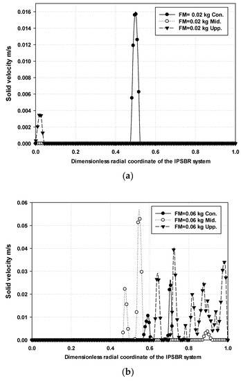
Figure 4.
Effect of mixing particle load ((a) 0.02 kg and (b) 0.06 kg) on the average solid velocity at a constant feed gas velocity of 1 m/s, orifice diameter of 0.003 m, gas head of 0.25 m, and mixing particle diameter of 0.0135 m in the conical, middle, and upper regions.
4.2. Effect of Independent Parameters on the Average Solid Volume Fraction
- (a)
- Effect of feed gas velocity on the solid volume fraction
By comparing the effect of a feed gas velocity of 1.5 m/s with the effects of velocities of 1 and 0.5 m/s in all of the column regions under a constant orifice diameter of 0.003 m, gas head of 0.25 m, mixing particle diameter of 0.0135 m, and total mass of mixing particles of 0.06 kg, it was found that the maximum solid volume fraction was 0.043 in the conical region at a feed gas velocity of 1.0 m/s. When the feed gas velocity was reduced to 0.5 m/s, the majority of the particles congregated at the reactor’s bottom. This is evident in Figure 5a, which shows a very low volume fraction in almost all of the regions. This is due to the fact that all of the particles were concentrated at the bottom of the reactor and moving very slowly.
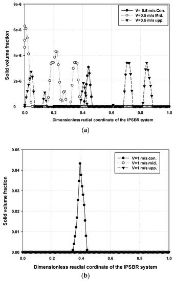
Figure 5.
Effect of feed gas velocity ((a) 0.5 m/s and (b) 1.0 m/s) on the average solid volume fraction at a constant orifice diameter of 0.003 m, gas head of 0.25 m, mixing particle diameter of 0.0135 m, and total mass of mixing particle of 0.06 kg in the conical, middle, and upper regions.
- (b)
- Effect of orifice diameter on solid volume fraction
The effect of the orifice diameter was examined under a feed gas velocity of 1 m/s, mixing particle diameter of 0.0135 m, and mixing particle load of 0.06 kg and gas head of 0.003. It was observed that as the orifice diameter was reduced from 0.005 m to 0.001 m, the volume fraction of gas phase decreased in all regions and accordingly the superficial velocity of the created bubbles inside the reactor is decreased. More circulation and eddies were also observed because of increasing gas residence time inside the system. This enhanced the surface contacted between the three phases along the reactor.
- (c)
- Influence of gas head on solid volume fraction
Figure 6a,b demonstrates an overview of the change in the solid volume fraction with respect to the gas head (0.15 and 0.35 m) at a feed gas velocity of 1 m/s, orifice diameter of 0.003 m, mixing particle diameter of 0.0135 m, and total mass of mixing particle of 0.06 kg in all three regions. It was observed that by decreasing the gas head (more gas holdup) from 0.35 to 0.15, the solids concentration decreased throughout the reactor. The solid volume fraction at R = 0.55 m and a gas head of 0.15 m was around 1.2 × 10⁻⁶ in the upper region. For a gas head of 0.35 at the same position (R = 0.55) m, the solid volume fraction approached the value of 2.3 × 10⁻⁶ in the upper region.
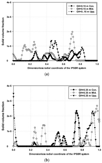
Figure 6.
Effect of gas head ((a) 0.15 m and (b) 0.35 m) on the average solid volume fraction at a constant feed gas velocity of 1 m/s, orifice diameter of 0.003 m, mixing particle diameter of 0.0135 m, and total mass of mixing particle of 0.06 kg/s in the conical, middle, and upper regions.
- (d)
- Effect of mixing particle diameter on solid volume fraction
The effect of particle size could not be separated from the effect of the solids concentration. It was concluded that deceasing the particle size from 0.0225 to 0.0135 could increase the solid volume fraction in the conical region. Where increasing the particle size resulted in a high precipitation of solids at the bottom of the reactor. This is illustrated in Figure S3a,b for a particle size of 0.0135 and 0.0225 m under a constant feed gas velocity of 1 m/s, orifice diameter of 0.003 m, gas head of 0.25 m, and total mass of mixing particle of 0.06 kg in all three regions. Selecting the proper particle diameter is very important for ensuring a uniform distribution of particles along the reactor. This will enhance the interfacial areas between the gas and liquid, and also improve the gas holdup and thus the overall performance of the reactor.
- (e)
- Effect of mixing particle load on solid volume fraction
It was noted that when the particle load increased from 0.02 kg to 0.1 kg, the solid volume fraction increased from 3 × 10⁻⁵ to 0.045, especially in the conical region. This enhanced the contact area between the gas and liquid in the middle and upper regions. However, in the conical region, increasing the volume fraction enhanced the bubble coalescence and accordingly decreased the gas holdup owing to the small cross-sectional area compared to the middle and upper regions, as was also observed by other reporters [39].
4.3. Influences of Factors on the Mass Concentration of Mixing Particles
Based on the RSM responses, a polynomial equation (second order) in terms of dependent and significant independent coded variables for the three regions is given by Equations (12)–(14), respectively.
Particle mass concentration (Con.) [kg/cm3] = −55.87 + 24.10 V + 6044 OD + 170.3 GH + 1384 DM + 254.7 FM − 11.73 V2 − 801,540 OD2 − 313.0 GH2 − 43,206 DM2 − 2099 FM2 − 931 V OD − 1.6 V GH + 95 V DM + 37.7 V FM + 939 OD GH − 18,689 OD DM − 8095 OD FM − 951 GH DM − 32 GH FM − 57 DM FM
Particle mass concentration (Mid) [kg/cm3] = 12.942 − 5.911 V − 2130 OD − 58.78 GH + 314.6 DM − 68.77 FM + 2.588 V2 + 280,405 OD2 + 61.40 GH2 + 755 DM2 + 17.5 FM2 − 81.1 V OD + 15.84 V*GH − 156.6 V DM + 3.85 V FM − 435 OD GH + 36,716 OD DM − 1747 OD FM − 567.6 GH DM + 396.8 GH FM − 2381 DM FM
Particle mass concentration (Upp.) [kg/cm3] = 2.29 + 3.01 V − 1210 OD − 21.06 GH + 381.3 DM − 81.5 FM + 0.642 V2 + 314,512 OD2 + 61.0 GH2 + 1482 DM2 + 612.2 FM2 − 1443 V OD + 21.20 V GH − 248.6 V DM − 44.62 V FM − 3613 OD GH + 73,183 OD DM + 17,861 OD FM − 1672 GH DM − 0.1 GH FM + 1074 DM FM
Table 3 and Table S1 show the results obtained from the regression model for the solid mass concentration in the middle and upper regions, respectively. The p-values were low (˂0.05) for most of the interactions, which is an indication of the high significance of the model as reported by others [38,39,40]. Moreover, the regression model had a high value of R2, which was 99.68% for the middle region and 98.50% for the upper region.
Table 3.
ANOVA analysis for average middle particle mass concentration.
Pareto plots for the middle, upper, and conical regions were used to detect the most significant factors and interactions that affect the solid mass concentration. It was found that most of the main effects and two-factor interactions are statistically significant at a 5% significance level. It is also worth mentioning that the normal plots indicate that the residuals fall approximately in a straight line, which provides further confirmation of the acceptability of the model.
4.4. Influences of Factors on Average Solid Volume Fraction
The ANOVA analysis for the average solid volume fraction in the middle region is provided in Table S2. It shows that all of the linear and quadratic coefficients are significant (p > 0.05). The exception is the two-way interactions between the orifice diameter and mixing particle load. This is according to the p-values, which are greater than 0.05. Moreover, the R2 had a high value of 0.9961. The adequacy of the results for the conical, middle, and upper regions was confirmed by residual analysis, and the transformed data in the normal probability results were found to be very close to the normality distribution curves. Furthermore, the residuals-versus-order fluctuations revealed that there is no pattern, indicating independence. All of the collected data showed a good distribution of the CFD-simulated data and predicted values, with no differences observed.
4.5. Influences of Factors on Average Mixing Particle Velocity
The second-order polynomial regression equations indicating the mixing particle velocity are expressed by Equations (15)–(17) for the three regions of the system, respectively:
Conical solid velocity [m/s] = −0.12564 + 0.10226 V + 28.51 OD − 0.4387 GH + 9.788 DM + 1.1276 FM − 0.05986 V2 − 3275 OD2 + 0.7234 GH2 − 200.12 DM2 − 9.575 FM2 − 6.746 V OD + 0.1609 V GH − 0.026 V DM + 0.0059 V FM − 15.89 OD GH − 263.7 OD DM + 59.33 OD FM − 5.508 GH DM + 1.239 GH FM − 35.78 DM FM
Middle solid velocity [m/s] = 0.10768 − 0.07098 V − 8.91 OD − 0.7358 GH + 6.722 DM − 0.4310 FM + 0.01074 V2 + 631.2 OD2 + 1.1561 GH2 + 3.63 DM2 + 5.444 FM2 + 3.216 V OD + 0.3102 V GH − 1.060 V DM − 0.2796 V FM + 17.23 OD GH − 611.9 OD DM + 73.70 OD FM − 10.323 GH DM − 0.390 GHFM − 20.53 DMFM
Upper solid velocity [m/s] = 0.08385 − 0.01650 V − 11.27 OD − 0.7723 GH + 6.179 DM − 0.1158 FM + 0.00325 V2 + 1005 OD2 + 1.3412 GH2 + 46.69 DM2 + 1.181 FM2 − 2.333 V*OD + 0.2618 V*GH − 2.249 V*DM − 0.3501 V*FM + 7.71 OD*GH − 117.6 OD*DM + 134.92 OD*FM − 14.809 GH*DM + 0.026 GH*FM − 10.61 DM*FM
The Pareto analysis, which reveal the most important factors influencing the average mixing particle velocity in all three regions, was carried out and exposed that most of the parameters had a great impact on the responses. These results were confirmed from the p-value, which is less than 0.05 for most of the factors, and the R2, which is very close to 1. The residual normal probability analysis for the solid velocity indicates that all of the residuals fall around a line, with no obvious outliers or scattering.
4.6. Response Optimizer
In this study, three responses (mass concentration of mixing (R1–R3), average solid volume fraction (R4–R6) and average mixing particle velocity (R7–R9)) are calculated. It is desirable to find the maximum values of these three responses in the middle and upper regions. However, in the conical region it is desirable to find their low values. In the conical region, most of the particles will have settled and it is important to minimize the concentration of solids and turbulence in this region by setting the velocity and concentration to a minimum (Table S3). This will reduce the coalescence between the bubbles and increase the gas holdup in the region. In order to ensure a good distribution of particles in the middle and upper regions, the values of solid velocity and concentration should be at their maximum. This will increase the interfacial areas between particles, gas, and liquid. It will also enhance the residence time of the process.
In our previous work [13], the desirable upper, middle, and conical air volume fractions (R10–R12) were considered and targeted to be maximum to achieve maximum interfacial area concentration, whereas the desirable upper, middle, and conical air velocities (R13–R15) were studied and targeted to be minimal to achieve maximum gas residence time. The optimizer prediction shows that the lowest average air velocity and highest average air volume fraction in the conical, middle, and upper regions were achieved at feed-gas velocity of 1.5 m/s, gas head of 0.164 m, orifice diameter of 0.001 m, mixing-particle diameter of 0.0225 m, and total mass of mixing-particle of 0.02 kg as demonstrated in Table S4.
In this work, all preceding responses (R1–R15) were combined together and optimized using the Minitab response optimizer conferring to the stated targets to have a wider indication for the hydrodynamic performance for the IPSBR system. The optimal parameters were found to be a feed gas velocity of 1.5 m/s, orifice diameter of 0.001 m, gas head of 0.202 m, mixing particle diameter of 0.0107 m, and total mass of mixing particles of 0.02 kg. The optimization outcomes are listed in Table 4. Remarkably, for the same optimal parameters, a high air volume fraction and low air velocity were attained. This result reflects the novelty of the IPSBR, which can operate at high feed gas velocities while maintaining a high gas residence time and high gas volume fraction. The overall desirability is assessed as one, which specifies that the response optimization is satisfactory [41,42]. When comparing Table S4 and Table 4, operational conditions in the same range were observed, confirming the same physical concept of achieving high contact surface area, gas residence time, and mixing particle distribution at the specified operational conditions range.
Table 4.
Optimum conditions and simulated fitted responses with composite desirability of one.
4.7. Validation of the CCD Model
The optimal operational conditions of feed gas velocity 1.5 m/s, orifice diameter 0.001 m, gas head 0.202 m, mixing particle diameter 0.0107 m, and mixing particle load of 0.02 kg were entered into the ANSYS software model to collect all predicted responses (R1–R15). The predicted responses from the regression model were found to agree with those obtained from the simulated data, which confirmed the model’s validity and adequacy, as shown in Table 5. The predicted and simulated responses are very close and within the 95 percent confidence interval, indicating that the model can predict the hydrodynamic performance of the simulated IPSBR system under various operational conditions.
Table 5.
Results of validation tests for CCD design and optimizer outputs.
Solid velocity, mass concentration, and eddies viscosities were plotted to visualize the effect of the optimum conditions on the dispersion of the mixing particles throughout the system region, as shown in Figure 7a at feed gas velocity of 0.5 m/s, orifice diameter of 0.003 m, gas head of 0.25 m, mixing particle diameter of 0.018 m, and total mass of mixing particle of 0.04 kg. These results were compared at the optimum condition, Figure 7b, with a feed gas velocity of 1.5 m/s, orifice diameter of 0.001 m, gas head of 0.202 m, mixing particle diameter of 0.0107 m, and total mixing particle mass of 0.02 kg. It was clear that the optimized condition exhibits uniform eddies viscosity distribution, velocity and mass concentration among the three regions, and thus better mixing particle dispersion is expected. In addition, the swirling motion, which is detected in Figure 7b, affects the particle movement as it pushes particles in fluid movement direction. This may lead to larger residence time for the fluid due to the circulation zone [43].
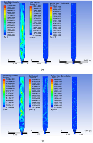
Figure 7.
Solid eddies, velocities, and particle mass concentration contours over the three regions (a) at 0.5 m/s feed gas velocity, 0.003 m orifice diameter, 0.25 m gas head, 0.018 m mixing particle diameter, and 0.04 kg total mixing particle mass and (b), with a feed gas velocity of 1.5 m/s, an orifice diameter of 0.001 m, a gas head of 0.202 m, a mixing particle diameter of 0.0107 m, and a total mass of 0.02 kg.
4.8. Contour Plots
Figure 8a–d depicts the effect of feed gas velocity and orifice diameter on the average solid velocity and solid volume fraction in the contact system’s conical and middle regions. The contours show that increasing the feed gas velocity (to nearly 1.5 m/s) and decreasing the orifice diameter (to 0.001 m) are important in maximizing the solid velocity and volume fraction in the middle region.

Figure 8.
(a,b) average middle solid velocity and solid volume fraction (c,d) on 2D plots as a function of feed gas velocity and orifice diameter.
Figure S4a,b demonstrates that the maximum solid volume fraction in the conical and upper region can be obtained at a gas head value of nearly 0.24 m and at a low particle diameter value.
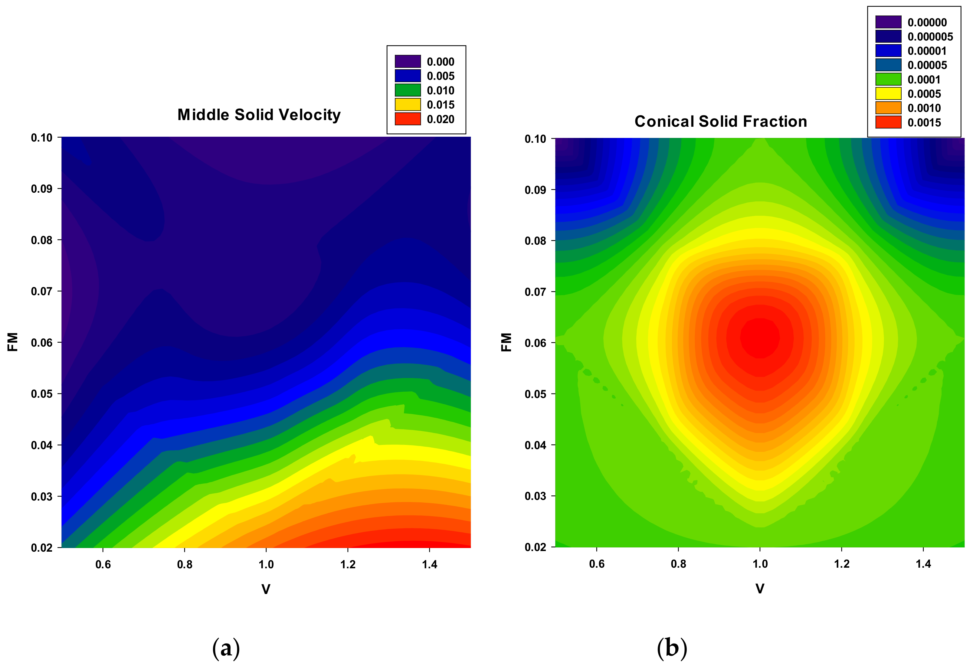
From Figure 9a, it is clear that the feed gas velocity and particle load had a significant impact on the solid velocity in the middle region of the reactor. By increasing the feed gas velocity and decreasing the particle load can maximize the solid velocity at this region. However, at the same parameter conditions, the solid volume fraction reached its minimum value in the conical region as shown in Figure 9b.

Figure 9.
(a) middle solid velocity and (b) conical solid fraction on 2D plots as a function of feed gas velocity and mixing particle load.
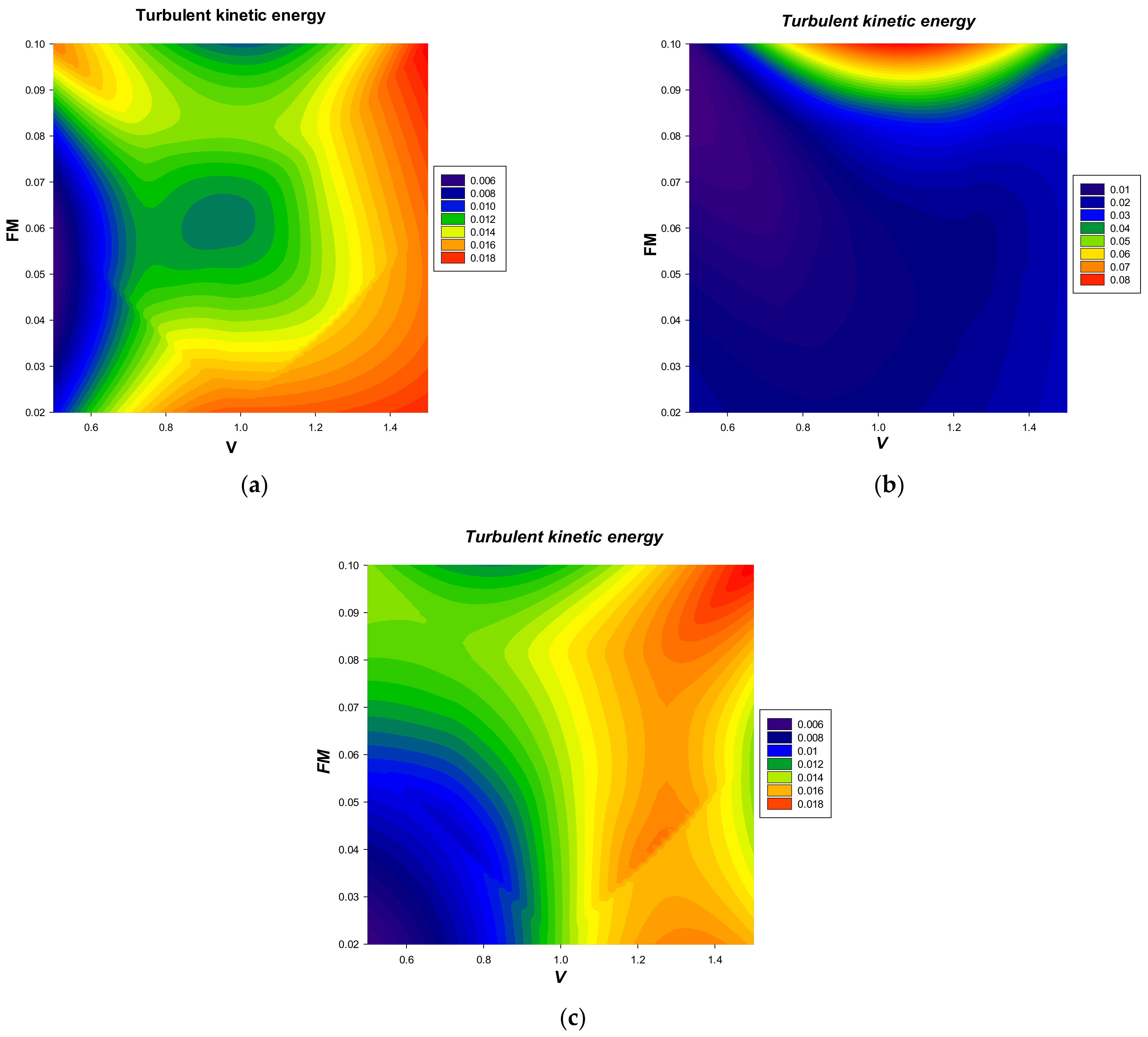
As mentioned in Section 4.1 (c), the effect of particle dispersion on turbulence in the three system zones is significant. Figure 10a–c depicts the change in turbulent kinetic energy as a function of feed gas velocity and total mass of the mixing particles. The turbulent kinetic energy was found to be significantly higher in the conical and upper regions than in the middle region. Since particles are injected into the conical region and gas bubbles are generated through an orifice, large turbulences and disturbances are likely to occur. Similarly, high turbulences can be expected in the upper region where bubbles exit the liquid phase and enter the gas outlet from the reactor’s top.

Figure 10.
(a) conical, (b) middle, and (c) average upper turbulent kinetic energy on 2D plots as a function of feed gas velocity and total mass of mixing particles.
4.9. Validation of the CFD Model
Many studies have investigated the hydrodynamics of conical-base spouted bed based on 2-dimentional axisymmetric geometry assumption using the CFD–DEM coupling approach [4,44,45,46,47,48], and based on the conventional gas–solid or gas–liquid spouted bed phenomena. The novelty of the current research is to investigate the performance of inert-particle spouted bed reactor (IPSBR) system with three-phase mixture (liquid, gas, and solid).
It is important to note that the fluid movement simulation obtained by solving the Navier–Stokes equation is always correct for the fluid domain for the given operating conditions. The location of the solid particles may vary based on its location in the axisymmetric plan. Accordingly, the results obtained from the studied model are valid if the particles are located in the radial location. However, the particles may not always be present in the same location around the axisymmetric plan, then caution should be stressed that the axisymmetric assumption is valid for the fluid domain and not for the particles in the Lagrangian model [49,50]. An experimental validation for the tested model would show us the deviation on simulated data based on the previous assumption and will be compared with the reported data.
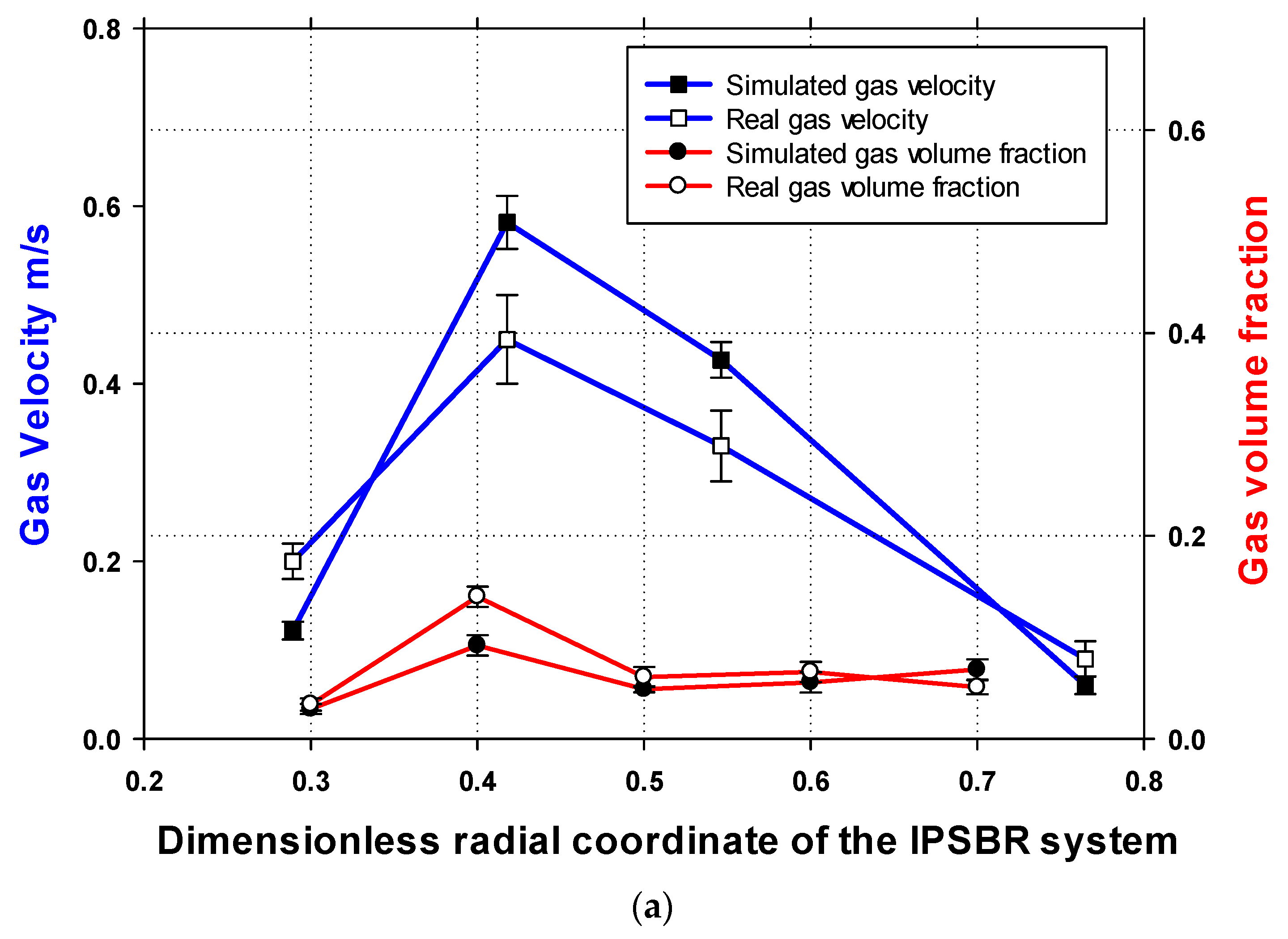
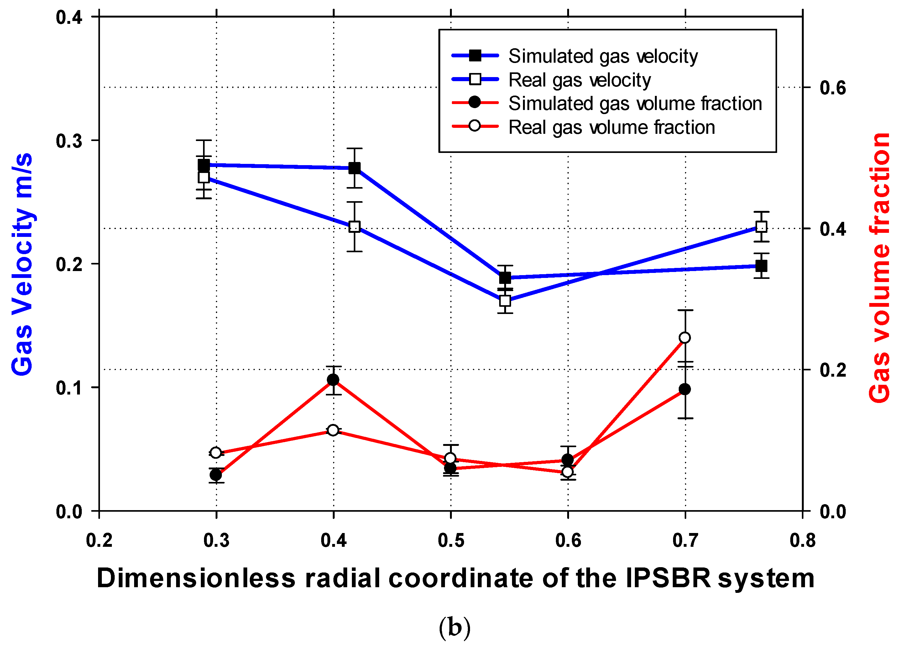
A laboratory-scale IPSBR system with the same geometry as that considered in previous studies [13,14] was utilized to validate the Eulerian model. Spherical acrylic particles with a diameter of 0.005 m was used. A gas orifice (ID of 0.002 m) is located at the center of the bottom plate for gas injection. The validation runs considered the presence and absence of mixing particles. A high-speed digital video camera was used to collect measurements reflecting bubbles characteristics, such as the velocity, trajectories, and diameter. The bubble velocity and volume fraction was measured in the radial direction and vertically using Photron FASTCAM Viewer software (PFV) Ver. 3282. Figure 11 shows the simulated and experimental results at specific height from the gas inlet (50 mm) for gas velocity and volume fraction in the two cases: with and without mixing particles. The detected alteration in velocities and volume fractions values are in good agreement with the CFD-simulated data and with an acceptable deviation as listed in Table 2. Still, as reported by Ekambara et al. [31], the 3D model is the only model that could closely predict the experimental data for the majority of the three-phase system. However, the proposed 2D model showed a good and simple estimation with an acceptable deviation between the simulated and experiment data (5–10%), as confirmed in Table 6. Table 7 summarizes the main findings from the current research and compares them with validated results from the literature.
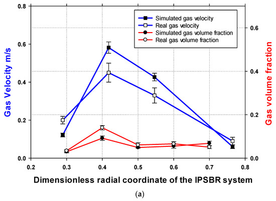
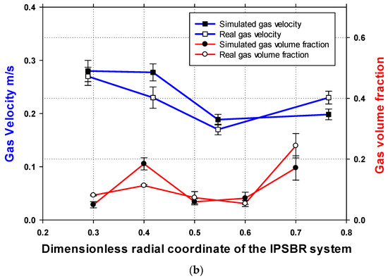
Figure 11.
Experimental and simulation results at certain points for air velocity and air volume fraction (a) with mixing particles and (b) without mixing particles.
Table 6.
Experimental and simulated average gas velocity and volume fraction with and without mixing particles and calculated error deviation (5–10%).
Table 7.
Summary of some CFD validated results studied based on 2-dimentional axisymmetric assumption.
5. Conclusions
RSM was implemented to assess the effects of feed gas velocity, orifice diameter, gas head, mixing particle diameter, and particle load on the average solid volume fraction, mass concentration of mixing particles, and average mixing particle velocity, which was produced from the CFD results of the novel IPSBR system. The best conditions were a feed gas velocity of 1.5 m/s, orifice diameter of 0.001 m, gas head of 0.2025 m, particle diameter of 0.0107 m, and particle load of 0.02 kg. A good distribution of particles throughout the reactor was observed under these conditions. It was also observed that the maximum air volume fraction and minimum air velocity from the previous work occurred inside the reactor under the same feed gas velocity of 1.5 m/s, orifice diameter of 0.001 m and total mass particles of 0.02, and with very similar gas head and particle diameter values. This was a significant confirmation of the novelty of the reactor, as it could achieve a high gas holdup, high residence time, and good particle distribution under the maximum feed gas velocity value of 1.5 m/s.
Supplementary Materials
The following are available online at https://www.mdpi.com/article/10.3390/pr9111921/s1, Figure S1: Effect of orifice diameter ((a) 0.003 m, and (b) 0.005 m) on the average solid velocity at a constant feed gas velocity of 1m/s, gas head of 0.25 m, mixing particle diameter of 0.0135 m, and total mass of mixing particle of 0.06 kg in the conical, middle, and upper regions, Figure S2: Effect of mixing particle diameter ((a) 0.0135 m, (b) 0.0225 m) on average solid velocity at a constant feed gas velocity of 1 m/s, orifice diameter of 0.003 m, gas head of 0.25 m, and total mass of mixing particle of 0.06 kg in the conical, middle, and upper regions, Figure S3: Effect of mixing particle diameter ((a) 0.0135 m and (b) 0.0225 m) on the average solid volume fraction at a constant feed gas velocity of 1 m/s, orifice diameter of 0.003 m, gas head of 0.25 m, and total mass of mixing particle of 0.06 kg/s in the conical, middle, and upper regions, Table S1: ANOVA analysis for average upper particle mass concentration, Table S2: ANOVA analysis for average middle solid volume fraction, Table S3: Optimization setting for particle mass concentration, solid volume fraction, solid velocity, air velocity, and air volume fraction, Table S4: Optimum conditions and fitted responses with composite desirability of one [8]. Figure S4: Average conical and upper solid volume fraction on 2D plots for response surface optimization versus particle diameter and gas head.
Author Contributions
Conceptualization, A.F.M., A.A.-H.I.M., A.H.A.-M., M.H.E.-N., B.V.d.B. and M.H.A.-M.; methodology, A.F.M. and F.A.; software, A.F.M.; formal analysis, A.F.M. and A.A.-H.I.M.; investigation, A.H.A.-M., M.H.E.-N., B.V.d.B. and M.H.A.-M.; resources, A.H.A.-M., M.H.E.-N. and M.A.M.; writing—original draft preparation, A.F.M. and A.A.-H.I.M.; writing—review and editing, A.A.-H.I.M., A.H.A.-M., M.H.E.-N., B.V.d.B. and M.H.A.-M.; supervision, A.H.A.-M., M.H.E.-N., B.V.d.B. and M.H.A.-M.; project administration, A.H.A.-M., M.H.E.-N. and M.A.M.; funding acquisition, A.H.A.-M. and M.A.M. All authors have read and agreed to the published version of the manuscript.
Funding
This research was funded by the ADNOC Refining Research Center, Abu Dhabi, United Arab Emirates, grant number 21N224, https://dx.doi.org/10.13039/501100002672 (accessed on 20 September 2021).
Acknowledgments
The authors would like to express their sincere gratitude to Jawad Mustafa from Chemical Engineering Department at the UAE University for his valuable help and assistance.
Conflicts of Interest
The authors certify that they have no conflicts of Interest in the subject matter or materials discussed in this manuscript.
Nomenclature
| Roman letters | |
| Drag coefficient | |
| Particle diameter (m) | |
| 2DD | Two dimensional |
| Drag force (N) | |
| g | Gravity (m/s2) |
| Momentum exchange coefficient between qth and kth phases | |
| Interphase exchange forces | |
| Reynolds number | |
| Latin letters | |
| Tensor notation for velocity in i direction | |
| Tensor notation for velocity in j direction | |
| Tensor notation for space coordinates | |
| , | Turbulence model constants |
| Greek letters | |
| kth phase stress–strain tensor | |
| Average mixture velocity (gas and liquid) | |
| Fluid velocity for th phase (m/s) | |
| Abbreviations | |
| CFD | Computational fluid dynamics |
| CCD | Central composite design |
| CO2 | Carbon dioxide |
| CSTR | Continuous stirred-tank reactor |
| DM | Diameter of mixing particle |
| DPM | Discrete phase mode |
| FM | Mixing particle load |
| GH | Gas head |
| IPSBR | Inert-particles spouted-bed reactor |
| OD | Orifice diameter |
| PBM | Population balance model |
| RSM | Response surface methodology |
| Fluid velocity for th phase (m/s) | |
| Mixture molecular viscosity (Pa·s) | |
| Eddy viscosity (Pa·s) | |
| Density for phase (kg/m3) | |
| Mixture density (kg/m3) | |
| Particle density(kg/m3) | |
| K | Turbulence energy |
| ɛ | Isotropic turbulence dissipation rate |
| Particle velocity (m/s) | |
| Molecular viscosity for th phase (Pa·s) | |
| Diffusion Prandtl number for turbulence energy | |
| Diffusion Prandtl number for dissipation rate | |
References
- Konduri, R.K.; Altwicker, E.R.; Morgan, M.H., III. Design and scale-up of a spouted-bed combustor. Chem. Eng. Sci. 1999, 54, 185–204. [Google Scholar] [CrossRef]
- Jono, K.; Ichikawa, H.; Miyamoto, M.; Fukumori, Y. A review of particulate design for pharmaceutical powders and their production by spouted bed coating. Powder Technol. 2000, 113, 269–277. [Google Scholar] [CrossRef]
- Zhao, X.-L.; Li, S.; Liu, G.-Q.; Yao, Q.; Marshall, J.-S. DEM simulation of the particle dynamics in two-dimensional spouted beds. Powder Technol. 2008, 184, 205–213. [Google Scholar] [CrossRef]
- Kim, M.; Na, J.; Park, S.; Park, J.-H.; Han, C. Modeling and validation of a pilot-scale aqueous mineral carbonation reactor for carbon capture using computational fluid dynamics. Chem. Eng. Sci. 2018, 177, 301–312. [Google Scholar] [CrossRef]
- Pietsch, S.; Kieckhefen, P.; Heinrich, S.; Müller, M.; Schönherr, M.; Jäger, F.K. CFD-DEM modelling of circulation frequencies and residence times in a prismatic spouted bed. Chem. Eng. Res. Des. 2018, 132, 1105–1116. [Google Scholar] [CrossRef]
- He, Y.-L.; Qin, S.-Z.; Lim, C.J.; Grace, J.R. Particle velocity profiles and solid flow patterns in spouted beds. Can. J. Chem. Eng. 1994, 72, 561–568. [Google Scholar] [CrossRef]
- José, M.J.S.; Olazar, M.; Alvarez, S.; Izquierdo, M.A.; Bilbao, J. Solid cross-flow into the spout and particle trajectories in conical spouted beds. Chem. Eng. Sci. 1998, 53, 3561–3570. [Google Scholar] [CrossRef]
- Zhao, X.-L.; Yao, Q.; Li, S.-Q. Effects of draft tubes on particle velocity profiles in spouted beds. Chem. Eng. Technol. 2006, 29, 875–881. [Google Scholar] [CrossRef]
- Norman, E.; Grace, J.R. Spouted and Spout-Fluid Beds: Fundamentals and Applications; Cambridge University Press: Cambridge, UK, 2010. [Google Scholar]
- El-Naas, M.H.; Mohammad, A.F.; Suleiman, M.I.; Al Musharfy, M.; Al-Marzouqi, A.H. Evaluation of a novel gas-liquid contactor/reactor system for natural gas applications. J. Nat. Gas Sci. Eng. 2017, 39, 133–142. [Google Scholar] [CrossRef]
- El-Naas, M.H. System for Contacting Gases and Liquids. U.S. Patent No. 9,724,639, 8 August 2017. [Google Scholar]
- Mustafa, J.; Mourad, A.A.-H.I.; Al-Marzouqi, A.H.; El-Naas, M.H. Simultaneous treatment of reject brine and capture of carbon dioxide: A comprehensive review. Desalination 2020, 483, 114386. [Google Scholar] [CrossRef]
- Mohammad, A.F.; Mourad, A.A.-H.I.; Mustafa, J.; Al-Marzouqi, A.H.; El-Naas, M.H.; Al-Marzouqi, M.; Alnaimat, F.; Suleiman, M.I.; Al Musharfy, M.; Firmansyah, T. Computational fluid dynamics simulation of an Inert Particles Spouted Bed Reactor (IPSBR) system. Int. J. Chem. React. Eng. 2020, 18. [Google Scholar] [CrossRef]
- Mohammad, A.; Mourad, A.A.-H.I.; Al-Marzouqi, A.; El-Naas, M.H.; Van der Bruggen, B.; Al-Marzouqi, M.; Alnaimat, F.; Suleiman, M.; Al Musharfy, M. CFD and statistical approach to optimize the average air velocity and air volume fraction in an inert-particles spouted-bed reactor (IPSBR) system. Heliyon 2021, 7, e06369. [Google Scholar] [CrossRef] [PubMed]
- Su, W.; Shi, X.; Wu, Y.; Gao, J.; Lan, X. Simulation on the effect of particle on flow hydrodynamics in a slurry bed. Powder Technol. 2019, 361, 1006–1020. [Google Scholar] [CrossRef]
- Yancheshme, A.A.; Zarkesh, J.; Rashtchian, D.; Anvari, A. CFD simulation of hydrodynamic of a bubble column reactor operating in churn-turbulent regime and effect of gas inlet distribution on system characteristics. Int. J. Chem. React. Eng. 2016, 14, 213–224. [Google Scholar] [CrossRef]
- Lakhdissi, E.M.; Soleimani, I.; Guy, C.; Chaouki, J. Simultaneous effect of particle size and solid concentration on the hydrodynamics of slurry bubble column reactors. AIChE J. 2020, 66, e16813. [Google Scholar] [CrossRef]
- Sasaki, S.; Uchida, K.; Hayashi, K.; Tomiyama, A. Effects of particle concentration and slurry height on gas holdup in a slurry bubble column. J. Chem. Eng. Jpn. 2016, 49, 824–830. [Google Scholar] [CrossRef]
- Rabha, S.; Schubert, M.; Hampel, U. Intrinsic flow behavior in a slurry bubble column: A study on the effect of particle size. Chem. Eng. Sci. 2013, 93, 401–411. [Google Scholar] [CrossRef]
- Kim, Y.H.; Tsutsumi, A.; Yoshida, K. Effect of particle size on gas holdup in three-phase reactors. Sadhana 1987, 10, 261–268. [Google Scholar] [CrossRef]
- Jamialahmadi, M.; Müller-Steinhagen, H. Effect of solid particles on gas hold-up in bubble columns. Can. J. Chem. Eng. 1991, 69, 390–393. [Google Scholar] [CrossRef]
- Ojima, S.; Sasaki, S.; Hayashi, K.; Tomiyama, A. Effects of particle diameter on bubble coalescence in a slurry bubble column. J. Chem. Eng. Jpn. 2015, 48, 181–189. [Google Scholar] [CrossRef]
- Gholamzadehdevin, M.; Pakzad, L. Hydrodynamic characteristics of an activated sludge bubble column through computational fluid dynamics (CFD) and response surface methodology (RSM). Can. J. Chem. Eng. 2019, 97, 967–982. [Google Scholar] [CrossRef]
- Pashaei, H.; Ghaemi, A.; Nasiri, M.; Karami, B. Experimental modeling and optimization of CO2 absorption into piperazine solutions using RSM-CCD methodology. ACS Omega 2020, 5, 8432–8448. [Google Scholar] [CrossRef] [Green Version]
- Song, C.; Kitamura, Y.; Li, S. Optimization of a novel cryogenic CO2 capture process by response surface methodology (RSM). J. Taiwan Inst. Chem. Eng. 2014, 45, 1666–1676. [Google Scholar] [CrossRef] [Green Version]
- Batchelor, G.K. An Introduction to Fluid Dynamics; Cambridge University Press: Cambridge, UK, 1967. [Google Scholar]
- Launder, B.E.; Spalding, D.B. Lectures in Mathematical Models of Turbulence; Academic Press: London, UK, 1972. [Google Scholar]
- Lam, C.K.G.; Bremhorst, K. A Modified form of the k-ε model for predicting wall turbulence. J. Fluids Eng. 1981, 103, 456–460. [Google Scholar] [CrossRef]
- Morsi, S.A.; Alexander, A.J. An investigation of particle trajectories in two-phase flow systems. J. Fluid Mech. 1972, 55, 193–208. [Google Scholar] [CrossRef]
- Ekambara, K.; Dhotre, M.T.; Joshi, J.B. CFD simulations of bubble column reactors: 1D, 2D and 3D approach. Chem. Eng. Sci. 2005, 60, 6733–6746. [Google Scholar] [CrossRef]
- Aghbolaghy, M.; Karimi, A. Simulation and optimization of enzymatic hydrogen peroxide production in a continuous stirred tank reactor using CFD–RSM combined method. J. Taiwan Inst. Chem. Eng. 2014, 45, 101–107. [Google Scholar] [CrossRef]
- Myers, R.H.; Montgomery, D.C.; Anderson-Cook, C.M. Process and product optimization using designed experiments. Response Surf. Methodol. 2002, 2, 328–335. [Google Scholar]
- Ölmez, T. The optimization of Cr (VI) reduction and removal by electrocoagulation using response surface methodology. J. Hazard. Mater. 2009, 162, 1371–1378. [Google Scholar] [CrossRef]
- Körbahti, B.K.; Rauf, M. Application of response surface analysis to the photolytic degradation of Basic Red 2 dye. Chem. Eng. J. 2008, 138, 166–171. [Google Scholar] [CrossRef]
- Kim, K.-Y.; Seo, J.-W. Shape optimization of a mixing vane in subchannel of nuclear reactor. J. Nucl. Sci. Technol. 2004, 41, 641–644. [Google Scholar] [CrossRef]
- Bouaifi, M.; Hebrard, G.; Bastoul, D.; Roustan, M. A comparative study of gas hold-up, bubble size, interfacial area and mass transfer coefficients in stirred gas–liquid reactors and bubble columns. Chem. Eng. Process. Process Intensif. 2001, 40, 97–111. [Google Scholar] [CrossRef]
- Rabha, S.; Schubert, M.; Wagner, M.; Lucas, D.; Hampel, U. Bubble size and radial gas hold-up distributions in a slurry bubble column using ultrafast electron beam X-ray tomography. AIChE J. 2012, 59, 1709–1722. [Google Scholar] [CrossRef]
- Gao, Y.-L.; Ju, X.-R. Statistical prediction of effects of food composition on reduction of Bacillus subtilis As 1.1731 spores suspended in food matrices treated with high pressure. J. Food Eng. 2007, 82, 68–76. [Google Scholar] [CrossRef]
- Zhao, H.; Hu, H.-R. Optimal design of a pipe isolation plugging tool using a computational fluid dynamics simulation with response surface methodology and a modified genetic algorithm. Adv. Mech. Eng. 2017, 9. [Google Scholar] [CrossRef]
- Antony, J. Design of Experiments for Engineers and Scientists; Elsevier: Amsterdam, The Netherlands, 2014. [Google Scholar]
- Unal, O. Optimization of shot peening parameters by response surface methodology. Surf. Coat. Technol. 2016, 305, 99–109. [Google Scholar] [CrossRef]
- Szafran, R.G.; Kmieć, A.; Ludwig, W. CFD modeling of a spouted-bed dryer hydrodynamics. Dry. Technol. 2005, 23, 1723–1736. [Google Scholar] [CrossRef]
- Shi, H.; Reza, O.; Nikrityuk, P.A. The impact of swirling on the dynamics of a spouted bed. Powder Technol. 2020, 380, 143–151. [Google Scholar] [CrossRef]
- Yang, S.; Luo, K.; Fang, M.; Fan, J. CFD-DEM simulation of the spout-annulus interaction in a 3D spouted bed with a conical base. Can. J. Chem. Eng. 2014, 92, 1130–1138. [Google Scholar] [CrossRef]
- Duarte, C.; Olazar, M.; Murata, V.; Barrozo, M. Numerical simulation and experimental study of fluid–particle flows in a spouted bed. Powder Technol. 2009, 188, 195–205. [Google Scholar] [CrossRef]
- Rong, L.-W.; Zhan, J.-M. Improved DEM-CFD model and validation: A conical-base spouted bed simulation study. J. Hydrodyn. 2010, 22, 351–359. [Google Scholar] [CrossRef]
- Ren, B.; Zhong, W.; Jin, B.; Shao, Y.; Yuan, Z. Numerical simulation on the mixing behavior of corn-shaped particles in a spouted bed. Powder Technol. 2013, 234, 58–66. [Google Scholar] [CrossRef]
- Zhong, W.; Yu, A.; Liu, X.; Tong, Z.; Zhang, H. DEM/CFD-DEM modelling of non-spherical particulate systems: Theoretical developments and applications. Powder Technol. 2016, 302, 108–152. [Google Scholar] [CrossRef]
- Gidaspow, D. Multiphase Flow and Fluidization: Continuum and Kinetic Theory Descriptions, 1st ed.; Academic Press: San Diego, CA, USA, 1994; p. 207. [Google Scholar]
- Anderson, T.B.; Jackson, R. Fluid mechanical description of fluidized beds. Equations of motion. Ind. Eng. Chem. Fundam. 1967, 6, 527–539. [Google Scholar] [CrossRef]


Publisher’s Note: MDPI stays neutral with regard to jurisdictional claims in published maps and institutional affiliations. |
© 2021 by the authors. Licensee MDPI, Basel, Switzerland. This article is an open access article distributed under the terms and conditions of the Creative Commons Attribution (CC BY) license (https://creativecommons.org/licenses/by/4.0/).