1. Introduction
The core principle of aerodynamic levitation is based on suspending an arbitrary object in the air using airflow. The practical use-case of this phenomenon can be seen in applications where physical contact between objects must be avoided. It is usually utilized on a microscopic scale to prevent oxidation or crystal formation upon object contact with its container. This method allows studying materials under unusual conditions and even allows the formation of new glass materials [
1].
The goal of our design of an Aerodynamic Ball Levitation Plant is to levitate a ping-pong ball inside a tube using the stream of air produced by a fan. From a control engineering aspect, this model is interesting for its simplicity of modeling and its low price. Similar to the Magnetic Levitation Plant, which uses a magnetic force to levitate a steel ball [
2], the Aerodynamic Levitation Plant could also be a part of control engineering courses provided by the Center of Modern Control Techniques and Industrial Informatics (CMCT&II) at the Department of Cybernetics and Artificial Intelligence (DCAI), Faculty of Electrical Engineering and Informatics (FEEI), Technical University of Košice (TUKE). As the commercial availability of such plant types is limited, we opted to construct one. The main advantage of the Aerodynamic Levitation Plant over the Magnetic Levitation Plant is its slower dynamics. It allows the use of a larger sampling period and consequently more computationally expensive control algorithms. This model also provides a wider ball position operation range that makes experimental identification simpler.
Several world scientists have already worked on a similar Aerodynamic Ball Levitation Plant. The authors of [
3] focused mainly on the physical construction of the plant, the choice of the most suitable sensor for measuring the ball’s position, and its analytical modeling. Apart from the physical construction, the authors of [
4] focused more on controller design based on the experimentally identified Autoregressive model with Exogenous Variable (ARX model) in the input–output form. In this case, an Arduino Mega equipped with an ATmega2560 microcontroller was used as an analog-to-digital interface of the control computer. Others contributed mainly to the application of a nonlinear modification of the Proportional-Integral-Derivative (PID) controller in the context of the Aerodynamic Levitation Plant [
5]. Papers [
6,
7,
8] were more focused on making this type of plant available in virtual and remote laboratories and used classical controllers like the PID controller. The authors of [
9] had taken a more experimental approach in the controller design and utilized a simple switched controller inspired by the sliding window controller. Although the noise filtration and proper state estimation are purposefully left out in this design method, the designed control algorithm performed well in the simulation and on the real plant. Up to this point, all authors used airflow to levitate a ball inside a tube. A different approach was used in [
10,
11,
12], where the ball was not placed inside a tube. This arrangement is more challenging in terms of both measuring the ball’s position and the power requirements. On the other hand, the plant is inherently stable from a control engineering aspect, as the airflow speed gradually decreases over distance. The authors of [
13] presented a model-free based control algorithm design for a similar plant (the Magnetic Levitation Plant). This method uses an experimental approach to fine-tune controller parameters for a target application. Another option is to use a nonlinear state-space controller as in [
14]. This controller provides the robustness needed for systems with varying parameters. From our own experience [
2] with a similar magnetic levitation plant, we decided to start with a linear state-space controller instead of a PID controller. Although linear controllers are not as robust as their nonlinear counterparts, they are easier to design. The authors of [
15] used the exact linearization approach to design a controller for the Magnetic Levitation Plant. This method combines linear controller synthesis with nonlinear compensation. A notable drawback of this method is finding a suitable mathematical transformation that transforms the nonlinear system model into a linear one.
While facing the task of experimental identification, most authors have chosen linear approximations of a mathematical model, such as the ARX model [
4,
5,
7,
16]. From the control design aspect, this is not an issue, since they proved the ARX model to be sufficient for this application. The main limitation seen in this approach is that the nonlinear mathematical model obtained from analytical identification is more suitable for the controller verification in a simulation environment. This is the reason why the authors of [
17] opted for nonlinear parameter estimation. Their focus was to create an open-source design that can be adopted by others. Although filtration is mentioned in figures, no more information about the used filtration method is provided. Considering that noise is the natural phenomenon of all physical systems, room for improvement is present. Only [
16] utilized a low-pass filter to reduce sensory noise. There are a few papers [
5,
7,
16] that included dynamics of a fan in the mathematical model, but they did not utilize state-space control. The goal of this paper is to solve presented open problems, mainly the parameter identification of the mathematical model, noise filtration, and utilization of the state-space control.
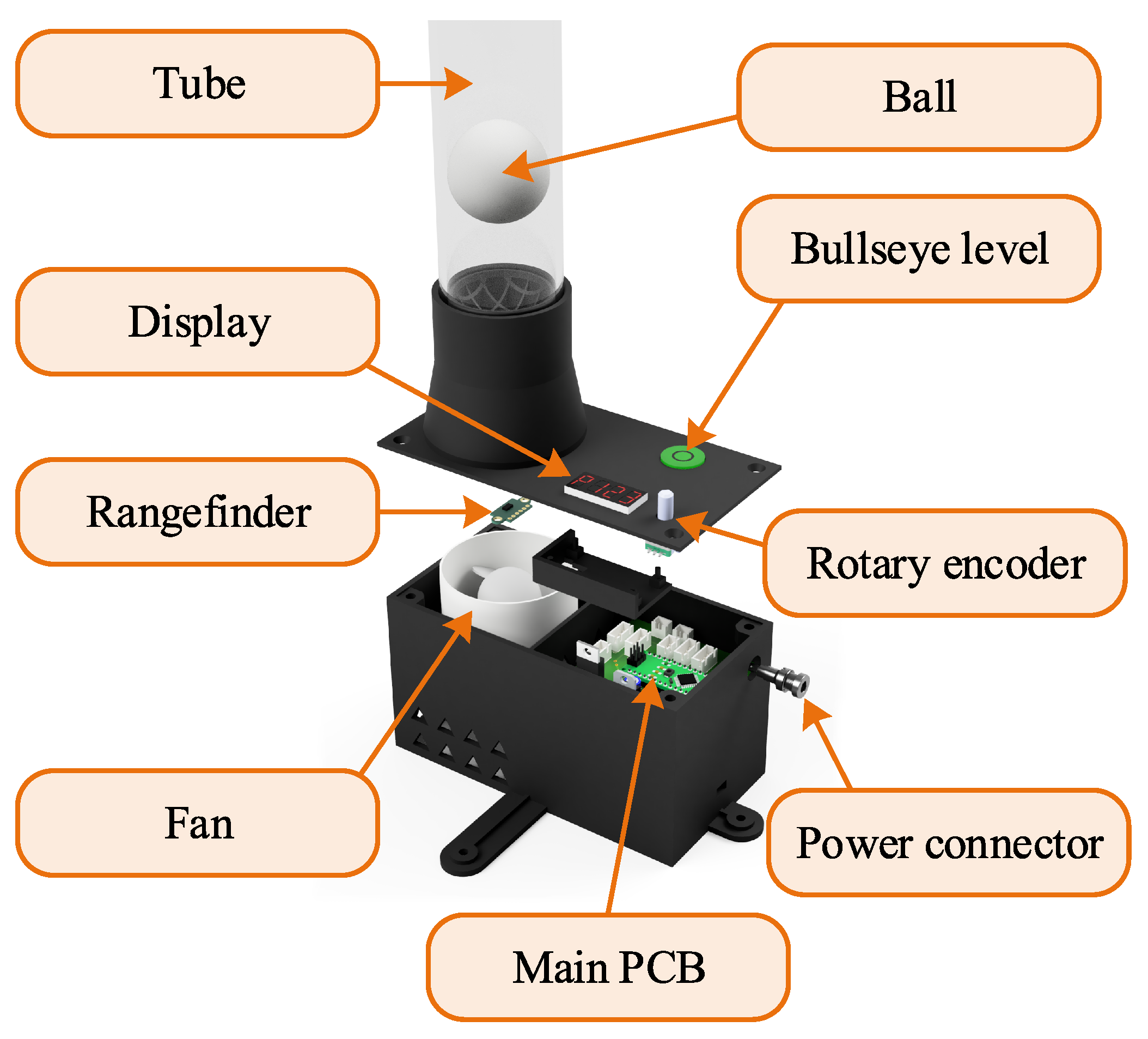
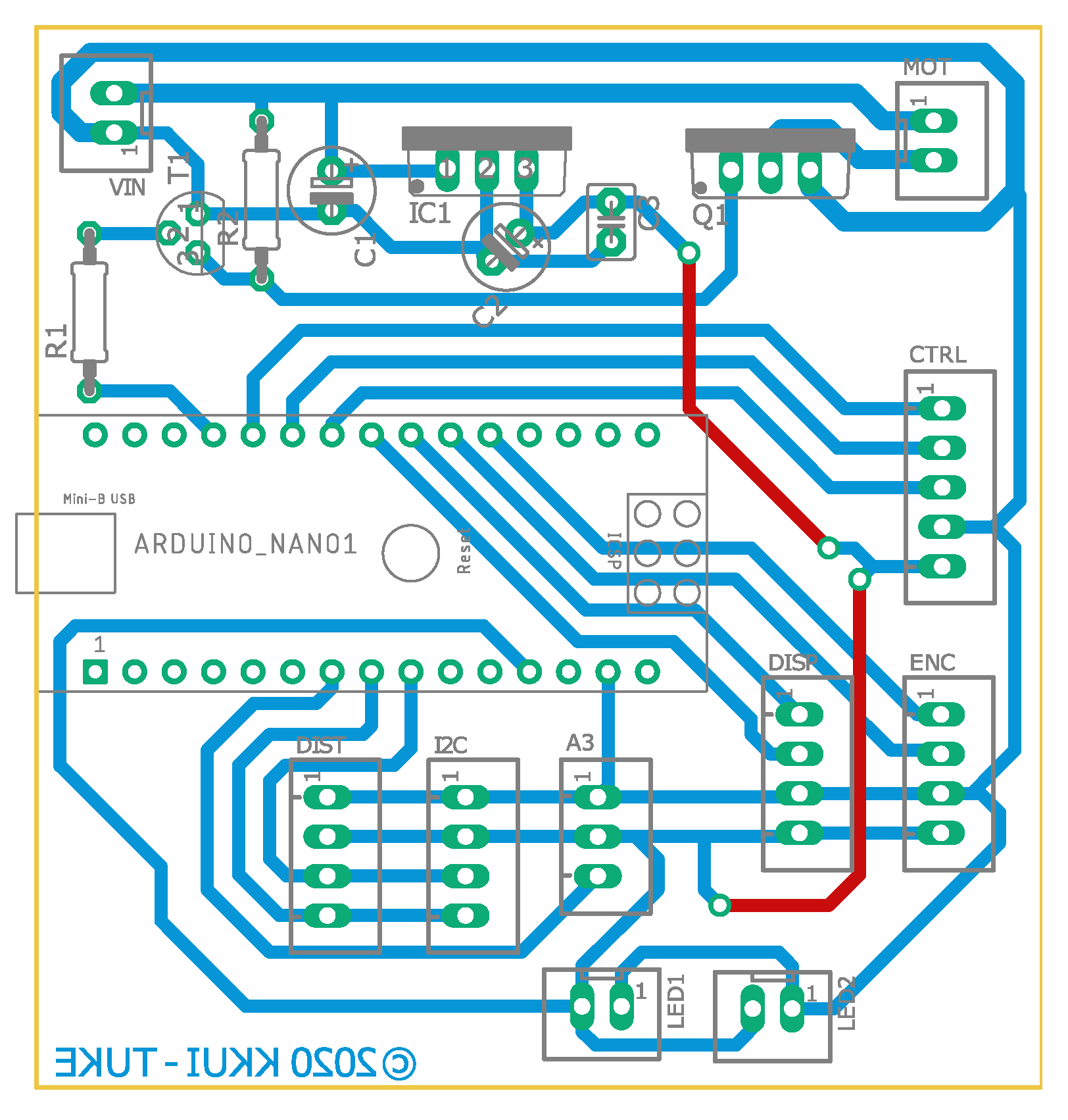
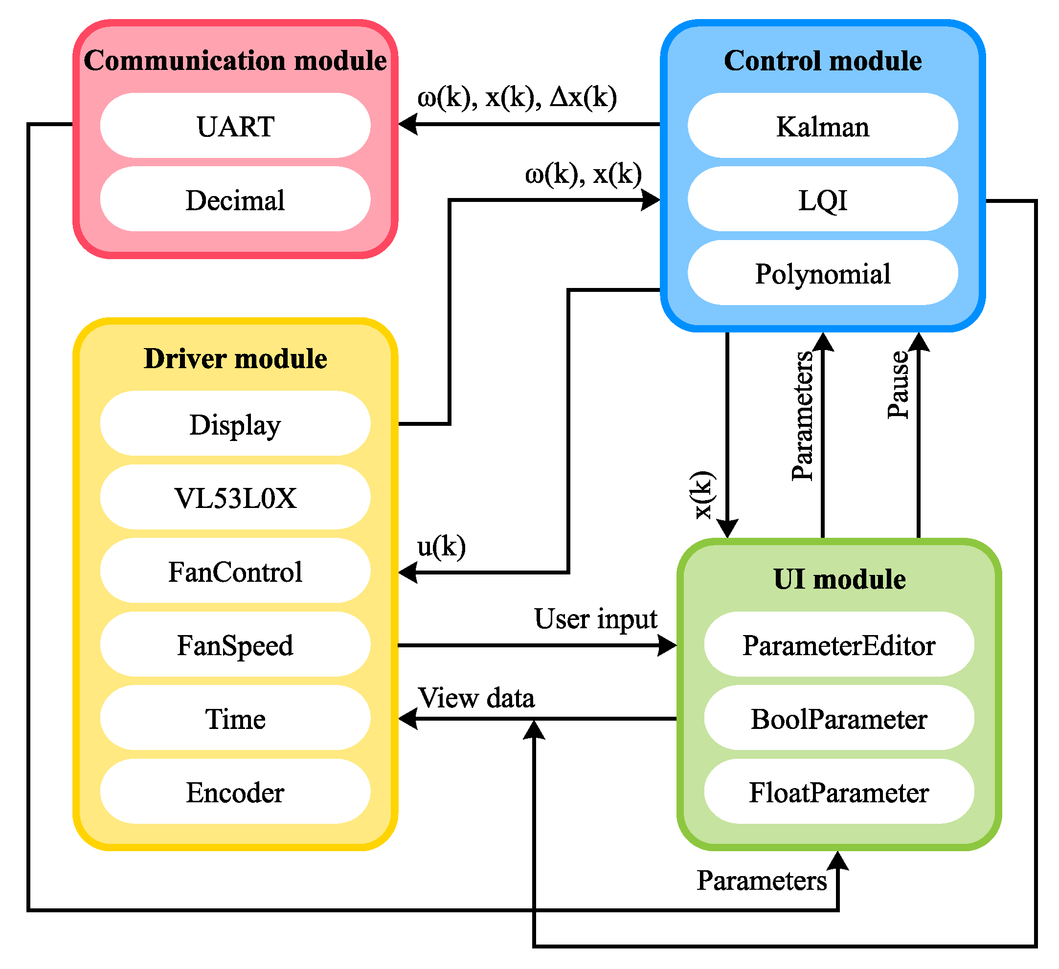
In this paper, we present the improved Aerodynamic Ball Levitation Plant with a fan speed sensor. We consider the addition of this sensor important for better plant control as it enables the use of more sophisticated control and state estimation algorithms. Furthermore, the additional sensor helps with the experimental estimation of the mathematical model’s parameters. The proposed methodology of the Aerodynamic Ball Levitation Plant modeling and control design is incorporated in the entire paper layout. This includes subtasks in the following order: mathematical modeling, creation of physical plant, experiment design, data acquisition, nonlinear parameter estimation, design of Kalman filter, controller design, validation in the simulation environment, and validation on the real plant. Methodology verification is presented in this paper using sets of experiment and their results.
The paper consists of several sections.
Section 2 deals with the construction of the Aerodynamic Ball Levitation Plant, whereas
Section 3 describes the analytical modeling and parameter identification of the mathematical model using the nonlinear least-squares method.
Section 4 deals with the design and validation of the Kalman filter and the optimal state-space controller with integrator (Linear-Quadratic-Integral control—LQI). Finally,
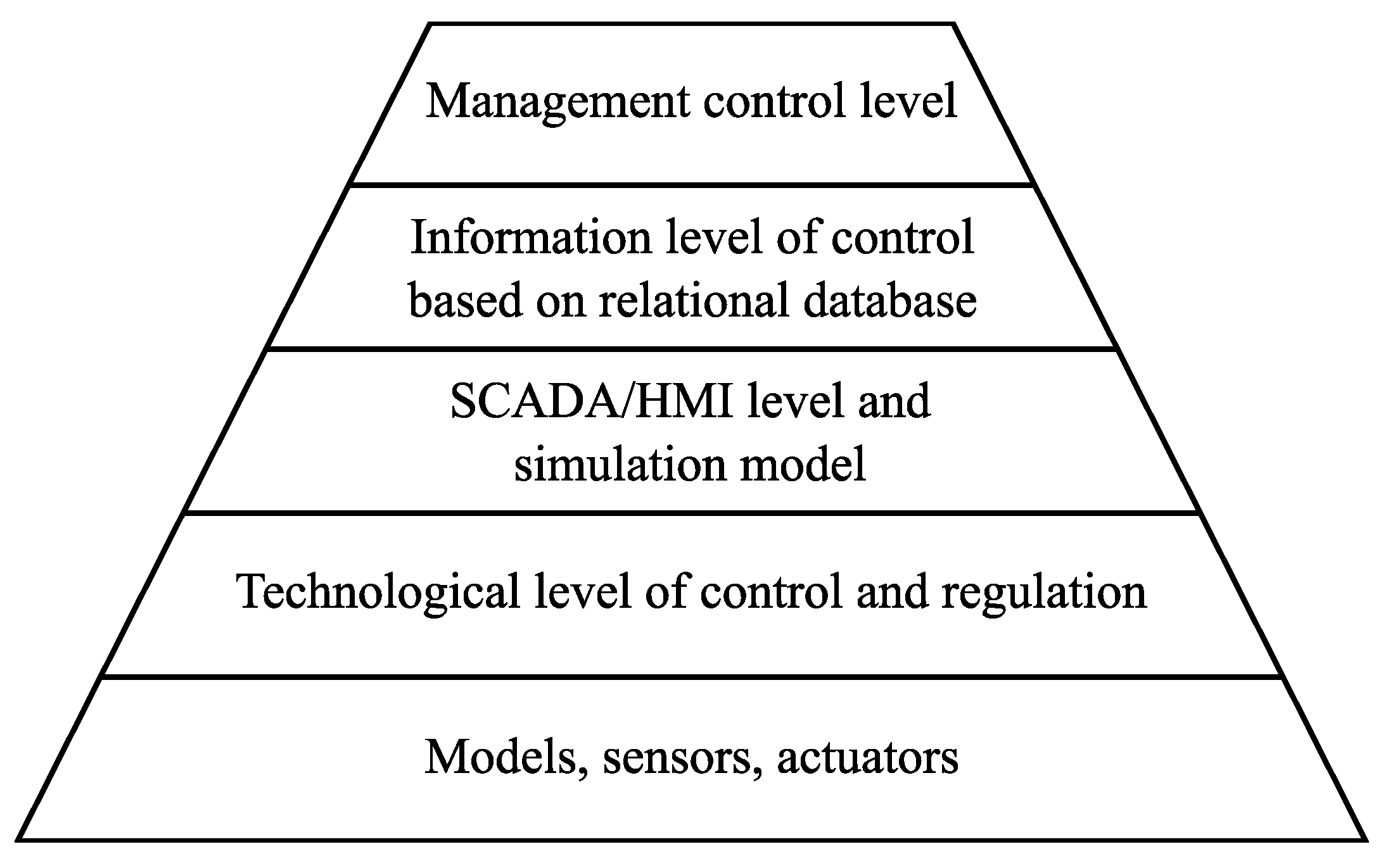
Section 5 describes the inclusion of the laboratory plant into the Distributed Control System (DCS) architecture at the CMCT&II.
3. Mathematical Modeling
In research papers [
4,
9,
16], a mathematical model of the Aerodynamic Ball Levitation Plant is presented as a single-input and single-output (SISO) system, with input being the fan’s voltage
and output the ball position
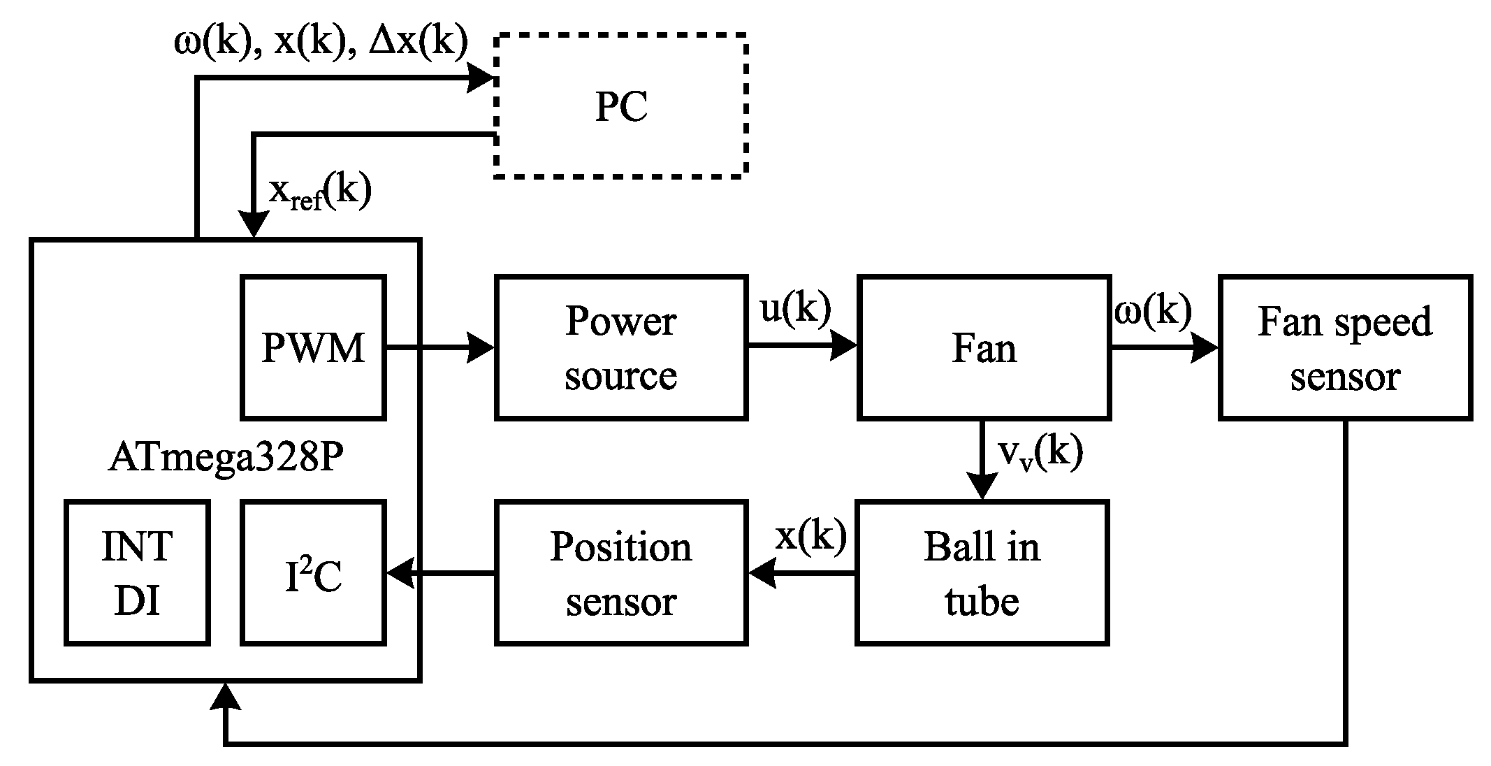
. Even though this representation does not affect the mathematical model itself, it is problematic during the experimental parameter estimation task. This is due to a high number of parameters and insufficient insight into internal system states. To overcome this limitation, our plant includes a fan speed sensor that enables us to model the system as a single-input and multiple-output (SIMO) system. To make the modeling task simpler, we are going to model two main subsystems (a fan and a ball in the tube) separately according to the diagram shown in
Figure 4.
Since our fan is driven by a DC motor, we can create its mathematical model using the kinematic equation for the rotational motion and Kirchhoff’s second law. Ignoring all nonlinearities, the resulting mathematical model is described by two first-order differential equations (Equation (
1)). State variables of this model are an armature current
and an angular velocity
[
18].
where:
J- rotor’s moment of inertia [kg.m
]
- rotor’s angular acceleration [rad.s]
- rotor’s friction constant [N.m.s]
- rotor’s angular velocity [rad.s]
- motor’s torque constant [N.m.A]
- armature current [A]
L- armature inductance [H]
R- armature resistance []
- motor’s back electromotive force constant [V.rad.s]
- motor’s input voltage [V]
To be able to use the proposed mathematical model (
1) of the fan for the parameter identification task, it is crucial to measure both of its state variables (
and
). Having sensors to measure both state variables (armature current
and rotor’s angular velocity
), it would be possible to use state-space control algorithms to control this subsystem. However, our hardware design does not include a current sensing circuit, so a slight model modification is needed. An approximation of the fan model in form of a linear first-order differential equation (Equation (
2)) was chosen for this task. Such a model has only one state variable (
) that can be measured with a rotary encoder included in our hardware design. Limitations of this approximation include slightly different system dynamics, the merger of system parameters, and the use of input–output based control algorithms. The parameter merging poses a problem if the physical interpretation of parameter value is required. This is not a problem as long as we intend to create a stabilizing controller.
where:
- fan’s damping factor [s
]
- motor constant [rad.s.V]
The ball in the tube subsystem shown in
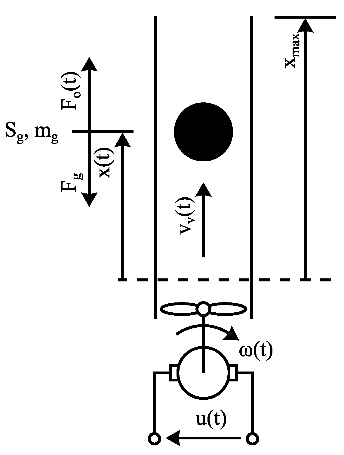
Figure 5 can be modeled using Newton’s second law if all forces acting on the ball are identified. To make it simpler, we consider only two major forces—a force of aerodynamic drag
and a gravitational force
that can be calculated using Formula (
3).
where:
- gravitational force [N]
- ball’s weight [kg]
g- gravitational acceleration [m.s]
Figure 5.
Simplified diagram of Aerodynamic ball levitation plant.
Figure 5.
Simplified diagram of Aerodynamic ball levitation plant.
The aerodynamic drag force depends on a ball’s drag coefficient
, ball’s cross section area
, density of the air
, and square of ball’s relative velocity as in (
4). The relative velocity is defined as a difference between air velocity
and ball’s velocity
.
where:
- aerodynamic drag force [N]
- ball’s drag coefficient [−]
- ball’s cross section area [m]
- air density [kg.m]
- air velocity [m.s]
- ball’s velocity [m.s]
Since air velocity
in the tube is relatively low, all mentioned factors except the relative velocity can be combined into a single constant
as in (
5).
where:
- ball’s drag factor [kg.m
]
According to the diagram in
Figure 5, both acting forces have opposing direction of the effect (
6).
where:
- force acting on the ball [N]
During normal operation, the aerodynamic drag force
is always acting in opposite direction to the gravitational force
. To make its direction of influence physically correct under all conditions, we added the sign function to the model Equation (
7).
where:
- ball’s linear acceleration [m.s
]
- sign function
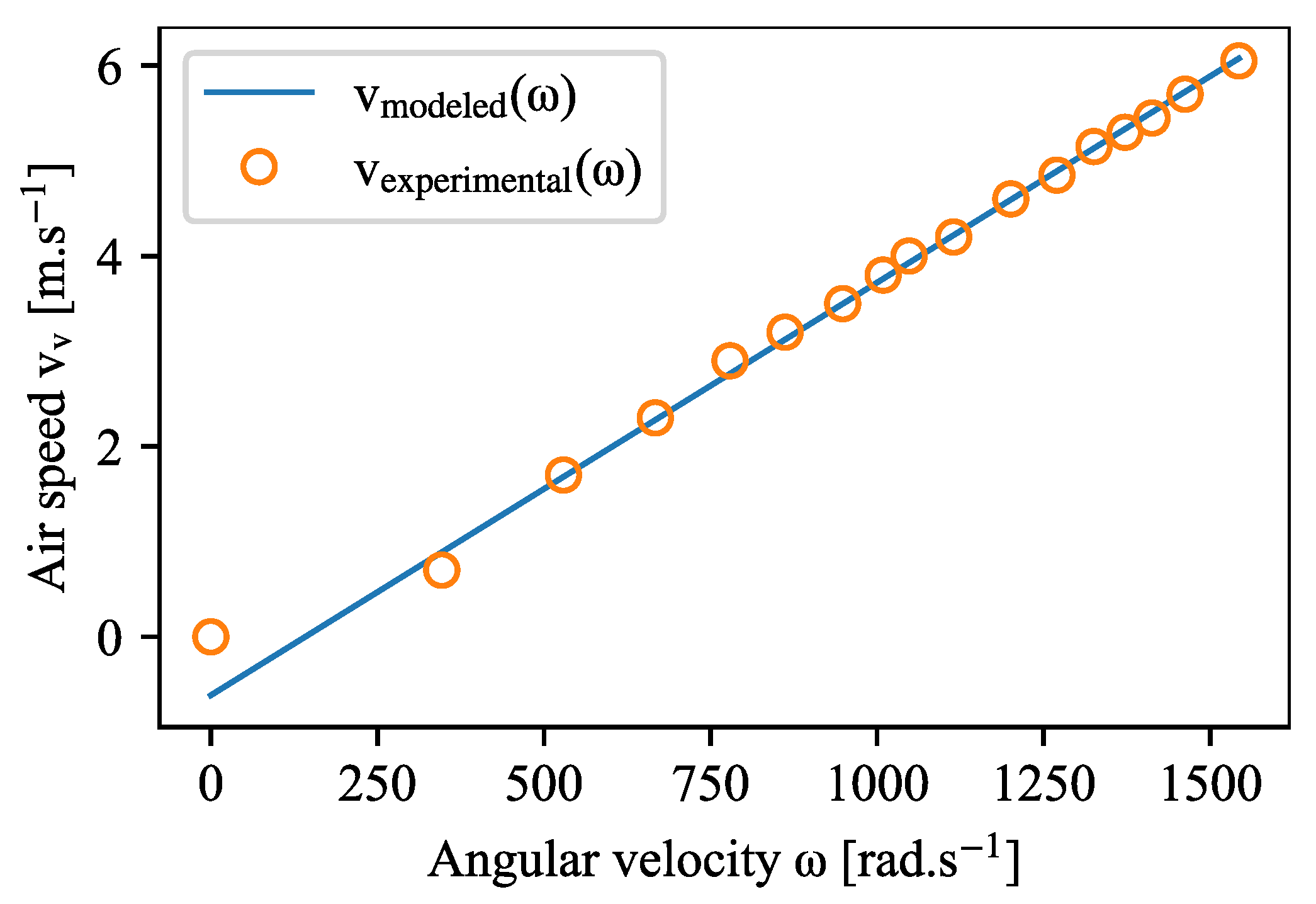
Finally, it is needed to find a link between the fan’s angular velocity
and air velocity
. According to our experiments shown in
Figure 6, the air velocity
has linear dependency on the fan’s angular velocity
as in (
8). A constant term is added to compensate for nonlinear behavior around zero.
where:
- fan’s coefficient [m.rad
]
- fan’s constant [m.s]
Figure 6.
Air velocity as a function of fan’s angular velocity .
Figure 6.
Air velocity as a function of fan’s angular velocity .
The complete mathematical model of the Aerodynamic Ball Levitation Plant is shown in (
9). Since this model contains several unknown parameters (
,
,
,
,
) that cannot be measured directly, we are going to estimate their values by means of experimental identification.
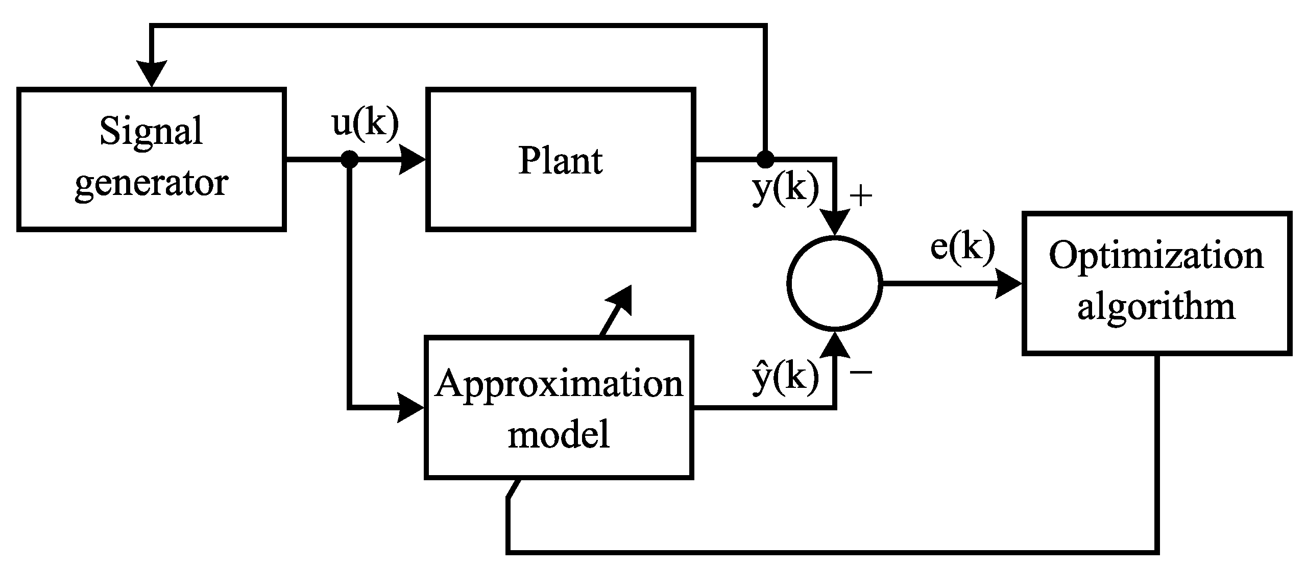
3.1. Experimental Identification and Model Validation
Experimental identification techniques can be divided by the type of resulting model into two major groups—grey-box and black-box model identification [
19]. As quite a few authors [
4,
5,
7,
16] have already put their effort into black-box model estimation [
20], we decided to focus on the first option and identify parameters of the plant model (
9) to create a grey-box model. The general schema of the identification topology is shown in
Figure 7, where in our case the approximation model is replaced with the analytical model (
9). Then an optimization algorithm is used to tune the model’s parameters to minimize the quadratic cost function (
10). This topology can be used for both online and offline identification tasks. Due to the fast dynamics of our plant, we opted for the offline variant.
where:
- quadratic cost function
- vector of model’s parameters
- output prediction error vector
- weighting matrix
Figure 7.
General schema for experimental parameter identification driven by output prediction error.
Figure 7.
General schema for experimental parameter identification driven by output prediction error.
Like the modeling, the parameter identification task can be also split into two parts according to the model subsystems. From the control engineering aspect, the fan subsystem is stable, and thus the identification can be performed in the open-loop using a pseudorandom rectangular input signal with varying amplitude. Because the ball’s presence affects airflow inside the tube, it was fixed inside the tube during the experiment. Obtained experimental data were used to estimate parameter values (
,
) of the fan’s model using
tfest function in MATLAB. The normalized root mean squared error of this model is 12.55% (the lower the better) and the adjusted R-squared value of this fit is 98.42%. Graphical model validation is shown in
Figure 8.
Parameter identification of the ball in the tube subsystem is a bit more challenging because this subsystem is inherently unstable [
5]. To overcome this issue, a closed-loop feedback controller must be used to avoid the ball’s position saturation at its physical limits. Instead of designing a full-fledged controller, we decided to go with a simple rule-based algorithm. This algorithm oscillates the ball around the center point by switching input value between
of equilibrium value. The time at which the input value is switched is always random to prevent harmonic oscillations. The parameters (
,
,
) of mathematical model (
9) are estimated by nonlinear least-squares method using a
nlgreyest function in MATLAB.
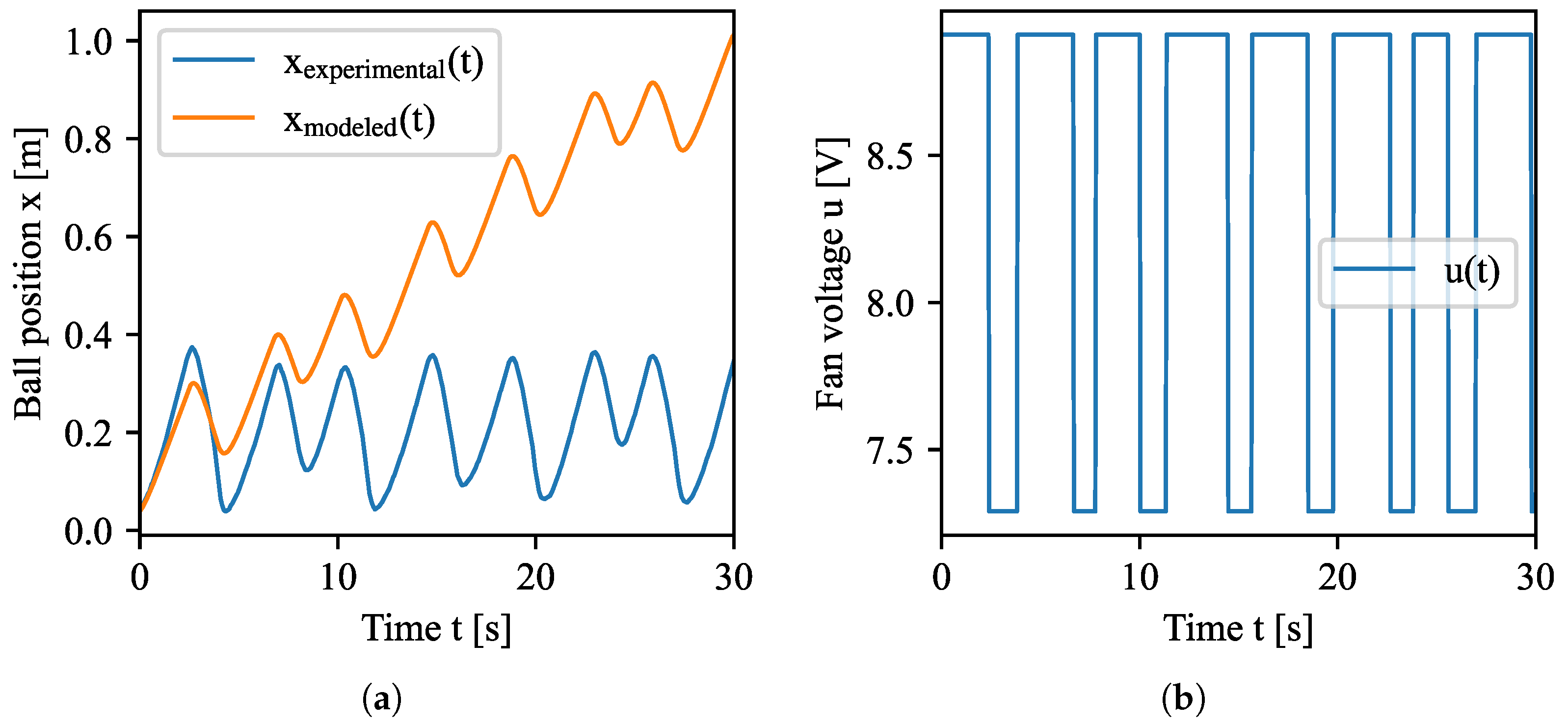
Results in
Figure 9 do not look promising at the first glance since the ball’s position of the identified model does not follow the position of the real ball precisely. This can be caused by a slight deviation in the value of some parameters and since the system behaves as an integrator, this error accumulates quickly over time. From the control engineering aspect, this should not be an issue in controller design as controllers must be robust enough to cope with system uncertainty. Values of estimated parameters are shown in
Table 1.
3.2. Linearization and Discretization
The mathematical model (
9) is not suitable for designing a discrete LQI controller, because this method is based on a linear discrete model in state-space form. To get the correct form, the model (
9) must be linearized first and then discretized. To make the notation of state vector cleaner, a substitution (
11) is proposed.
where:
- system’s state vector
= - fan’s angular velocity [rad.s]
= - ball’s position [m]
= - ball’s speed [m.s]
The mathematical model (
9) can be rewritten accordingly (
12).
In our case, the nonlinear model (
9) is linearized at a operating point selected in the center of the tube, while other values are calculated by substituting all derivatives (
9) with zero. Finally, the operating point can be defined by (
13).
where:
- linearization operating point vector
- operating point fan’s angular velocity [rad.s]
- operating point ball’s position [m]
- operating point ball’s linear velocity [m.s]
- operating point fan’s input voltage [V]
Linearization at the operating point
can be performed by expanding nonlinear model (
12) into first order approximation using Taylor series as shown in (
14), where
denotes output vector of a linear model [
21].
where:
Based on the sampling period
of the ball’s position sensor (
s), the linear model (
14) is discretized using the same sampling period value. The linear discrete model in state-space form is shown in (
15). This model is used to design an LQI controller.
where:
- discrete linear state matrix
- discrete linear input matrix
- discrete linear output matrix
4. Controller Design and Verification
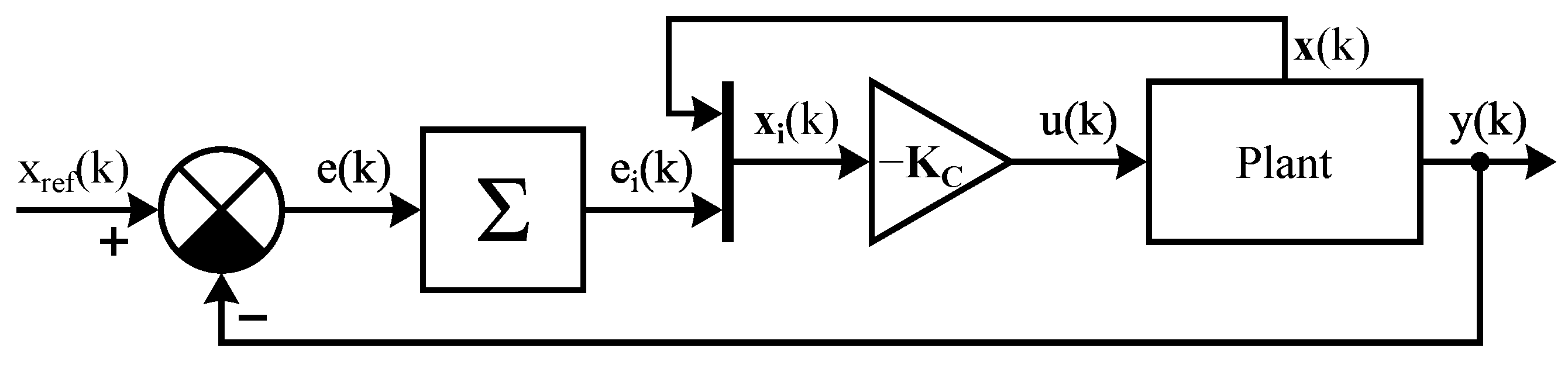
Thanks to the integrated fan speed sensor of our plant, a wide range of control algorithms can be utilized. Since plenty of previously mentioned authors have already worked on control algorithms based on the input-output model, the state-space control based on LQI has been selected.
Even with the addition of the fan speed sensor, it is not possible to measure the ball’s speed . To overcome this limitation, some kind of estimation is needed. The simplest solution is to estimate the ball’s speed using the difference of its position . Since data from the position sensor is quite noisy, the Kalman filter is used as both an estimator and a noise filter.
4.1. Noise Filtration
The Kalman filter uses a discrete linear model (
15) of the system with the addition of a system noise (
) and a sensory noise (
) (
16). System noise (
) is used as the result of ignored or approximated parts of the physical system’s dynamics, whereas sensory noise (
) is caused by the sensor itself or by the ADC conversion. It is expected that both system and sensory noise have a zero mean value and noise covariance matrices (
,
) are known. The extended Kalman filter is a modification that allows noise filtering of non-linear systems, as system matrices (
,
,
) are being updated in every step [
22]. From the perspective of the model (
12), it is sufficient to use the Kalman filter (not its non-linear variant) as the change in the ball’s position does not affect the linearized model, and the ball’s velocity is expected to have near-zero value.
where:
- discrete state matrix
- discrete input matrix
- discrete output matrix
Each iteration of the Kalman filter algorithm is divided into two phases—prediction and correction [
22]. During the prediction phase, a new system state is predicted using the system’s model, the previous state, and the value of the input (
17). The second phase uses measurements to correct the predicted states to get an estimate of the real system state (
18).
where:
- predicted value of the state vector
- corrected value of the state vector
- predicted value of error covariance matrix
- corrected value of error covariance matrix
- covariance matrix of the system noise
where: - Kalman gain matix
- covariance matrix of the measurement (sensory) noise
- measured system output
- identity matrix
The discrete linear model (
15) was used to design a Kalman filter. Noise covariance matrices (
,
) were fine-tuned using an experimental approach, so that measured noise is reduced while not affecting the dynamics of the physical plant. Exact values used are shown in (
19).
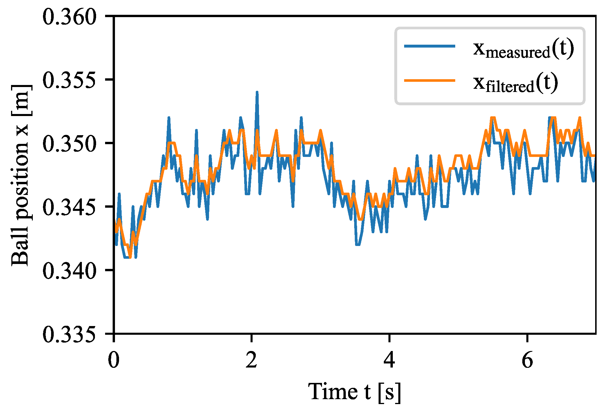
In
Figure 10, one can see the application of the Kalman filter in the task of noise filtration of the ball’s position
measurement. The visible noise reduction will have a positive effect on the control of the plant.
4.2. LQI Controller
The LQI controller is a variant of the standard Linear-Quadratic Regulator (LQR) that includes the integral term. The design of such controller starts with a discrete linear model (
15) of the plant. This model is firstly converted into its extended form (
20) that adds at least one state variable. How many state variables are added depends on how many state variables require zero error. Each added state variable resembles an integral of the error of the target state variable. This requires modification of the dynamics matrix
and input matrix
according to (
21).
where:
- discrete linear state matrix of model in extended form
- discrete linear input matrix of model in extended form
where: - sampling period [s]
The LQI controller is designed in the same way as the standard LQR controller [
23] by minimization of quadratic cost function (
22), which is modified according to the LQI needs.
where:
- quadratic cost function
- state weighting matrix
- input weighting matrix
and
weighting matrices are set according to (
23).
To get an optimal control algorithm based on cost function (
22), the Riccati algebraic Equation (
24) must be solved [
24].
where:
- solution of Riccati algebraic equation
Finally, controller (
25) in form of the feedback gain
can be calculated using the solution
of Equation (
24).
where:
- feedback gain
Before we apply the newly designed controller (
25) onto the real plant, its effectiveness needs to be verified in a simulation environment. For this task, a nonlinear mathematical model (
12) implemented in MATLAB/Simulink was used. The general schema for the verification of the LQI controller is shown in
Figure 11.
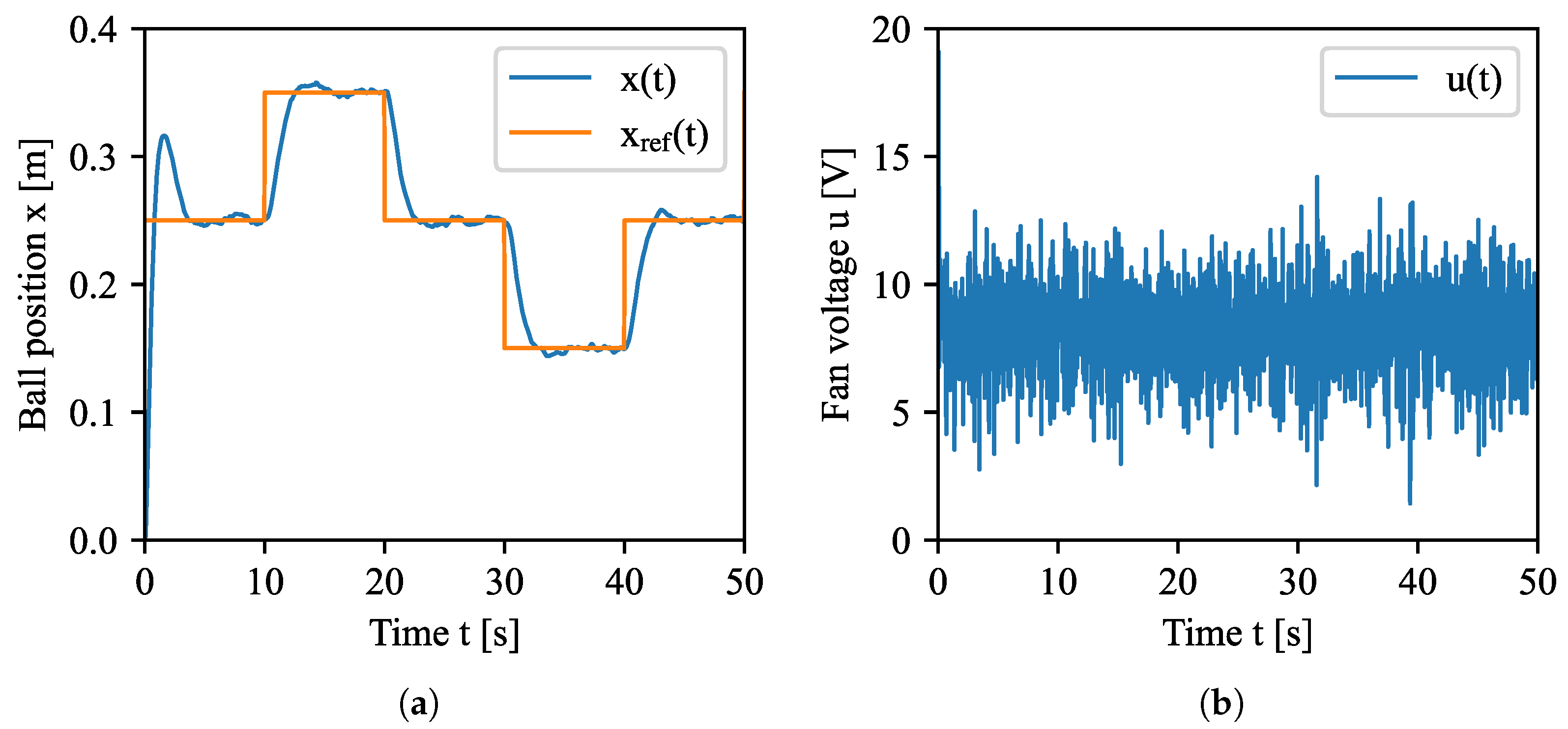
From the simulation results shown in
Figure 12, it can be concluded that the designed controller is sensitive to noise, but the regulation period is satisfactory. In this simulation, the Kalman filter was not applied while sensory noise was modeled as a standard Gaussian noise.
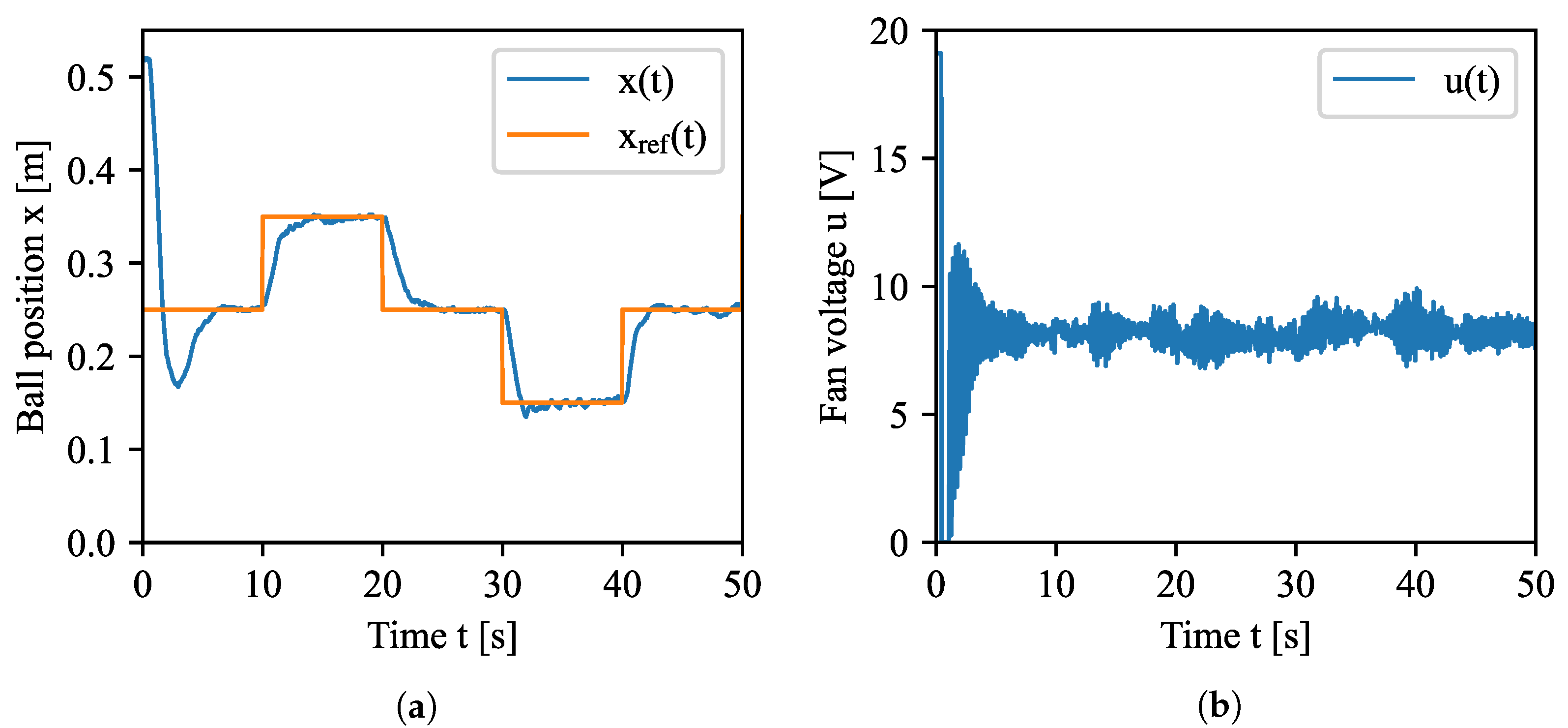
After successful simulation controller verification, the controller (
25) was applied on the real plant with results shown in
Figure 13. The deviation of the ball’s position
from a reference trajectory
near the zero time is caused by different initial conditions between simulation and real experiment. In the case of the real laboratory plant, the initial position of the ball must be at its topmost position within the tube. This prevents the ball from being stuck near the fan due to highly turbulent airflow at its close proximity.
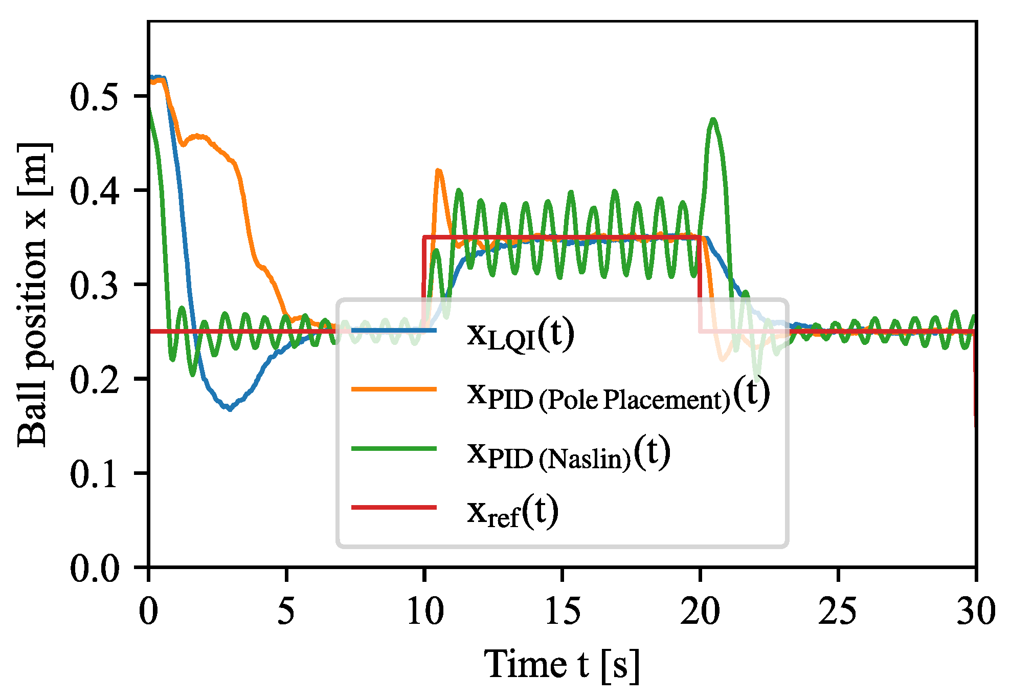
We also conducted position tracking experiments with a polynomial controller designed using the pole placement method and a discrete PID controller with trapezoidal integral approximation. Results shown in
Figure 14 depict a comparison of these control algorithms with the previously presented LQI control algorithm. The following parameters were used in the design of these controllers:
A quantitative comparison of the selected set of control algorithms is shown in
Table 2. Metric
quantifies how well the ball position
tracks the reference position
and its formula is in (
26). Metric
quantifies how stable is the fan’s voltage
and its formula is in (
27). The regulation time is the timespan it takes the ball position to reach
of reference the reference signal from the start of the experiment.
where:
- i-th sample of ball position
- i-th sample of ball reference position
where: - i-th sample of fan voltage
6. Conclusions
The main goal of this paper is to present obtained experimental results from the newly created Aerodynamic Ball Levitation plant. This includes the design and verification of a methodology for modeling, identification, control, simulation, and implementation on the real nonlinear laboratory plant. Additionally, details about hardware and software implementations are provided with the emphasis on design improvements. The main improvement of our design is the addition of the fan speed sensor that enabled us to use a broader range of available control algorithms. These control algorithms can be easily validated on the simulation model that acts as a digital twin for the real plant. The digital twin can be used for predictive control algorithms or to generate training data for AI-based controllers.
Another improvement was made in the use of the Kalman filter to filter the sensory noise, which in turn reduced the fluctuation of the control voltage. Lastly, the onboard control mechanism was added in form of the display and the rotary encoder with a push-button to control the plant without the need for a computer. Obtained results are presented in visual form supplemented with quantitative evaluation. The laboratory plant can be further improved, e.g., with the addition of a current sensing circuit. This circuit can improve the results of the experimental identification especially in the case of the fan subsystem. Additionally, a different set of control algorithms such as Model Predictive Control, Model Reference Adaptive Control, or Robust Tracking Control can be evaluated on this plant.
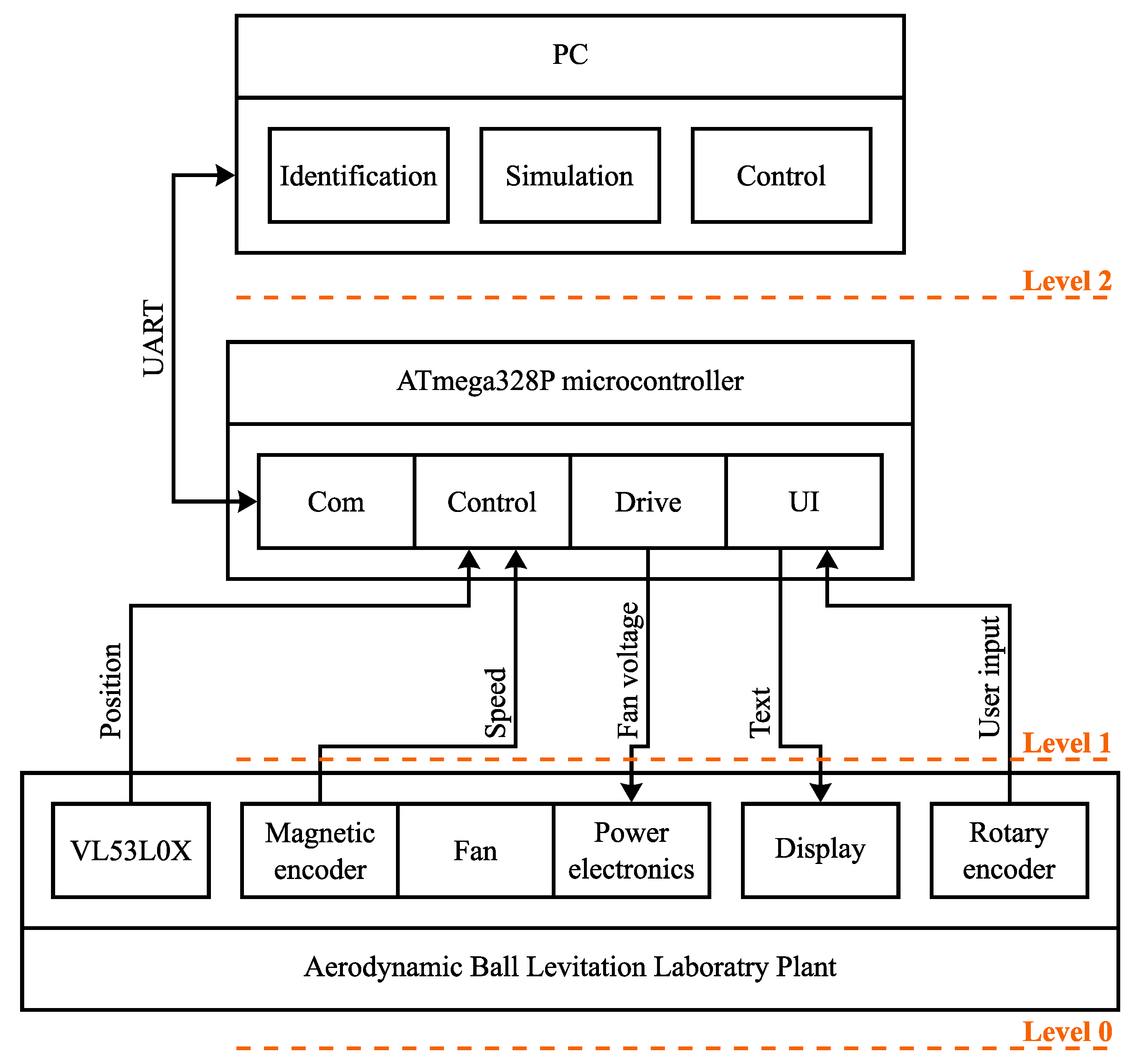
The newly created laboratory plant will be used in the education process during control engineering courses provided by CMCT&II, for example, Basics of Automatic Control, Optimal Control of Hybrid Systems, or Control and Artificial Intelligence. The plant creates a solid foundation for standard control engineering tasks, such as analytical modeling, parameter identification, and design of various types of controllers. It also enables the members of the CMCT&II to implement the laboratory plant into similar DCS architecture that is used at the CERN.


