Optimization of No-Wait Flowshop Scheduling Problem in Bakery Production with Modified PSO, NEH and SA

Abstract

In bakery production, to perform a processing task there might be multiple alternative machines that have the same functionalities. Finding an efficient production schedule is challenging due to the significant nondeterministic polynomial time (NP)-hardness of the problem when the number of products, processing tasks, and alternative machines are higher. In addition, many tasks are performed manually as small and medium-size bakeries are not fully automated. Therefore, along with machines, the integration of employees in production planning is essential. This paper presents a hybrid no-wait flowshop scheduling model (NWFSSM) comprising the constraints of common practice in bakeries. The schedule of an existing production line is simulated to examine the model and is optimized by performing particle swarm optimization (PSO), modified particle swarm optimization (MPSO), simulated annealing (SA), and Nawaz-Enscore-Ham (NEH) algorithms. The computational results reveal that the performance of PSO is significantly influenced by the weight distribution of exploration and exploitation in a run time. Due to the modification to the acceleration parameter, MPSO outperforms PSO, SA, and NEH in respect to effectively finding an optimized schedule. The best solution to the real case problem obtained by MPSO shows a reduction of the total idle time (TIDT) of the machines by 12% and makespan by 30%. The result of the optimized schedule indicates that for small- and medium-sized bakery industries, the application of the hybrid NWFSSM along with nature-inspired optimization algorithms can be a powerful tool to make the production system efficient.

1. Introduction

In an industrial production system, scheduling jobs is an important integral part. It refers to the arrangement of jobs to be processed on machines under some constraints. A production system can fail to be efficient due to the lack of planning and proper allocation of tasks among machines. In the literature, such problems are known as flowshop scheduling problems (FSSP) or a job shop scheduling problem and have been observed as NP (nondeterministic polynomial time)-complete combinatorial optimization problems when the number of machines exceeds two [1].

In FSSP, jobs are $n$ products, each of which consists of a set of tasks. These tasks need to be performed sequentially by a set of $m$ machines. In some flowshop environments, these tasks need to proceed continuously without any interruption in between, known as no-wait FSSP. In such cases, the production start time of a product can be independent. However, once it starts, the waiting time between two consecutive tasks is unacceptable. In a typical FSSP environment, all the products $\left(n\right)$ undergo all the machines ($m)$ in the same order, which is widely known as permutation FSSP.

In the bakery production system, the dynamic process involving physical and biochemical reactions, such as yeast fermentation, causes change in the behavior of the material. Due to the addition of living yeast cells, the dough is strictly sensitive to time and temperature as they affect CO₂ production significantly and thus influence the texture and aroma of the final product. Even though some processing steps, for example, dough rest and cooling after baking, may not require any energy-consuming machine, they have a certain duration for these tasks. Exceeding the predefined duration for a task causes overtreatment and delay for the next treatment. In a bakery production environment, both are unacceptable as they directly affect the product quality. Therefore, the processing tasks need to be performed accordingly in time. From this perspective, the bakery production schedule falls in the no-wait FSSP.

Abdollapour et al. presented a mathematical model of a flexible no-wait flow shop problem with a capacity restriction on the machines [2]. Bewoor et al. described a mathematical model of a no-wait flow shop scheduling model and proposed a hybrid particle swarm optimization algorithm to solve the scheduling problem [3]. Application of no-wait FSSP was provided by many other studies [4,5]. However, there are some exceptional characteristics in the bakery production system and very few authors have focused on this branch [6,7,8]. Therefore, there are opportunities to improve production modeling and optimization. Medium- and small-scale bakeries, even in many developed countries, are reportedly conducting production operations inefficiently [7], merely based on personal experience. A recent study reported that there are enough opportunities to improve production efficiency in the bakery industry by forecasting sales and optimizing the production schedule [9]. In this scheme, sales forecasting tackles the waste of food by predicting the market demand for each type of product and the optimized production schedule concerns minimizing the production cost of the predicted products in terms of time and energy consumption. However, this article focuses on the optimization of the production schedule and addresses a hybrid NWFSSM with an application in a bakery industry that involves several constraints and objectives that were not included in previous studies. By using the proposed model, a production schedule can be simulated and the cost of production, such as makespan, and the TIDT can be calculated. However, to find an optimized schedule with minimum cost, an optimizer must be integrated.

In the literature, many heuristic and meta-heuristic optimizations were proposed with their modification and showed a comparison of their performance by solving scheduling problems. In the early stage, the constructive approach, widely known as NEH [10], is probably the one mostly refined and modified by other authors [11]. On the other hand, many meta-heuristics and their modified approaches have been applied to solve FSSP, such as particle swarm optimization [12,13], simulated annealing [14], genetic algorithm [13,15,16], ant colony optimization [7], and firefly algorithm [17].

Ever since the PSO algorithm was introduced by Eberhart and Kennedy [18], it was demonstrated that despite being a powerful algorithm, it easily falls into a local minima when solving complex and high dimensional problems [19]. Moreover, a common disadvantage of nature-inspired evolutionary optimization algorithms, like PSO, is that there is no certainty of always achieving a better result. Studies have found that a simple change in the PSO algorithm reportedly increases the performance effectiveness in terms of finding a quality solution to FSSP within a reasonable time. By adjusting the random value in the acceleration of a particle using a prescribed probability, PSO reportedly can avoid being trapped in local minima [20]. The addition of local search functionality in the PSO algorithm was presented to have improved performance [21,22]. A robust hybrid PSO algorithm was proposed by Ji et al. [23] where PSO-Based exploration and SA-based exploitation were integrated. Similarly, Issa et al. proposed a scheme of merging PSO with a recently proposed sine cosine optimization algorithm to impose optimum exploration and exploitation in searching the solution [24].

In this research, we propose a modified PSO (MSPO) to tackle the issues associated with providing premature optimization results by implementing the subtraction operator. The behavior of PSO concerning exploration and exploitation due to the change in acceleration parameters was investigated to solve the “no-wait” flowshop scheduling problem effectively. An existing production line of a bakery was taken as a case with the objectives of minimizing the makespan and TIDT. The performance of MPSO was compared with standard PSO with two different configurations (PSO-A, PSO-B), SA, and NEH. The robustness and frequency to surpass a certain level of optimization result were investigated. The main contribution of the paper can be summarized as follows:

• Develop an application of the optimization algorithms to improve the efficiency of the existing bakery production line by delivering a realistic schedule with reduced makespan and machine idle time.
• Thoroughly present the formulation of a hybrid “no-wait” flowshop model (NWFSSM) in the bakery industry where a product follows a set of sequential tasks. However, the order, duration, and required machine for the tasks might be different for different products.
• Carry out modification to standard PSO to avoid premature convergence to the local optimum solution.
• The proposed strategy requires no significant additional computational time, and implementation is as simple as standard PSO yet highly effective.
• Demonstrate a performance comparison between MPSO and standard PSO, SA, and NEH to give an impression of how reliable the proposed method is.

The rest of the paper is organized as follows. Section 2 describes the formulation of the bakery scheduling problem and modifications in the PSO algorithm. Section 3 shows the comparative performance analysis of modified and standard PSO, SA, and NEH in solving the bakery scheduling problems.

2. Materials and Methods

The formulation of the bakery scheduling problem, simulation, and all optimization algorithms were performed on a computer running Windows 10 as the operating system with a configuration of an Intel Core i5 at 4 × 3.20 GHz, 8.00 GB ram. The simulation of the hybrid NWFSSM and optimization algorithms were programmed and performed using the programming language Python 3.7 [25].

In this study, two problem sets of bakery production data were used, which were collected from two European small- and medium-sized enterprise bakeries. In problem I, the bakery had 21 different product batches and was used to simulate the current production schedule. In the next step, the optimization algorithms were performed to find an optimized schedule and compared with current production efficiency.

The second case, problem II was taken from Hecker et al. [6] which had 40 product batches. The authors described a no-wait flowshop model for that bakery production and performed standard PSO to optimize it. Therefore, problem II was chosen to compare the performance of the proposed MPSO with that study.

2.1. Bakery Production System

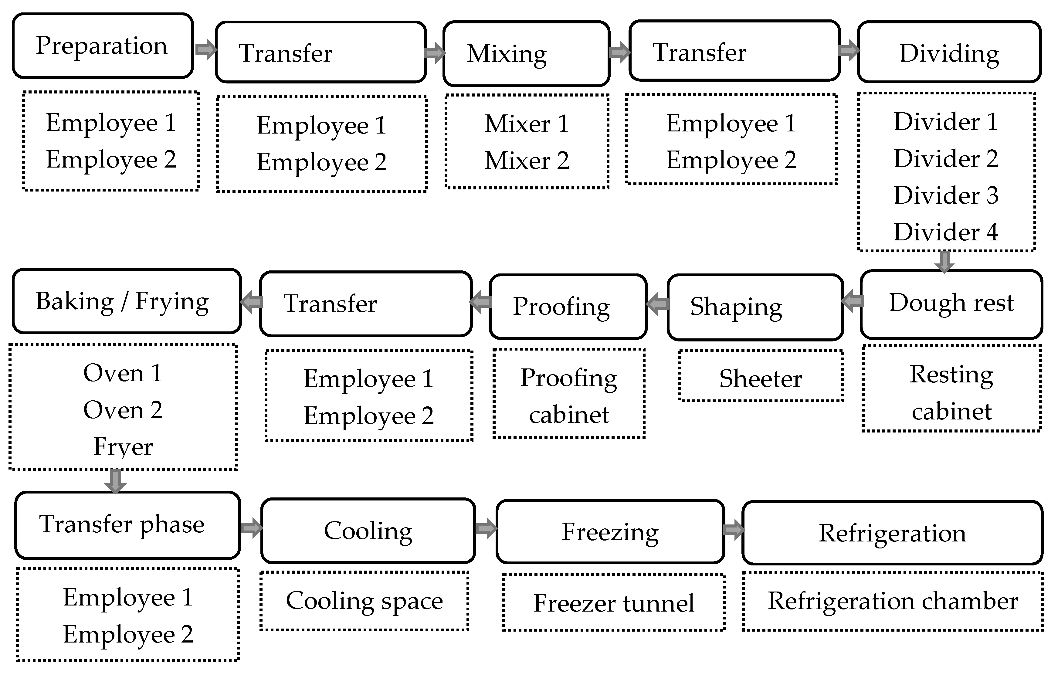
Each product in the bakery has a recipe, from a scheduling perspective, which is the combination of the number of processing tasks and the sequence of these tasks. Figure 1 shows a typical production line in a bakery. However, the recipes can vary in many aspects, such as the total number and sequence of the tasks, use of a specific machine, machine set up (e.g., temperature), and duration for the tasks. Furthermore, many tasks are performed manually e.g., loading flour, yeast, salt, and water into a mixer, transferring dough into a fermentation chamber, or baking oven. This considers that only machines and machine capacity in scheduling may overlook the limitation of the manpower. Additionally, to conduct one task, there are multiple alternative machines in bakeries. The number of alternative machines for different tasks is also different (Figure 1). As a result, the task allocation procedure in bakery production is different than most of the production systems. Therefore, a real bakery production scheduling problem can not be considered as permutation FSSP, rather such a model can be categorized as a hybrid-NWFSSM [26].

2.2. Problem Description

The problem dealt with in this paper can be discussed in two parts. Firstly, a hybrid NWFSSM was required to simulate the bakery production schedule. The main difficulty here was to integrate a set of constraints to reflect the actual production. It was expected that hybrid NWFSSM provides some information to evaluate one simulated production schedule. In bakery production efficiency, the main focus lies on the makespan and TIDT of the machines as they consume energy. Therefore, the output of the hybrid NWFSSM was the makespan and TIDT calculated from the simulated production schedule.

Secondly, an optimized schedule had to be found that has a minimum makespan and TIDT. The possible ways to schedule the production of $n$ products can be found from a permutation of $n$ items without repetition but in a different order of items. Mathematically, it can be expressed by $P\left(n\right)=n!$. In other words, the only difference between $n!$ schedules is the order of $n$ products i.e., which product should be produced when. However, this can influence production efficiency significantly. If the order of $n$ products in which they will be produced is changed, makespan and TIDT will also be changed. Moreover, if $n$ is higher, the possible ways to schedule are also increased by $n!$. For 21 product batches in problem I, there are 5.1 × 10¹⁹ possible production schedules. The main difficulty is that there is no exact method to find the best schedule in a shorter period of time. Using mathematical programming, all possible solutions can be calculated and evaluated to find the optimal schedule. However, it might take a long computation time. Therefore, many heuristic and metaheuristic optimization algorithms have been used to solve such problems. In such cases, the optimization algorithms may not find the best possible solution, but an almost best solution, which is usually better compared to what actually followed by the bakeries.

In this study, PSO, MPSO, SA, and NEH were performed to search for an optimized schedule from the massive number of options.

2.3. Objective Function

In this study, the main objectives were to reduce the makespan and TIDT of the machines in bakery production. It can be described as follows:

$$Cost=C_{max}+WTIDT$$

(1)

where $Cost$ is the cost of optimized schedule, $C_{max}$ is the makespan, and $WTIDT$ is the weighted total idle time of the machines. In the objective function, $C_{max}$ is the exact makespan of an optimized schedule and WTIDT is calculated from the idle time of the machines of the same schedule using weighting factors (explained in Section 2.4). The weighting factor for a machine should reflect the cost due to the energy consumption contributed in total production cost. The highly energy-consuming machines should have a high weighting factor, hence a smaller increase in idle time would have a bigger impact on the total cost compared to the other machines. In this study, the weighting factor for the machines were chosen, such that WTIDT for the existing schedule was lower than the makespan. However, it completely depends on the goal. If any bakery wants to focus more on the idle time reduction of the machines, the weighting factors for individual machines can be tuned such that WTIDT is bigger than the existing schedule’s makespan. The cost reduction due to the optimization algorithm was calculated using Equation (2).

$$Cost \mathrm{reduction}=\frac{Cos{t}_{opt}}{Cos{t}_0}\times 100$$

(2)

where $Cos{t}_{opt}$ and $Cos{t}_0$ are the cost from optimized and existing production schedules, respectively calculated using Equation (1).

2.4. Hybrid NWFSSM for the Bakery Production

The ‘no-wait’ flowshop scheduling model for bakery production proposed by Hecker et al. [6] was implemented to simulate new production data. However, since the proposed model was strictly for one bakery, some limitations had to be overcome to make a new model to reflect real production scenarios, which will be discussed in this section.

Table 1. Example production data for three products.

Product Name	Processing Stage	Duration	Resources
Sourdough	1. Preparation	3	Employee
	2. Mixing	13	Mixer
	3. Transfer phase	1	Employee
	4. Proofing	360	Proofing cabinet
Square bread	1. Preparation	3	Employee
	2. Mixing	16	Mixer
	3. Transfer phase	1	Employee
	4. Dough rest	15	Resting cabinet
	5. Dividing	3	Divider
	6. Molding	10	Employee
	7. Proofing	75	Proofing cabinet
	5. Baking	18	Oven
	6. Cooling	360	Cooling cabinet
	7. Freezing	70	Freezer
	8. Packaging	10	Employee
Pan bread	1. Preparation	3	Employee
	2. Mixing	12	Mixer
	3. Transfer phase	1	Employee
	4. Dividing	4	Divider
	5. Shaping	5	Shaper
	6. Proofing	85	Proofing cabinet
	7. Baking	14	Oven
	9. Cooling	60	Cooling cabinet
	10.  Freezing	70	Freezer
	11.  Packaging	10	Employee

shows an example of production data. It shows that the number and order of processing stages are different for the products that are in the common practice of the bakery industry. In this example, square bread has dough rest as a processing task, while pan bread requires no dough rest. Moreover, the number of stages for sourdough, square bread, and pan bread are 4, 8, and 11, respectively. The number and order of the stages may vary depending on the recipe of the products, which also varies from bakery to bakery. Therefore, it is difficult to make a common order of processing stages with a higher number of products that will work for every bakery industry. Moreover, the addition of a new product may require modifying the order of processing stages.

In their study, Hecker et al. [6] proposed an idea to make an order by mixing machines and processing stages. In the proposed order, 26 stages were shown despite the maximum stage for any product being 12. The idea was to make a common route for all the products. If a certain stage or machine in the route is not relevant to a product, it can be ignored by setting a 0 min processing duration. The machine for a task was kept fixed, although it is more flexible in practice. For instance, baking a product can be done either in Oven 1 or Oven 2 as there are mostly multiple alternatives for the same processing task. Moreover, in the bakery, many processing tasks are conducted manually by employees. It is practical to consider the limited capacity of the employees, which was ignored in the model proposed by Hecker et al. [6]. Moreover, the evaluation criteria of a schedule, either makespan or TIDT was used by the authors.

To eliminate these limitations in previous studies, a new flowshop model was created, the main features and constraints of which can be explained as follow.

▪

The name, number, and order of the stages for the products are independent. We propose no common route, rather it will be according to the original recipe. Therefore, due to the addition or deletion of a product, the complexity regarding the order of processing tasks can be ignored.

▪

Instead of fixing the machines, alternatives for a task are proposed. As a result, during task allocation, the algorithm will try to allocate the task for all products among these alternatives in a way that the overall makespan and WTIDT will be the lowest for a production sequence.

▪

The shift plan of employees is integrated, thus tasks are allocated within their working plan. Moreover, the conflict in manual tasks is avoided. Since delay between tasks is unacceptable, and interruption in one stage may cause delay to other stages and products, the task allocation for employees was found to be vital.

▪

The addition of new products and machines may require searching for a new optimized schedule as workload and capacity, respectively rise. Change in the shift plan or number of employees can also influence the overall production efficiency. Similarly, a machine, for instance, an oven can be added in the machine alternatives for baking to observe its influence on the production efficiency. The proposed model allows simulating the production by adapting such changes and monitor the efficiency to help the administration in decision making.

▪

Instead of a single objective, both makespan and WTIDT were taken into consideration to find a cost-effective solution to the production schedule. The WTIDT reflects the contribution of each machine in the final production cost.

Figure 2 illustrates the procedure of solving a given bakery production scheduling problem. The working principle can be described in four sections, namely, production data, hybrid NWFSSM, optimization algorithms, and visualization of results. In the production data, the name of the products, processing stages, start time, finish time, used machine for each stage, shift plan for employees, and current production sequence were recorded. The extracted information was used to simulate the schedule using hybrid NWFSSM. The output of the model is makespan and WTIDT for any production sequence. Afterward, the optimization algorithm executes and searches for an improved solution set, which is delivered back to the hybrid NWFSSM. The updated solution is converted into a sequence of production to make a new schedule and evaluation. This procedure is repeated until a certain termination criterion for one run is met. At the final stage, the schedule is visualized and cost reduction in terms of makespan and WTIDT is presented.

The progress of hybrid NWFSSM is presented in Figure 3. The assumptions and constraints are as following:

▪

Let us assume a production line has $n$ products P $\in \{P_i |i=1, 2, 3,\dots ,n\}$, where P indicates the set of products.

▪

To complete the processing of these products, there are $m$ machines M $\in \{M_k |k=1, 2, 3,\dots ,m\}$ and e employees E $\in \{E_l |l=1, 2, 3,\dots ,e\}$.

▪

$P_{i,s}$ refers to one processing time of product $P_i$ at stage s where $s=\left\{1, 2, 3, \dots , S_i\right\}$ and $S_i$ is the final stage for the product $P_i$.

▪

A set of alternatives, either machines or employees that can perform $P_{i,s}$ processing task is $A_{i,s}$ where $A_{i,s}\subset M$ or $A_{i,s}\subset E$.

▪

None of the machines and employees can process more than one task at a time.

▪

It is assumed that machines are available from the beginning to the end of the production time.

▪

The task allocation among employees must follow their working schedule such that none of the allocated tasks is scheduled out of their availability.

The allocation of tasks among machines and employees was performed by using Algorithm 1. The makespan $(C_{max})$ and weighted total idle time (WTIDT) of machines were calculated by Equations (3) and (4) respectively.

$$C_{max}=maximum\left(\left\{f_i | i=1, 2,\dots ,n\right\}\right)$$

(3)

where $f_i$ is the finish time of the product $P_i$.

$$WTIDT={\displaystyle \sum _{k=1}^m}\left(en{d}_k-star{t}_k-{\displaystyle \sum _{i=1}^n}p{t}_{i,k}\right)\times W_k$$

(4)

where $k$ denotes one machine from a total number of $m$ machines, $star{t}_k$ and $en{d}_k$ refer to the production time when machine $k$ started and ended respectively, $p{t}_{i,k}$ is the processing time of the product $P_i$ that was allocated to the machine $k$ and $W_k$ refers weighting factor for idle time of machine $k$.

In a bakery production environment, the idle time of all the machines is not equally important for the cost of production. These machines can be used immediately after switching on, and hence no energy is consumed during idle time. In contrast, several machines e.g., ovens require to run a certain time to fulfill the settings required to perform the processing task. In such cases, to avoid the unexpected interruption in the production, the machines are mostly kept running even when no products are processed. The idle time of these machines must be pronounced with a higher weighting factor as it increases the overall production cost. Therefore, $W_k$ was used to discriminate the machines in contributing to the cost function through WTIDT in Equation (1). WTIDT was used only for optimization purposes to represent the cost due to the TIDT. In contrast, TIDT refers to the sum of the idle time of all the machines in a schedule. TIDT was calculated by using Equation (4), just as with the WTIDT, however with $W_k=1$ for all the machines.

Algorithm 1. Tasks allocation procedure.
1	begin
2		generate a solution // e.g., from PSO
3		sort jobs $\left(J\right)$ according to the given solution // e.g., SPV rule
4		for$P_i$ = 1 to n do // for all the products
5			for$sm=t_0$totfdo // start minutes for $P_i$ e.g., $t_0, t_1, \dots , t_f$
6 7				$s=1$, $s{t}_s=sm$ // start time for first stage uninterrupted = True // no-wait constraint
8				whileuninterrupted is True and $s\le S_i$ // for all the stages
9					$task minute{s}_{i,s}=\left\{s{t}_s, s{t}_s+1,\dots ,s{t}_s+p{t}_{i,s}\right\}$
10					resource available = $False, alternative$ = 1
11					whileresource available is False and $alternative\le A_{i,s}$
12						if$alternative$ is free during $task minute{s}_{i,s}$
13 14 15							Allocate task to this alternative resource resource available = True // break loop (line 11) $s=s+1$, $s{t}_s=s{t}_s+p{t}_{i,s}$ // start time for next stage
16						else try with next alternative
17							$alternative=alternative+1$
18					ifresource available = False // no alternative is free
19 20							uninterrupted = False // no-wait constraint is interrupted // break loop (line 8) and try with a new $sm$ (line 5)

To illustrate the proposed NWFSSM, there are 3! = 6 possible production sequences to produce three products e.g., sourdough, square bread, and pan bread (Table 1). For simplicity, no alternative machines are shown. Proofing, dough rest, cooling cabinets, and freezer are considered to have the capacity to operate three products at a time. The rest of the resources can operate only one product at a time. For instance, if the mixer is occupied for square bread, the mixing of pan bread cannot be executed during this time as there is only one mixer and it can operate one product at a time. If a production sequence of {sourdough, square bread, pan bread} is followed, the schedule is presented in Figure 4.

According to the schedule, the makespan is 289 min as this is the maximum time any product is finished. The idle time for the oven is 2 min. However, if the production sequence is changed to {pan bread, sourdough, square bread}, the values are changed to 295 min, and 7 min respectively.

2.5. Optimization Algorithms

2.5.1. Modification to Standard PSO

PSO is a metaheuristic optimization algorithm inspired by the behavior of animals like birds on the food search. The position of one particle or individual carries one solution to the given problem. The particles search the solution in a space in the form of multi-paths obliged by the movement in a swarm following a quasi-likelihood function. The instant movement and direction to which a particle moves are controlled by two dominant positions in the space i.e., current global best position and best personal position. The former offers the best solution to the problem and the latter is best in the solution history of the corresponding individual particle.

Each movement results in a change of the position of the particle, thus a new solution is proposed. The motion of particles is controlled by velocity parameters. In standard PSO, the velocity control parameters are proposed to be constant over the runtime. However, in this study, a certain modification to accelerate the movement of particles is proposed which consequently would come across with a complementary solution from the updated particle position. The integration of parameters $\alpha$ allows PSO to revise the motion of the particles shown in Equations (5)–(7).

$$v_i^{t+1}=v_i^t\times W+C_1^{t+1}\times r_1\odot \left[g^{*}-x_i^t\right]+C_2^{t+1}\times r_2\odot \left[x_i^{*}-x_i^t\right]$$

(5)

$$x_i^{t+1}=x_i^t+v_i^{t+1}$$

(6)

$$C_1^{t+1}=C_1^t+\alpha$$

(7)

where $C_1^{t+1}$ and $C_2^{t+1}$ indicate the velocity parameters, $v_i^{t+1}$ is the velocity, $x_i^{t+1}$ is the updated position vector of particle $i$ at iteration $t+1$, $g^{*}$ is the global best position, $x_i^{*}$ is the personal best position in the history of particle $i$, $W$ is a parameter that controls the influence of the previous velocity of the particle, $r_1$, $r_2$ refer to the random numbers between 0 and 1, $\odot$ indicates the multiplication of a scalar with a vector, and $\alpha$ is the acceleration parameter.

Equation (6) is the addition of three velocities, where the first part refers to the velocity in the previous movement $\left(t\right)$, like inertia, the second part is called social velocity, and the third part is cognitive velocity. In standard PSO, parameters, $W$, $C_1, \mathrm{and} C_2$ are kept constant over a runtime, which means a constant influence of three velocities on the final movement. In this study, Equation (5) was added to modify the parameter $C_1$. A negative $\alpha$ indicates a decrease of $C_1$ with iterations, and vice-versa. Therefore, the ratio of $C_1 \mathrm{and} C_2$ is changed over a runtime, and thus the relative influence of social and cognitive velocity in the final movement.

Table 2. Configuration of acceleration parameters in particle swarm optimization (PSO) and modified PSO (MPSO) for 50 iterations.

Configuration	Version	$\mathit{W}$	${\mathit{C}}_1$			${\mathit{C}}_2$
			Iteration = 0	$\mathbf{\alpha }$	Iteration = 50
PSO	PSO-A	0.50	1.00	-	1.00	1.80
	PSO-B	0.50	1.00	-	1.00	1.00
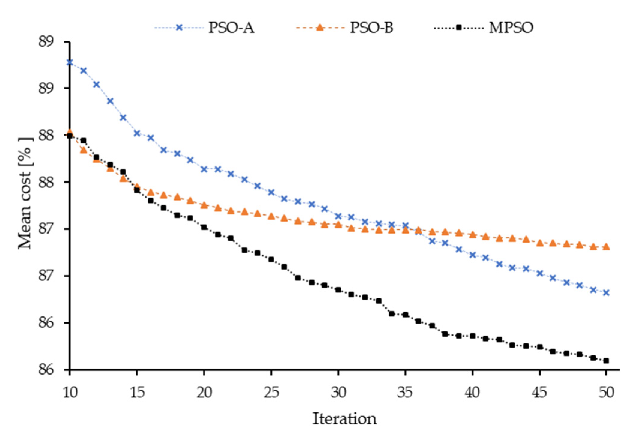
Modified PSO	MPSO	0.50	1.80	−0.02	0.80	1.00

shows the values of acceleration parameters for standard PSO (PSO-A, PSO-B) and modified PSO (MPSO). The value of $\alpha$ depends on the number of iterations, and the initial value of $C_1 \mathrm{and} C_2$, which can be described by the following equation.

$$\alpha =\frac{C_2-C_1}{d\times total iteration}$$

(8)

where C₁ and C₂ are velocity parameters and C₁ > C₂, d determines how many iterations the value of C₁ would be higher than C₂. For this study, d was set to 0.80 which indicates that from the beginning to 80% of total iterations, the value of C₁ was higher than C₂.

Figure 5 shows the change in the ratio of $C_1 \mathrm{and} C_2$ over a runtime. It explains how the ration of social and cognitive velocity is also indirectly controlled where the social velocity is more prominent at the initial phase and cognitive velocity is given more strength at the later phase. Therefore, particles in MPSO tends to move to the individual best position at the later phase which may lead to a new global best position instead of being stuck in the current best position. For a new optimization problem, the global optimum is unknown, hence, metaheuristic algorithms like PSO cannot differentiate local optima from global optimum. Since PSO is based on the food-searching behavior of animals, it never stops in one location. The efficiency of searching for an improved and better location for food depends on how good the agents, e.g., birds, are directed. From an algorithmic point, this can be represented by tuning the parameters. The final solution returned by algorithm may not be the global optimum for a problem, however, it can be compared with the best solution from many runs of multiple algorithms. In this study, the trend of finding an improved solution is observed to explain whether an algorithm tends to stuck in local minima.

The construction of the MPSO algorithm proceeds as follows.

▪

Step 1: The parameters for MPSO are initialized. For this study, the number of particles $\left(i\right)$ and number of iterations $\left(t\right)$ are 10 and 50, respectively. The cost function of Equation (1) was used as an objective to minimize the cost. The initial position for the particles $x_i^0$ were allocated randomly and kept the same for all the runs. The initial velocity for the particles $v_i^0$ were set to 0. The initial velocity parameters, $C_1, C_1$, and $W$ were 1.80, 1.00, and 0.05 respectively. The acceleration parameter ($\alpha$) was set to −0.02.

▪

Step 2: The swarm of particles is used as the solutions to the problem in hybrid NWFSSM to calculate the objective function. The fitness of particles is compared to determine the global best position ($g^{*}$) in the swarm and individual best position $(x_i^{*})$ in the history of a particle.

▪

Step 3: The position of the particles is changed using Equations (5) and (6).

▪

Step 4: The modification of the velocity parameter $C_1$ is performed using Equation (7).

▪

Step 5: Steps 2 to 4 repeated until the maximum iteration $\left(t\right)$ is met.

To study the influence of modification in searching behavior, the relative Euclidean distance between the current position of particles and the global best position was measured using Equation (9).

$$D_{i,g*}^t=\sqrt{{\displaystyle \sum _{d=1}^n}{\left(X_{d,i}-X_{d,g*}\right)}^2}$$

(9)

where $D_{i,g*}^t$ is the Euclidean distance between particle $i$ and global best position $g^{*}$ at iteration $t$, $n$ is the dimension of the position vector, and $X_{d,i}$ and $X_{d,g*}$ indicate the value at index $d$ in the position vector of particle $i$ and global best $g^{*}$ respectively.

To smooth the Euclidean distance data from 50 iterations, the Savitzky–Golay filter [27] was used with a window size of 5001 (1 iteration had 1000 distance values) and 3rd degree of polynomials. To evaluate the convergence of the mean of the best cost $\left(MB{C}_t\right)$ of one iteration, $t$ was calculated using Equation (10).

$$MB{C}_t=\frac{{\displaystyle \sum _{r=1}^R}B{C}_{t,r}}{R}$$

(10)

where r and R indicate an instance of run and total runs of the algorithm respectively, and $t$ is the iteration.

2.5.2. PSO Solution Approaches

In PSO, the position vector of particle $i$ consists of continuous values $\left[x_{i,1}^t, x_{i,2}^t, x_{i,3}^t,\dots ,x_{i,n}^t\right]$, which is considered as one solution to the problem. The dimension of the position vector is the same as the number of variables to optimize i.e., $n$-dimension for $n$ products. However, a solution in hybrid NWFSSM (Figure 2) is expected to be a sequence of products consisting of discrete values as $\left\{1, 2, 3,\dots ,n\right\}$. Each value in this sequence represents a product. Therefore, the n-dimensional position vector must be converted into a sequence of discrete numbers to reflect the $n$ corresponding products. The smallest position value (SPV) rule has been introduced and widely practiced to meet this requirement. In this arrangement, each of the continuous values in a position vector is conjugated with a product with respect to their indexes. For instance, one position vector [$x_{i,1}^t, x_{i,2}^t, x_{i,3}^t$] is conjugated with {1, 2, 3} where 1, 2, and 3 indicate sourdough, square bread, and pan bread, respectively. After an iteration, the index of continuous values in the position vector is changed and sorted by the rule of smallest to the largest value (

Table 3. Numerical explanation of converting a position vector into a production sequence using the smallest position value (SPV) rule.

Iteration (t)	Position Vector $\left({\mathit{x}}_{\mathit{i}}^{\mathit{t}}\right)$	Sorted Index *	SPV
			Input Product Sequence **	Output Product Sequence **
1	[1.24, −0.80, −1.60]	[3, 2, 1]	{1, 2, 3}	{3, 2, 1}
2	[1.04, −0.90, −0.70,]	[2, 3, 1]	{1, 2, 3}	{2, 3, 1}
3	[0.44, −0.10, 0.60]	[2, 1, 3]	{1, 2, 3}	{2, 1, 3}

* Index of values in $x_i^t$ sorted by the smallest to the largest value i.e., index of smallest value placed first; ** each number in the sequence reflects one product and at which position to produce.

). The conjugated products are rearranged according to the sorted index to get a new product sequence. To illustrate, if $x_{i,3}^t$ is the smallest value in the updated position vector, pan bread will be placed first in the output product sequence.

2.5.3. Simulated Annealing (SA) and Nawaz-Enscore-Ham (NEH) Algorithms

Simulated annealing is one of the most widely-used metaheuristic optimization algorithms inspired by the annealing procedure of the metal by merging the idea of a metropolis Monte Carlo criterion to avoid being trapped to local minima [28].

The implementation of the SA algorithm proceeds as follows.

▪

Step 1: The parameters for SA are initialized. The temperature (T), final temperature ($T_f$), cooling factor $\left(cf\right),$ and an initial random solution to the problem are introduced. The proposed solution is a sequence of products that is evaluated using hybrid NWFSSM and assigned as an accepted cost $\left(Cos{t}_A\right)$.

▪

Step 2: Generate a random neighboring solution to the problem. The position of two random products in the accepted sequence is swapped and evaluated to get the cost of the new solution $(Cos{t}_N$).

▪

Step 3: The cost of the accepted solution and neighboring solution is compared and the relative difference $\left(\Delta \right)$ is calculated by using Equation (11).

$$\Delta =\frac{Cos{t}_N-Cos{t}_A}{Cos{t}_A}$$

(11)

▪

Step 4: The relative difference $\left(\Delta \right)$ is evaluated. If $\Delta \le 0$, the neighboring solution and its cost are updated as the accepted solution and accepted cost $(Cos{t}_A)$, respectively. Otherwise, the Boltzmann distribution function (Equation (12)) is introduced to calculate the probability ($p$) as the solution acceptance criterion:

$$p=e^{-\frac{\Delta }{T}}.$$

(12)

If $p$ > a random number between 0.6 and 1.0, the neighboring solution and its cost are updated as the accepted solution and accepted cost $(Cos{t}_A)$. In other cases, the neighboring solution is discarded.

▪

Step 5: The temperature (T) is updated by using Equation (13):

$$T=T \times cf.$$

(13)

▪

Step 6: Step 2 to 5 repeated until the final temperature ($T_f$) is reached. The accepted solution at $T_f$ is counted as the final solution to the problem.

The construction of the NEH algorithm is described below.

▪

Step 1: The products are sorted in the descending order of the respective total processing time to get a product sequence (PS) e.g., $PS=\left\{P_1, P_2, \dots , P_n\right\}$ where n is the total number of products and product $P_n$ requires the lowest processing time.

▪

Step 2: The first two products of the PS are taken to construct the subsequences $\left\{P_1, P_2\right\}$ and $\left\{P_2, P_1\right\}$. The subsequences are evaluated by using hybrid NWFSSM, such that no other products are required to process. The best subsequence of the two products is accepted for further evaluation.

▪

Step 3: The next product in the PS is taken into account such that an additional product has to be produced. It is inserted at every possible position of the accepted product sequence to construct subsequences.

▪

Step 4: The subsequences with an additional product are evaluated by using a hybrid NWFSSM and are compared. The subsequence with the lowest cost is assigned as a new accepted product sequence.

▪

Step 5: Step 3 and 4 are repeated until all the products in PS are added in the accepted product sequence. The final accepted sequence is used as the solution to the problem.

2.6. Approach to Evaluate the Performance of Optimization Algorithms

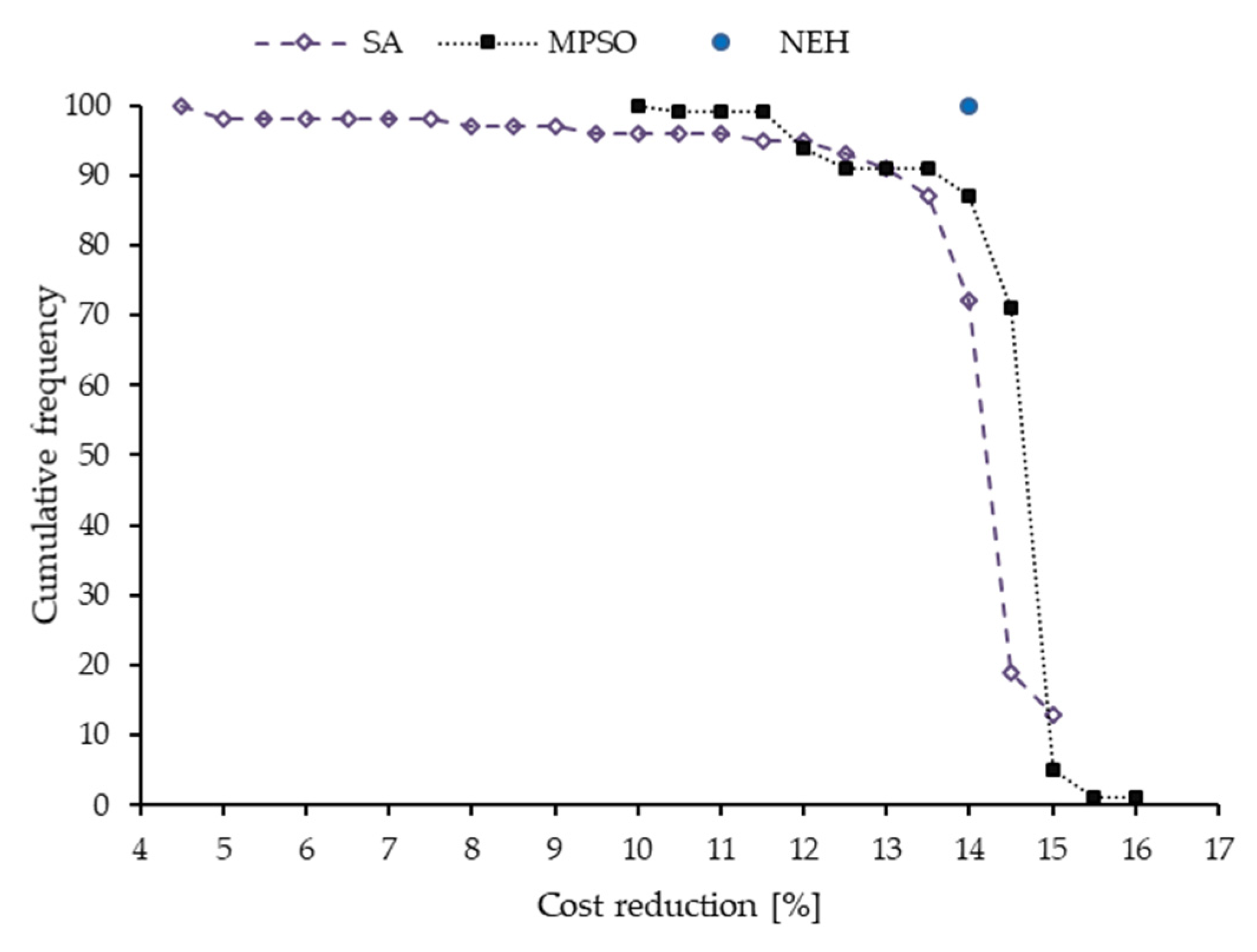
The optimization algorithms, except NEH, provide different results in different runs. Therefore, there is no certainty about delivering a best or nearly best solution always. Additionally, it is challenging to complete one optimization run within a reasonable time when the number of products, stages, and alternative resources are higher. Therefore, it is crucial to know the performance efficiency of optimization algorithms. To evaluate performance, the optimization was repeated 100 times for each of the algorithms, except NEH, to solve problem I.

In this study, the cumulative frequency was used to evaluate the performance i.e., how frequently an optimizer delivers best, better, good, and worst results. Cumulative frequency of 50 in a 10.0% cost reduction means an optimizer reduced cost by at least 10.0% in 50 runs.

3. Results and Discussion

3.1. Effect of Modification on the Performance of PSO

Figure 6a shows an example of the relative Euclidean distance between the current position of particles and the global best position $\left(g^{*}\right)$ from 100 test runs of MPSO, and Figure 6b represents the distribution of distance values at the 10th iteration, describing almost a normal distribution. However, from the raw Euclidean distance (Figure 6a), no clear pathway was observed. Therefore, the Savitzky Golay method was used to filter the data.

Figure 7 illustrates the Euclidean distance of particles from the global best position with Savitzky Golay filtering for PSO-A, PSO-B, and MPSO. It shows that at the initial phase, the distance of particles from the global best position $\left(g^{*}\right)$ was nearly the same for all the versions of PSO. In PSO-A, with the constant and lowest ration $C_1 / C_2$, 0.56, the particles searched solutions closer to the global best position.

PSO-B, in contrast, had constant ration $C_1 / C_2$ of 1.00, and particles were searching solutions always far from the best position. Despite PSO-A and PSO-B showing a rapid change in the first 10 iterations, a constant distance was observed till the end of the runtime. However, due to the change in the ratio of $C_1 / C_2$ over run time, MPSO had a good combination of searching solutions moderately far away at the initial phase, followed by an inclination toward the best position.

Figure 8 shows the cumulative frequency of standard PSO and MPSO to optimize the cost of different levels. In the worst cases of respective algorithms, MPSO provided a cost reduction of 10.0%, while for PSO-A and PSO-B, it was 7.5% and 6.5%, respectively. The figure shows that the possibility of giving the worst optimization results (<10.0%) by PSO-A is 3%, followed by PSO-B with 9%. However, MPSO showed no such cases in 100 test runs. MPSO outperformed PSO-A and PSO-B in the probability to obtain a better level of optimization results (at least 12.0% cost reduction). In 94 out of 100 runs, MPSO was able to reach this level while for PSO-A and PSO-B, it was 92 and 77, respectively. However, cost reductions by 14.0% or higher were found to be the most difficult level of optimization. At that level, PSO was outperformed by MPSO significantly, provided in 87 runs, which is 25 higher than PSO-A, and 33 higher than PSO-B.

Figure 9 shows the trend of searching for an improved solution during a run from PSO-A, PSO-B, and MPSO that turned into the corresponding best optimization results. It demonstrates that MPSO had the best optimization result with a reduction of cost by 16.3%.

Figure 10 depicts the convergence of the PSO variants calculated from the mean of the best optimization cost at different iterations. PSO-A had the worst mean cost reduction in the first 10 iterations of particles, while PSO-B and MPSO had a similar mean convergence.

However, the scenario changed over the next iterations as PSO-A showed a sharp improvement and outperformed PSO-B. MPSO showed the most consistency in improving the solution from the beginning to the end, which can be explained by the convergence rate. The convergence rate describes how the solutions were upgraded in terms of cost reduction by every iteration. The rate of the mean convergence of PSO-A, PSO-B, and MPSO is 0.27%, 0.26%, and 0.28%, respectively. In PSO-B, both cognitive and social velocities of particles in the swarm were equally weighted. According to this study, such configuration showed no visible improvements after the 25th iteration. In contrast, in PSO-A, cognitive velocity was constantly 1.8 times higher compared to the social velocity and outperformed PSO-B. MPSO was configured in a way that initially, the weight to social velocity was relatively higher and gradually decreased to give more strength to cognitive velocity. Such modifications in PSO were found to be efficient to obtain the best optimization results with a higher possibility.

Figure 11 represents the performance comparison of MPSO, SA, and NEH. It shows that NEH optimized the cost of production by 14.0%. However, NEH was outperformed by MPSO 87 times and by SA 72 times in 100 test runs. Moreover, SA provided the very worst quality optimization results with the lowest cost reduction of 4.5%, where MPSO had 10.0% at the worst level of performance. Therefore, it can be said that MPSO outperformed SA and NEH by solving the optimization problem most efficiently.

The best results from the optimized production schedules obtained by MPSO are described here. Figure 12 shows the comparison of idle time of only energy-consuming machines used for the production. It was observed that proper allocation of tasks among machines can reduce the overall idle time significantly. The results show that idle time for mixers, ovens, a fryer, and a slicer were reduced by 25%, 45%, 8%, 76%, and 38%, respectively, whereas for dividers it increased by 54%. The TIDT in the optimized schedule was reduced by 12%, and makespan by 30%.

Table 4. Cost calculation for the existing and optimized schedules.

	Makespan [min]	WTIDT	Total Cost	Cost Reduction [%]
Existing schedule	968	3110	4078	16.3%
Optimized schedule	675	2736	3411

shows the cost calculation for the best schedule obtained by MPSO. The optimized cost $(Cos{t}_{opt})$ and initial cost $\left(C_0\right)$ were calculated from the optimized and existing schedule respectively using Equation (1). WTIDT represents the cost due to the idle time of the machines calculated by using Equation (4).

3.2. Performance Comparison between MPSO and PSO from Literature

As a benchmark, problem II and constraints described by Hecker et al. [6] were taken into consideration. The authors found that the standard PSO performed slightly better than ant colony optimization in optimizing makespan. For better comparisons, the objective function was changed to a single objective to optimize makespan as the authors described. Moreover, instead of WTIDT, the comparison was on TIDT.

Figure 13 shows that the best makespan from the study was 8.4% [6], where for the proposed MPSO it was 8.7%. In 10 out of 21 runs, MPSO provided better optimization than the best performance of PSO. MPSO showed a possibility of 90% to optimize the makespan at least by 8.0%, while PSO showed only 47% possibility. The worst performance from MPSO was 7.6% of makespan reduction. The figure describes that there is a possibility (52%) that PSO cannot reach the worst performance of MPSO. In 11 out of 21 runs, PSO showed a relatively lower performance than the worst case of MPSO. However, optimizing one from makespan and TIDT may not be always cost-effective. It was observed that the optimized schedule with the objective of reducing makespan may have a higher TIDT, which causes high energy consumption. Contrarily, a schedule with optimized TIDT may have a higher makespan, meaning the production run time will be longer.

Figure 14 shows the effectiveness of the single objective optimized results. As makespan reduction was the only objective, TIDT was ignored by the optimization algorithm. The result shows that despite a higher makespan reduction, in some cases, the TIDT was increased, indicated by a negative TIDT [%]. In the worst scenario, the TIDT was increased by 10%, while makespan was reduced by 8%. Similar results were also obtained by Hecker et al. [6].

From the industrial perspective, it depends on how the makespan and TIDT influence the overall production cost which may vary from region to region and bakery to bakery. Therefore, the addition of a weighting factor for each machine may allow modifying the cost function to reflect the real production cost.

4. Conclusions and Outlook

The motivation of this study was to develop a task allocation model for production in bakery industries consisting of complex and mixed constraints, along with searching for an optimized schedule. The integration of many constraints, mainly to make feasible, increases the difficulty to optimize the production. However, the results demonstrated that an optimized schedule could still reduce the makespan and machine idle time of an existing production line significantly by performing heuristic and metaheuristic optimization algorithm.

Furthermore, the robustness and reliability of the optimization algorithms were examined. The study revealed that the convergence rate of PSO could be highly increased by adjusting the acceleration ratio to the best configuration using supporting parameters. Such modification in PSO could outperform standard PSO, SA, and NEH.

This study might be valuable for bakery industries and decision-making authorities to design an efficient bakery production system. A change in the arrangement e.g., addition of machines, employees, or changing the work plan of employees can be conformed to monitor the production efficiency before implementation in a real production line.

Several ideas deserve further investigation, such as the integration of more constraints that might occur in specific bakeries to provide customization opportunities to the bakery industry. Moreover, the application of other heuristic and meta-heuristic algorithms and a combination of their best features can be explored to find a robust optimizer.