Spiking Neural Membrane Computing Models

Abstract

As third-generation neural network models, spiking neural P systems (SNP) have distributed parallel computing capabilities with good performance. In recent years, artificial neural networks have received widespread attention due to their powerful information processing capabilities, which is an effective combination of a class of biological neural networks and mathematical models. However, SNP systems have some shortcomings in numerical calculations. In order to improve the incompletion of current SNP systems in dealing with certain real data technology in this paper, we use neural network structure and data processing methods for reference. Combining them with membrane computing, spiking neural membrane computing models (SNMC models) are proposed. In SNMC models, the state of each neuron is a real number, and the neuron contains the input unit and the threshold unit. Additionally, there is a new style of rules for neurons with time delay. The way of consuming spikes is controlled by a nonlinear production function, and the produced spike is determined based on a comparison between the value calculated by the production function and the critical value. In addition, the Turing universality of the SNMC model as a number generator and acceptor is proved.

1. Introduction

Membrane computing, an important branch of natural computing, is a computing model inspired by the structure, function, and behavior of biological cells. At present, there are three main types of membrane computing models: cell-like P system, tissue-like P system, and neural P system. In the past few years, research on neural P systems has mostly focused on spiking neural P systems, which is a type of computing model inspired by the processing of information in the form of spikes by neurons in biological neural networks. In 2006, Ionescu et al. first proposed the concept of spiking neural membrane systems [1], which have received extensive attention in recent years as a third-generation neural network model. Artificial neural networks are based on imitating the information processing function of the human brain nervous system, based on network topology to simulate the processing mechanism of the human brain nervous system towards complex information. It is a type that combines the understanding of biological neural networks with mathematical models to achieve powerful information processing capabilities, and it has a wide range of applications in pattern recognition, information processing, and image processing. We can find that both membrane computing and artificial neural networks are inspired by biological neural networks, and, in a certain sense, they are connected.

The SNP systems have accumulated rich research results in theory and application, especially in theoretical research. By changing the rules, objects, synapses, and structures to expand systems, many new SNP systems have been established. The changes in rules are mainly reflected in the form of the rules, such as SNP systems with white hole rules [2], SNP systems with communication rules [3], SNP systems with polarizations [4], asynchronous SNP systems [5], SNP systems with inhibitory rules [6], SNP systems with astrocytes [7], nonlinear SNP systems [8], and numerical SNP systems [9]. Inspired by the inhibitory spike effect of communication between neurons, the concept of the anti-spike was introduced, and a type of SNP system with anti-spike was proposed [10,11,12]. With expansions on synapses, there are systems such as SNP systems with weights on synapses [13], SNP systems with multiple channels [14], SNP systems with the rule on the synapse [15,16], and SNP systems with scheduled synapses [17,18]. The improvement of the structure mainly lies in making the structure of the membrane system dynamically changeable, for example, self-organizing SNP systems with variable synapses [19] and SNP systems with neuron division and budding [20].

SNP systems have a good network-distributed structure, a powerful parallel computing ability, dynamic characteristics, and nondeterminism. These characteristics mean the SNP systems have good application prospects in solving many practical problems. At present, some scholars have proven the feasibility of SNP systems to solve pattern recognition problems [21,22,23,24,25], combined with algorithms to solve optimization problems [26,27,28], clustering [29], automatic design [30], fault diagnosis [31,32,33,34], and perform arithmetic and logic operations [35,36,37,38], implemented by software and hardware [39,40].

At present, the research on membrane computing mainly focuses on theoretical research, and further research on its application is needed. Therefore, how to use membrane computing to solve practical application problems is not only an important topic in the field of membrane computing research, it also has important significance for the theoretical development of membrane computing and neural networks. Membrane computing is similar to artificial neural networks in many features; for example, they are both highly parallel. Therefore, some scholars are currently dedicated to combining membrane computing with neural networks. For example, according to the self-organizing and self-adaptive characteristics of the artificial neural network, SNP systems with a plastic structure have been proposed [41,42,43,44]. Inspired by Eckhorn’s neuron model, coupled neural P systems are proposed [45]. Inspired by the intersecting cortical model, dynamic threshold neural P systems have been proposed [46]. An application is the use of neural network and neural P systems for image processing [47,48,49,50]. It is notable that the combination of neural network and neural P systems is only a theoretical improvement based on a certain characteristic of neural networks or an improvement in rule structure based on the operation mechanism of a specific network model. This has certain research value and development prospects for the development of membrane computing, but these still need further research.

Therefore, both the theory and application of membrane computing need to be further expanded. Artificial neural networks are currently widely used in classification, image processing, and pattern recognition, but there are few studies on membrane computing dealing with these problems. If they can be combined, the theory and application research of membrane computing can be further expanded. In this paper, based on the structure of the neural network and data processing method, combining it with membrane computing, spiking neural membrane computing models (SNMC models) are proposed. SNMC models retain the distributed parallel computing of membrane computing and also have the method and structure of data processing by artificial neural networks, which provides a new dynamic evolution model and enriches the computing model for membrane computing.

Although SNP systems have made great progress in recent years, they still have some problems that can be improved, especially in data processing. In computer engineering and other fields of calculation, numerical information processing is important work. However, traditional SNP systems take the number of spikes as symbolic data, so it is difficult to process a large amount of numerical information. However, in the SNMC model, although the object is still spike, its production function can realize the processing of numerical information.

In this paper, inspired by the MP neuron model, SNMC models are proposed. The SNMC model contains two data units and rules with a production function. The data units are all real values. The function of rules is to control the activation of neurons. Additionally, the formulation of the rules is inspired by a nonlinear activation function. The main difference between the SNMC model and the artificial neural network is that the data flow of the SNMC model is completed by rules and objects. The artificial neural network is only calculated through mathematical models. The difference between the SNMC models and the existing SNP systems are as follows.

(1)

The forms of the rules are different; they contain the production functions. Additionally, each neuron contains two data units, including the input value and the threshold value. However, SNP systems contain the number of spikes in integer form.

(2)

The execution steps of the rules are different. When the rules start to be executed, SNMC models have the production and comparison steps.

(3)

The synapse weights of connecting neurons in SNMC models are divided into inhibitory synapses and excitatory synapses, and the corresponding weights are positive and negative. It can be explained in this manner: if the spike passes through the inhibitory synapse, the spike will be negatively charged.

The structure of the rest of this paper is as follows. In Section 2, we give the concepts of SNP systems and the MP model. In Section 3, the definition of a new type of neural membrane computing model, called the SNMC model, is given; a detailed explanation of the definition is also given, and the working process of the model is explained through an example. In Section 4, through a simulation of a register machine, the Turing universality of the SNMC model is proven in the generating mode and the accepting mode, respectively. Finally, conclusions and future work are given in Section 5.

2. Related Works

In this section, SNP systems and the general mathematical model of the neuron network are introduced. Moreover, some basic expressions of membrane computing are given.

2.1. Spiking Neural P Systems

Definition 1.

An SNP system with the degree$m\ge 1$is regarded as a tuple

$$\Pi =(O,{\sigma }_1,{\sigma }_2,\cdots ,{\sigma }_m,syn,in,out)$$

where

(1)

$O=\left\{a\right\}$ is the alphabet, and $a$ is a spike included in neurons;

(2)

$({\sigma }_1,{\sigma }_2,\cdots ,{\sigma }_m)$ represents $m$ neurons with the form ${\sigma }_i=(n_i,R_i)$, $1\le i\le m$, where

(a)

$n_i\ge 0$ is the number of spikes in neuron ${\sigma }_i$;

(b)

$R_i$ is the finite set of rules, including spiking rules and forgetting rules. The form of spiking rules is $E/a^c\to a^p;d$, $c\ge p\ge 1$, where $d$ indicates the time delay and $E$ indicates the regular expression over the alphabet $O$. The form of forgetting rules is $a^s\to \lambda$, $s\ge 1$. Additionally $\lambda$ indicates the neuron is empty, without spikes.

(3)

$syn\subseteq \{1,\cdots ,m\}\times \{1,\cdots ,m\}$ represents synapses that connect neurons. Additionally, $(i,j)\subseteq syn$($i\ne j$) indicates the synapse between neuron ${\sigma }_i$ and neuron ${\sigma }_j$, where;

(4)

$in$ is the input neuron;

(5)

$out$ is the output neuron.

An SNP system can be regarded as a digraph without self-circulation, denoted as $G(V,A)$. V is a set of vertices for neurons. A is the arc set for synapses. Spikes and rules are included in neurons, and the number of spikes changes according to the rules in the neuron. If the spiking rule activates, it means that the neuron contains at least $c$ spikes. Additionally, these $c$ spikes will be consumed and produce $p$ spikes that are sent to connected neurons after $d$ time units. In particular, the parameter $d$ refers to delay, which means that the neurons involved in the delay turn off and refuse to accept external spikes before $d$ time units. For instance, assume $d=2$ and the rule in neuron ${\sigma }_i$ fires at step $t$, then ${\sigma }_i$ is closed in steps $t$ and $t+1$. The neuron ${\sigma }_i$ reopens at step $t+2$ and receives spikes at the next step.

If the forgetting rule activates, it means $s$ spikes are removed from the neuron. The function of input neuron is reading spikes from the environment, and the function of the output neuron is outputting the results computed by the system.

The register machine has been shown to describe a set of recursive enumerable languages called NRE, which is equivalent to the computing power of the Turing machine. When proving the computational universality of various membrane systems below, the purpose of characterizing NRE is mainly achieved by simulating the register machine, which is denoted as a tuple, $M=(m,H,l_0,l_h,I)$. Among them, $m$ is the number of registers, $H$ is the instruction tag set, $l_0$ is the start instruction, $l_h$ is the halting instruction, and $I$ is the instruction set. It is notable that each element in $I$ corresponds to the element in $H$. The register machine $M$ contains the following three forms of instructions:

(1)

ADD instructions, such as $l_i:(ADD(r),l_j,l_k)$, mean that the number stored in register $r$ is increased by 1, and the next instruction is chosen $l_j$ or $l_k$ nondeterministically.

(2)

SUB instructions, such as $l_i:(SUB(r),l_j,l_k)$, generate two results according to the number in register $r$. If the value stored in register $r$ is greater than 0, the operation of subtracting 1 is performed, and the next instruction $l_j$ is executed. If the value stored in register $r$ is equal to 0, no operation is performed on $r$, and the next execution instruction is $l_k$.

(3)

Halting instruction $l_h:HALT$ is used to halt calculation.

2.2. Neural Network

From a biological point of view, a neuron can be regarded as a small processing unit. Additionally, the neural network of the brain is made up of many neurons connected in a certain way. The simplified mathematical model of neurons is shown in Figure 1. The representation of the model can be regarded as Formula (1), which indicates the sum of input of neuron $i$

$$a_i={\displaystyle \sum _j{w}_{ij}{x}_j}-b_i$$

(1)

where $w_{ij}$ is the weight between neuron $i$ and neuron $j$, $x_j$ is the input vector that comes from neuron $j$, and $b_i$ is the threshold of neuron $i$, the value of which can be set to positive or negative. In this way, it indicates that the neuron activates when the signal received by the neuron is greater than the threshold.

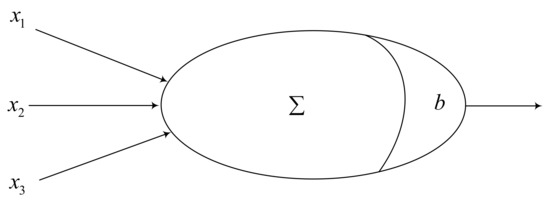
Figure 1. The structure of the MP neuron model.

This neuron model is called the MP neuron model, which is an abstract and simplified model constructed according to the structure and working principle of biological neurons. In our proposed models, we consider its activation function is a nonlinear function, which is the binary function shown as Formula (2)

$$y_i=\left\{\begin{array}{c}1,\hspace{1em}{a}_i>0\\ 0,\hspace{1em}{a}_i\le 0\end{array}\right.$$

(2)

3. Spiking Neural Membrane Computing Models

In this section, inspired by artificial neural networks, a new variant membrane computing model, called the spiking neural membrane computing model, is proposed. It is a combined model of neural network and spiking neural P systems and contains multiple neurons. Neurons are connected by synapses, and the synapses have weights, where the weights represent the relationship between neurons. To facilitate understanding and expression, we use an expression similar to SNP systems.

3.1. Definition

Definition 2.

The tuple of an SNMC model with a degree$m\ge 1$is represented as

$$\Pi =(O,N,W,syn,in,out)$$

where

(1)

$O=\left\{a\right\}$ is the alphabet, and $a$ refers to the spike included in neurons.

(2)

$N=\{{\sigma }_1,\cdots ,{\sigma }_m\}$ is the set of neurons, and neuron ${\sigma }_i$ has the form ${\sigma }_i=(u_i,b_i,p{f}_i,R_i)$, where

(a)

$u_i\in R$ is input data in neuron ${\sigma }_i$;

(b)

$b_i\in R$ is a threshold of neuron ${\sigma }_i$;

(c)

$p{f}_i$ is the production function, which is to compute the total real value of neuron ${\sigma }_i$. The total real value is the weighted sum of all inputs minus the threshold;

(d)

$R_i$ is the set of firing rules, with the form $E/a^{pf(u_i-b_i)\left|{}_0\right.}\to a^s;t_1,t_2$, $s\in \{0,1\}$. If $s=0$, neuron ${\sigma }_i$ is not producing spikes, denoted as $a^0=\lambda$.

(3)

$W$ is the weight on the synapse, which can be positive or negative. A positive weight means an excitatory synapse, and a negative weight means an inhibitory synapse.

(4)

$syn\subseteq \{1,2,\cdots m\}\times \{1,2,\cdots m\}\times W$ is the set of synapses.

(5)

$in$ and $out$ are the input neuron and the output neuron, respectively. The input neuron converts the input data into spikes containing real values. The output neuron outputs the input data as a binary string composed of 0 s and 1 s.

A spiking neural membrane computing model can be regarded as a digraph structure without self-circulation, where the nodes of the graph are represented by neurons, and the arcs represent the synaptic connections between neurons, as shown in Figure 2. The definition and description of SNMC models are given below. The neuron contains two kinds of data: a real input value and a threshold value. The way of transmitting data is determined by rules and synaptic connections.

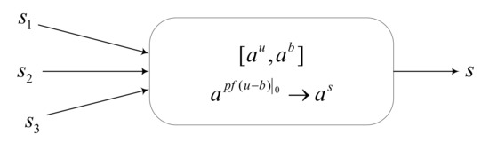
Figure 2. The neuronal structure of an SNMC model.

How the SNMC model works is explained here. There are two types of synapses: one is the inhibitory synapse, and the other is the excitatory synapse. This can be embodied by the value of weights, where a positive weight means an excitatory synapse, and a negative weight means an inhibitory synapse. It also indicates the relationship between neurons. For example, the weight between ${\sigma }_i$ and ${\sigma }_j$ is $w_{ij}=2$, which means the synapse between them is an excitatory synapse, and neuron ${\sigma }_j$ receives twice the value that neuron ${\sigma }_i$ outputs.

There are two types of data units in each neuron, including the input data unit and the threshold unit. The threshold can be 0, which means no threshold in neurons. It is notable that the neurons in our proposed model contain spikes with real values, which are real numbers. The input data $u_i$ of a neuron is the linking input data plus original data. The linking input data comes from the connected neurons, and the original data are that the neuron itself already exists. In this way, neuron ${\sigma }_i$ has a spike with real value $u_i$, which is the sum of the weighted values sent by the connected neurons plus the original values, such as Formula (3), where $w_{ij}$ is the weight between ${\sigma }_i$ and ${\sigma }_j$, $s_j$ is the output value of neuron ${\sigma }_j$, and ${\epsilon }_i$ is the original data of neuron ${\sigma }_i$.

$$u_i={\displaystyle \sum _j{w}_{ij}{s}_j}+{\epsilon }_i$$

(3)

For the convenience of calculation in this article, only integers are involved, which can be interpreted as “integer spikes” in this paper. For instance, the real value 2 is shown as $a^2$, which can be explained as two spikes in a neuron. Additionally, $a^{-2}$ is explained by two spikes with a negative charge in the neuron. A negatively charged spike can annihilate one spike.

The output state of the neuron is related to the rules. At each step, each neuron contains at least one firing rule, which is applied sequentially within the same neuron, but neurons work in parallel mode with each other. At a certain moment, if some neurons contain more than one rule that can be applied, they will nondeterministically choose one of the rules to apply. The way the rules are executed and interpreted is given below.

The rule contains two parts, including the production function and the outputting function. The production function is used to calculate the total real value of the current neuron, and the total effect on neuron ${\sigma }_i$ is the input data minus the threshold, which will cause the state change of neuron ${\sigma }_i$. In addition, the neuron has a critical value, which is set to 0. Therefore, the execution steps of rules are divided into three steps: production, comparison, and outputting.

(1)

Production step. When neuron ${\sigma }_i$ receives weighted spikes with real value $u_{1,i}(t_1),\hspace{0.17em}{u}_{2,i}(t_1),\cdots ,\hspace{0.17em}{u}_{k,i}(t_1)$ from connected $k$ neurons at time $t_1$, and the threshold is $b_i$, the production function works to calculate the total real value by Formula (4).

$$p{f}_i={\displaystyle \sum _j{u}_j}-b_i$$

(4)

(2)

Comparison step. In this step, the result $p{f}_i$ computed by Formula (4) is compared with the critical value 0. It determines whether the real value output of the next step is 1 or 0.

(3)

Outputting step. According to the result of the comparison step, if it has $p{f}_i>0$, then $s=1$, and the rule $E/a^{{\left.pf\left(u_i-b_i\right)\right|}_0}\to a;t_1,t_2$ can be applied to output a spike with the real value of 1. If it has $p{f}_i\le 0$, then $s=0$ and the rule $E/a^{pf(u_i-b_i)\left|{}_0\right.}\to \lambda ;t_1,t_2$ fires. Therefore, no spike can be sent to the connected neurons.

The firing of rules requires two conditions: (1) Assume the number of spikes contained in neuron ${\sigma }_i$ is $k$, $a^k$ belongs to the language set represented by the regular expression $E$, and the number of spikes $k$ contained in neuron ${\sigma }_i$ is greater than or equal to the number of spikes consumed, $u_i$, i.e., $k\ge u_i$. (2) The neuron can only be activated when it receives the signal sent by the connected neurons.

Additionally, $t_1$ and $t_2$ after the rule refers to time delay. $t_1$ means the time neuron receives spikes and $t_2$ represents the rule execution time (from the execution of the production steps to the outputting step). Before a delay of $t_1$ times, the neuron is in a closed state. If there is no delay, then the firing rule is abbreviated to $E/a^{pf(u_i-b_i)\left|{}_0\right.}\to a^s$. Moreover, the neuron fires and contains a spike with the real value of $u$; then, the real input value of the input unit is reset to 0, and the threshold unit is unchanged after the outputting step. In other words, once the rules fires in the neuron, the input value in the neuron is consumed. It is noted that if the input value of the SNMC model is a natural number, and there is no threshold in neurons and the weights are positive integers, then the SNP systems belong to a special case of our proposed SNMC models.

At each step, the configuration of the system $\Pi$ is composed of the real values of input units and threshold units of all neurons, denoted as $C_t\le u_1(t),b_1(t),\cdots ,u_m(t),b_m(t)>$, where $m$ is the number of neurons. The initial configuration is denoted as $C_0\le u_1(0),b_1(0),\cdots ,u_m(0),b_m(0)>$. With the application of firing rules, the configuration of the system $\Pi$ at a certain time is also changed. The transition from configuration at time $t$ to the configuration at time $t_1$ is denoted as $C_t\Rightarrow C_{t+1}$. When the calculation reaches a certain configuration and there is no rule that can be activated, then the calculation stops, and this configuration is denoted as $C_h$. The computational process of the system can be regarded as a transition of a series of configurations, which is ordered and finite, i.e., from the initial configuration to halting configuration $C_0\Rightarrow C_1\Rightarrow \cdots \Rightarrow C_h$.

When an SNMC model is working in a generating mode in the initial configuration, all the neurons in the model are empty except for neuron ${\sigma }_1$, which means that all registers are empty except for the number stored in Register 1. The calculation starts from instruction $l_0$, stops when the end instruction $l_h$ is reached, and then the number stored in Register 1 is the generated number. The calculation result is associated with the firing time of neuron ${\sigma }_{out}$, which is calculated by the time interval between the two nonzero values, that is, the time it takes neuron ${\sigma }_{out}$ to send the two spikes to the environment. Suppose that neuron ${\sigma }_{out}$ sends the spike to the environment for the first time at time $t_1$; the environment receives the second spike coming from ${\sigma }_{out}$ at time $t_2$, and then the calculation result is $t_2-t_1$. In addition, when an SNMC model works in the accepting mode, an input neuron ${\sigma }_{in}$ is added to read the values from the environment and all neurons are empty at the beginning. The number is fed into the system in the form of an encoded spike train, and it means the time interval between the two firings of ${\sigma }_{in}$ is the input number. For instance, the input number is $n$, $n\in N^{+}$, and it is encoded as a spike train ${10}^{n-1}1$, where 1 represents spike and 0 is empty. The interval between two spikes is $(n+1)-1=n$, which is the input number.

The family of all sets of numbers is denoted as $N_{\alpha }(\Pi )$, $\alpha \in \{2,acc\}$. When $\alpha =2$, $N_2(\Pi )$ represents the result of the system $\Pi$ calculation. Additionally, “2” indicates that only the first two firing times of neuron ${\sigma }_{out}$ are considered. When $\alpha =acc$, $N_{acc}(\Pi )$ is the set of all the accepted numbers by $\Pi$. The sets generated and accepted by SNMC models are denoted by $N_{\alpha }SNMC{(pf(2))}_m^{\beta }$, where $pf(2)$ means two variables contained in each production function, $m\ge 1$ is the number of neurons, and $\beta \ge 1$ is the number of rules. Notice that when the number of neurons cannot be counted, it is denoted by a symbol, $\ast$. In the following proof of the computing universality of SNMC models, the NRE, which is a family of numerically computable natural numbers, can be described mainly through simulating the register machine.

3.2. Illustrative Example

This example consists of 5 neurons and several synapses to explain the workflow of the system $\Pi$, as shown in Figure 3. Neuron ${\sigma }_1$ contains a real input value 2 and a threshold value 1, and it exists in the neuron in the form of spikes $[a^2,a]$. Suppose that at Time 1, neuron ${\sigma }_1$ fires since $pf=2-1=1>0$, and a spike is generated at Time 2, that is,$s=1$. Thus, neuron ${\sigma }_3$ receives two spikes from neuron ${\sigma }_1$. At Time 3, ${\sigma }_3$ generates one spike because its $pf$ value is 1. Additionally, neuron ${\sigma }_2$ contains two rules, of which one is selected for execution indeterminately. Hence, there are two cases that can happen depending on the rule selection in ${\sigma }_2$.

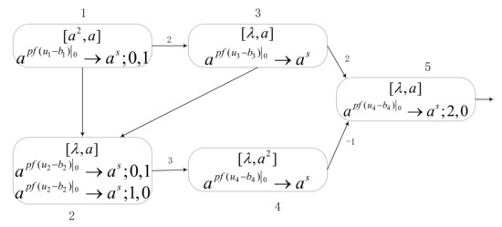
Figure 3. An example of the SNMC model. It is an explanation of the model workflow.

(1)

Assuming that the rule $a^{pf(u_2-b_2)\left|{}_0\right.}\to a^s;0,1$ is applied, neuron ${\sigma }_2$ receives a spike from ${\sigma }_1$ at Time 2, and then the production function executes at Time 3. The value $pf=1-1=0$ is obtained. Hence, at Time 4, neuron ${\sigma }_2$ produces and sends an empty to neuron ${\sigma }_4$. At the same time, neuron ${\sigma }_2$ also receives one spike from neuron ${\sigma }_3$; the rule $a^{pf(u_2-b_2)\left|{}_0\right.}\to a^s;1,0$ is used. Since its $pf$ value is 0, neuron ${\sigma }_2$ sends an empty to neuron ${\sigma }_4$. The neuron ${\sigma }_4$ has not received any spikes, so it produces empty at Time 5, and neuron ${\sigma }_5$ receives two spikes from neuron ${\sigma }_3$. At Time 6, its rule in neuron ${\sigma }_5$ fires and its $pf=2-1=1>0$, so it produces one spike and sends it out at the same time.

(2)

Assuming that the rule $a^{pf(u_2-b_2)\left|{}_0\right.}\to a^s;1,0$ is used, then neuron ${\sigma }_2$ is in the closed state before Time 3 and does not receive any spikes. At Time 3, the production function of neuron ${\sigma }_3$ performs and produces one spike to send to neurons ${\sigma }_2$ and ${\sigma }_5$. Thus, at Time 3, neuron ${\sigma }_2$ receives two spikes: one from neuron ${\sigma }_1$ and the other from neuron ${\sigma }_3$. At Time 4, since $pf=2-1-1>0$ in ${\sigma }_2$, it has $s=1$, and ${\sigma }_2$ produces a spike and sends it to neuron ${\sigma }_4$. Neuron ${\sigma }_4$ receives three spikes, and at Time 5, its producing function can be calculated as $pf=3-2=1>0$, so $s=1$. Meanwhile, neuron ${\sigma }_5$ receives two spikes from neuron ${\sigma }_3$ and one negative spike from neuron ${\sigma }_4$, so neuron ${\sigma }_5$ contains one spike. In this way, no spike is generated and sent out at Time 6 because of $pf=1-1=0$.

In order to conveniently display the changes of neurons at each time, a graph of configuration is given, as shown in Figure 4. The configuration in this figure is in the order of neuron ${\sigma }_1$, ${\sigma }_2$, ${\sigma }_3$, ${\sigma }_4$, and ${\sigma }_5$, and it is composed of the input unit and the threshold unit with the form of $C\le u_1,b_1,u_2,b_2,u_3,b_3,u_4,b_4,u_5,b_5>$. When rules are still performing at a certain moment, the corresponding spikes are considered not to be consumed completely, denoted as “$u_i{}^{\prime }$”.

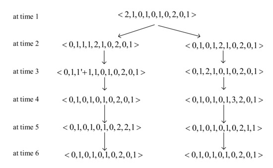
Figure 4. The configuration of the example at each time.

4. Turing Universality of SNMC Models

In this section, the computational power of SNMC models is proved as number generators and acceptors, respectively.

4.1. Generating Mode

In generating mode, the most important neuron ${\sigma }_{out}$ is contained. In this way, the Turing universality of SNMC models as a generator is investigated by simulating three instructions, including the ADD instruction, the SUB instruction, and the halt instruction. Thus, three modules, named ADD, SUB, and FIN modules, are used for the simulation. Assume that each neuron contains a certain initial threshold. It is stipulated that each neuron corresponding to an instruction has an initial threshold $a$, and each neuron corresponding to the register has an initial threshold $a$.

Theorem 1.

$N_{2}SNMC{(pf(2))}_{\ast }^2=NRE$.

Proof of Theorem 1.

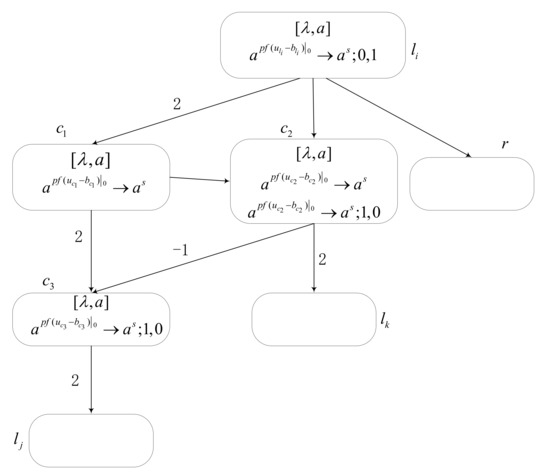
Module ADD is used to simulate ADD instructions $l_i:(ADD(r),l_j,l_k)$, as shown in Figure 5. When register $r$ is increased by one, the spike is transmitted indeterminately to $l_j$ or $l_k$. Assume that the configurations of the module ADD $C_t\le u_1,b_1,u_2,b_2,\dots ,u_6,b_6>$ is associated with six neurons ${\sigma }_{l_i}$, ${\sigma }_{c_1}$, ${\sigma }_{c_2}$,${\sigma }_{c_3}$, ${\sigma }_{l_j}$ and ${\sigma }_{l_k}$, respectively. Assume neuron ${\sigma }_{l_i}$ receives two spikes at time $t$, and the configuration of time $t$ is $C_t\le 2,1,0,1,0,1,0,1,0,1,0,1>$. At time $t+1$, the rule in ${\sigma }_{l_i}$ fires and the production function starts to compute. It has $pf=2-1=1>0$, thus neuron ${\sigma }_{l_i}$ sends the produced spike to neurons ${\sigma }_{c_1}$, ${\sigma }_{c_2}$ and ${\sigma }_r$ respectively, at time $t+2$. There are two rules within neuron ${\sigma }_{c_2}$, and the application of one of them is indeterminately selected. Therefore, two cases happen.

Figure 5. Module ADD. Its function is to Simulate ADD instruction $l_i:(ADD(r),l_j,l_k)$.

(1)

If the rule $a^{pf(u_2-b_2)\left|{}_0\right.}\to a^s$ is applied, neuron ${\sigma }_{c_1}$ receives two spikes and ${\sigma }_{c_2}$ receives one spike at time $t+2$. The configuration becomes $C_{t+2}\le 0,1,2,1,1,1,0,1,0,1,0,1>$. In neuron ${\sigma }_{c_1}$, it has $pf=2-1=1>0$ and sends one spike to ${\sigma }_{c_2}$ and ${\sigma }_{c_3}$ at time $t+3$. But due to the delay of one time in ${\sigma }_{c_3}$, neuron ${\sigma }_{c_3}$ receives the spike at the next time. Thus, the configuration of time $t+3$ is $C_{t+3}\le 0,1,0,1,1,1,0,1,0,1,0,1>$. At time $t+4$, the rule $a^{pf(u_2-b_2)\left|{}_0\right.}\to a^s;1,0$ fires and the production result in neuron ${\sigma }_{c_2}$ is $pf=1-1=0$, such that the neuron produced empty, with $s=0$ in the outputting step. In this way, neuron ${\sigma }_{l_k}$ is empty. Since the time delay in neuron ${\sigma }_{c_3}$, ${\sigma }_{c_3}$ only receives the spikes sent by neurons ${\sigma }_{c_2}$ and ${\sigma }_{c_1}$ at time $t+4$, so neuron ${\sigma }_{c_3}$ receives two spikes from ${\sigma }_{c_1}$ in total and $C_{t+4}\le 0,1,0,1,0,1,2,1,0,1,0,1>$. Calculate the $pf$ value $pf=2-1>0$, and one spike is generated. Therefore, neuron ${\sigma }_{lj}$ receives two spikes at time $t+5$ and $C_{t+5}\le 0,1,0,1,0,1,0,1,2,1,0,1>$.

(2)

If the rule $a^{pf(u_2-b_2)\left|{}_0\right.}\to a^s;1,0$ in neuron ${\sigma }_{c_2}$ is activated, then at time $t+2$, since there is the time delay in ${\sigma }_{c_2}$, only neuron ${\sigma }_{c_1}$ receives two spikes and neuron ${\sigma }_r$ receives one spike. The configuration of time $t+2$ is $C_{t+2}\le 0,1,1,1,0,1,0,1,0,1,0,1>$. The $pf$ value in neuron ${\sigma }_{c_1}$ is 1, which is greater than 0; thus, ${\sigma }_{c_1}$ sends out a spike at time $t+3$. Thus, neuron ${\sigma }_{c_2}$ receives two spikes sent by neurons ${\sigma }_{l_i}$ and ${\sigma }_{c_1}$ at time $t+3$, and $C_{t+3}\le 0,1,0,1,2,1,0,1,0,1,0,1>$. At the next time, neuron ${\sigma }_{l_k}$ receives two spikes sent by neuron ${\sigma }_{c_2}$. Additionally, neuron ${\sigma }_{c_3}$ receives two spikes from ${\sigma }_{c_1}$ and one spike with a negative charge from neuron ${\sigma }_{c_2}$, so neuron ${\sigma }_{c_3}$ has one spike at this time, and the configuration is $C_{t+4}\le 0,1,0,1,0,1,1,1,0,1,0,1>$. Therefore, no spike is sent to neuron ${\sigma }_{lj}$ in time $t+5$ because of $pf=1-1<0$ in ${\sigma }_{c_3}$ and $C_{t+5}\le 0,1,0,1,0,1,0,1,0,1,2,1>$.

The module SUB, as shown in Figure 6, is used to simulate the SUB instruction in the register machine. The configuration of the module SUB is $C_t\le u_1,b_1,\dots u_7,b_7>$; they correspond to the number of input units and threshold units of neurons ${\sigma }_{l_i}$, ${\sigma }_{v_1}$, ${\sigma }_r$, ${\sigma }_{v_2}$, ${\sigma }_{v_3}$, ${\sigma }_{l_j}$ and ${\sigma }_{l_k}$. Assume that neuron ${\sigma }_{l_i}$ receives two spikes at time $t$, and the configuration is $c_t\le 2,1,0,1,x,1,0,1,0,1,0,1,0,1>$. At time $t+1$, the production function starts to calculate a $pf$ value that is equal to 1 (greater than 0), so one spike is generated at time $t+2$ and sent to ${\sigma }_{v_1}$ and ${\sigma }_r$. At time $t+2$, neuron ${\sigma }_{v_1}$ receives two spikes, and neuron ${\sigma }_r$ receives one spike, but it is unknown whether there is empty in neuron ${\sigma }_r$. According to the number of spikes contained in ${\sigma }_r$, the operation results are divided into the following two cases:

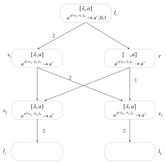
Figure 6. Module SUB. Its function is to simulate SUB instruction $l_i:(SUB(r),l_j,l_k)$.

(1)

If register $r$ of register machine $M$ stores a number $n>0$, it means that neuron ${\sigma }_r$ contains at least one spike. At time $t+2$, neuron ${\sigma }_r$ contains at least two spikes, and so $C_{t+2}\le 0,1,2,1,n+1,1,0,1,0,1,0,1,0,1>$. As its $pf$ value is 1>0, one spike is generated and sent to neurons ${\sigma }_{v_2}$ and ${\sigma }_{v_3}$, respectively, at time $t+3$. At the same time, neuron ${\sigma }_{v_1}$ generates one spike since $pf=2-1=1>0$. Thus, neuron ${\sigma }_{v_2}$ receives two spikes, one from ${\sigma }_r$ and the other from ${\sigma }_{v_1}$, and ${\sigma }_{v_3}$ receives one spike because one negatively charged spike and one spike are annihilated. The configuration of time $t+3$ is $C_{t+3}\le 0,1,0,1,0,1,2,1,1,1,0,1,0,1>$. At the next time, since $pf=2-1=1>0$ of neuron ${\sigma }_{v_2}$, a spike is generated and two spikes are sent to ${\sigma }_{l_j}$. Additionally, the $pf$ value of neuron ${\sigma }_{v_3}$ is 0, so no spike is generated; then, neuron ${\sigma }_{l_k}$ is empty. In this way, the configuration of time $t+4$ is $C_{t+4}\le 0,1,0,1,0,1,0,1,0,1,2,1,0,1>$.

(2)

Suppose that no number is stored in register $r$ at the initial time; that is, neuron ${\sigma }_r$ is empty. At time $t+2$, one spike from ${\sigma }_{l_i}$ is received by ${\sigma }_r$, and the rule fires. Thus, the configuration is $C_{t+2}\le 0,1,2,1,1,1,0,1,0,1,0,1,0,1>$. Since there is only one spike in ${\sigma }_r$, and its $pf=1-1=0$, neuron ${\sigma }_r$ produces no spike at time $t+3$. Meanwhile, the neuron ${\sigma }_{v_2}$ receives one spike from ${\sigma }_{v_1}$ and ${\sigma }_{v_3}$ receives two spikes from ${\sigma }_{v_1}$. The configuration of time $t+3$ is $C_{t+3}\le 0,1,0,1,0,1,1,1,2,1,0,1,0,1>$. At time $t+4$, the rule in ${\sigma }_{v_2}$ is applied, and the calculation $pf=1-1=0$, so no spike is generated. Additionally, according to the rule, ${\sigma }_{v_3}$ generates one spike and neuron ${\sigma }_{l_k}$ obtains two spikes. Therefore, neuron ${\sigma }_{l_k}$ has one spike and neuron ${\sigma }_{l_j}$ is empty. In this way, $C_{t+4}\le 0,1,0,1,0,1,0,1,0,1,0,1,2,1>$.

It is notable that despite that it is possible to have multiple SUB instructions operating on the same register, no incorrect simulation of $M$ caused by the interference among SUB modules in $\Pi$ takes place. Assume that SUB instructions $l_i$ and ${l^{\prime }}_i$ share the same register $r$, so when the instruction $l_i$ works, we need to ensure that the work of instruction ${l^{\prime }}_i$ will not be affected in the next work. Assume that the neurons connected to register $r$ in instruction ${l^{\prime }}_i$ have ${{\sigma }^{\prime }}_{v_2}$ and ${{\sigma }^{\prime }}_{v_3}$, which correspond to ${\sigma }_{v_2}$ and ${\sigma }_{v_3}$ shown in Figure 6. According to the simulation of the above module SUB, when there is no number stored in register $r$, neuron ${\sigma }_r$ does not generate any spike, so it will not affect instruction ${l^{\prime }}_i$. When register $r$ is not empty, then neuron ${\sigma }_r$ produces one spike. After passing through the synapse, neuron ${{\sigma }^{\prime }}_{v_2}$ receives one spike and neuron ${{\sigma }^{\prime }}_{v_3}$ receives a spike with a negative charge. According to the rules of neurons ${{\sigma }^{\prime }}_{v_2}$ and ${{\sigma }^{\prime }}_{v_3}$, their $pf$ value does not exceed 0, so no spike is generated. Therefore, instruction ${l^{\prime }}_i$ is not affected when instruction $l_i$ is simulated. In this way, the simulation of module SUB is proven correct.

The function of module FIN is to output the computational result (shown in Figure 7). Suppose that the number in Register 1 is $n$, that is, there are $n$ spikes in neuron ${\sigma }_1$. Additionally, neurons ${\sigma }_{l_h}$ and ${\sigma }_{out}$ contain a spike, respectively. Suppose that at time $t$, neuron ${\sigma }_{l_h}$ receives two spikes. As shown in Figure 7, we can see that the configuration is $C_t\le 2,1,0,1,0,1,0,1,n,1,0,0,1,1>$. Therefore, at time $t+1$, from the $pf$ value of ${\sigma }_{l_h}$ ($pf=2-1=1>0$), one spike is generated and sent to neurons ${\sigma }_{h_1}$ and ${\sigma }_{h_2}$. Neurons ${\sigma }_{h_1}$ and ${\sigma }_{h_2}$ both receive two spikes, and their rules are activated. Since the $pf$ values of ${\sigma }_{h_1}$ and ${\sigma }_{h_2}$ are $pf=2-1=1>0$, at time $t+2$, both neurons ${\sigma }_{h_1}$ and ${\sigma }_{h_2}$ generate one spike. Neurons ${\sigma }_{h_3}$ and ${\sigma }_{h_2}$ both receive two spikes from neuron ${\sigma }_{h_1}$, and neuron ${\sigma }_{h_1}$ also receives two spikes from ${\sigma }_{h_2}$. Hence, at time $t+3$ until the calculation stops, neurons ${\sigma }_{h_1}$ and ${\sigma }_{h_2}$ will always repeat the operation as at time $t+2$. At time $t+3$, the rule of neuron ${\sigma }_{h_3}$ is activated, and it has $pf=2-1=1>0$, so one spike is sent to neurons ${\sigma }_{out}$ and ${\sigma }_1$, respectively. Neuron ${\sigma }_{out}$ contains two spikes. Thus, at time $t+4$, according to the rule in ${\sigma }_{out}$, one spike can be generated and sent to the environment. At the same time, neuron ${\sigma }_{out}$ receives a spike obtained from neuron ${\sigma }_{h_3}$. It is worth noting that neuron ${\sigma }_{h_3}$ always sends one spike every time after time $t+3$ to neuron ${\sigma }_{out}$ and ${\sigma }_1$ until the calculation stops.

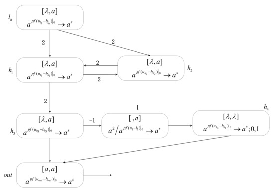
Figure 7. Module FIN. Its function is to output the computation result.

At time $t+3$, neuron ${\sigma }_1$ receives a spike with a negative charge. Hence, neuron ${\sigma }_1$ contains $n-1$ spikes at this time. However, according to the rule in neuron ${\sigma }_1$, the rule can fire if and only if the number of spikes in neuron ${\sigma }_1$ is not more than 2. Hence, until time $t+n$, when neuron ${\sigma }_1$ contains only two spikes, the rule is activated. At time $t+n+1$, since $pf=1>0$ in neuron ${\sigma }_1$, it generates a spike and sends it to neuron ${\sigma }_{h_4}$. At the next time, the rule of ${\sigma }_{h_4}$ fires. Since its $pf$ value is greater than 0 and the rule execution time has a one-step delay, one spike is generated and sent to neuron ${\sigma }_{out}$ at time $t+n+3$. At this time, neuron ${\sigma }_{out}$ also gets a spike from neuron ${\sigma }_{h_3}$, so it contains two spikes. Therefore, at time $t+n+4$, neuron ${\sigma }_{out}$ generates one spike and sends it to the environment. The calculation result of the SNMC model is defined as the time interval for the output neuron to send the first two nonzero values to the environment, that is, $t+n+4-\left(t+4\right)=n$ which is consistent with number $n$ stored in Register 1. Therefore, the FIN module can output the calculation result correctly.

In this way, the computation power of SNMC models in generating mode is investigated by simulating the register machine correctly through three modules. □

4.2. Accepting Mode

The computational power of an SNMC model is obtained by simulating the deterministic register machine in the accepting mode. We need to construct an SNMC model, including module INPUT, module SUB, and module ADD’, to simulate the deterministic register machine. Module SUB is the same as that in the generating mode, and we will not prove it in this part. Additionally, module ADD’ simulates the deterministic ADD instruction $l_i:(ADD(r),l_j)$.

Theorem 2.

$N_{acc}SNMC{(pf(2))}_{\ast }^2=NRE$.

Proof of Theorem 2.

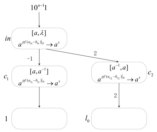
We only need to prove that module INPUT and module ADD can simulate the register machine. The function of module INPUT is to read the number encoded into a spike train into the model, as shown in Figure 8. Assume that number $n$ is to be read into the SNMC model by module INPUT. Firstly, encode $n$ into a spike train ${10}^{n-1}1$, where the time interval between two spikes is $n$. When input neuron ${\sigma }_{in}$ reads the symbol 1, it means that input value $u$ is 1, and when the read symbol is 0, it means input value $u$ is 0. Then, use module INPUT to store the number in Register 1. If Register 1 stores number $n$, it corresponds to neuron ${\sigma }_r$ receiving $n$ spikes.

Figure 8. Module INPUT. Its function is to read the spike train to model $\Pi$.

At the initial moment, there is one spike in neuron ${\sigma }_{in}$, one spike in ${\sigma }_{c_1}$, and one spike with a negative charge in ${\sigma }_{c_2}$, i.e., the initial configuration is $C_0\le 1,0,1,-1,-1,1,0,1,0,1>$. Suppose that at time $t$, neuron ${\sigma }_{in}$ receives the first spike from the environment. Thus, there are two spikes in ${\sigma }_{in}$. According to the rule $a^{pf(u_{in}-b_{in})\left|{}_0\right.}\to a^s$, the $pf$ value is equal to $2>0$, so a spike is generated. At time $t+1$, neuron ${\sigma }_{c_1}$ receives one spike with a negative charge, which annihilates the spike it contains. Hence, there is no spike in ${\sigma }_{c_1}$. According to the rule $a^{pf(u_{c_1}-b_{c_1})\left|{}_0\right.}\to a^s$, calculate the $pf$ value and $pf=0+1=1>0$. Hence, ${\sigma }_{c_1}$ produces one spike and sends it to neuron ${\sigma }_1$ at the next time. Neuron ${\sigma }_{c_2}$ also receives two spikes from ${\sigma }_{in}$ at time $t+1$, one of which is annihilated by the negatively charged spike. At this time, ${\sigma }_{c_2}$ has one spike. Additionally, calculate $pf=1-1=0$, so that neuron ${\sigma }_{c_2}$ generates empty at time $t+2$. Simultaneously, neuron ${\sigma }_{in}$ receives the empty (0) from the environment and sends the empty to neurons ${\sigma }_{c_1}$ and ${\sigma }_{c_2}$ according to its rule.

Therefore, at time $t+2$, neuron ${\sigma }_{c_1}$ is activated again, and its $pf=0+1=1>0$. Thus, ${\sigma }_{c_1}$ produces one spike and sends it to neuron ${\sigma }_1$. At the next time $t+n-1$, neuron ${\sigma }_{in}$ always accepts the empty, so neuron ${\sigma }_1$ receives $n$ spikes until time $t+n$. At time $t+n$, ${\sigma }_{in}$ obtains the second spike. Thus, according to the value $pf=1-0=1>0$, ${\sigma }_{in}$ produces one spike. In this way, ${\sigma }_{c_1}$ receives one spike with a negative charge, and ${\sigma }_{c_2}$ receives two spikes. At time $t+n+1$, neuron ${\sigma }_{c_1}$ fires, and its $pf=-1+1=0$, hence no spike is generated. Meanwhile, according to the rule in neuron ${\sigma }_{c_2}$ which is $pf=2-1=1>0$, a spike is produced and two spikes are sent to neuron ${\sigma }_{l_0}$. So far, the module INPUT simulation is completed.

The module ADD’, used to simulate deterministic ADD instruction $l_i:(ADD(r),l_j)$, is shown in Figure 9. When neuron ${\sigma }_{l_i}$ receives two spikes, the produced one spike is transmitted to neuron ${\sigma }_{l_j}$ because of $pf=2-1=1>0$; hence, neuron ${\sigma }_{l_j}$ receives two spikes and neuron ${\sigma }_r$ also gets one spike from neuron ${\sigma }_{l_i}$. Therefore, the operation of increasing by 1 to register $r$ is successfully simulated by module ADD’.

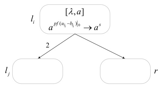
Figure 9. Module ADD’. Its function is to simulate deterministic ADD instruction $l_i:(ADD(r),l_j)$.

Based on the above proof, it is determined that the register machine can be correctly simulated by the SNMC model working in the accepting mode. Therefore, $N_{acc}SNMC{(pf(2))}_{\ast }^2=NRE$. □

5. Conclusions

Inspired by the SNP systems and artificial neural networks, this paper presents a new membrane computing model called the spiking neural membrane computing model. The model is composed of multiple neurons and connected synapses. The weights on the synapses represent the relationship between the neurons. According to the types of synapses, weights can be either positive or negative. If the synapse is inhibitory, the weight is negative. If the synapse is excitatory, a positive weight value denotes it. Each neuron contains two data units: the input value unit and the threshold unit, both of which exist in the form of spikes. In this model, the activation of rules in neurons requires two conditions. One is to meet the conditions generated by the regular expression, and the other is that the neuron can only be activated when it receives signals from the connected neurons.

The operation of the rule needs to be divided into three stages: production step, comparison step, and outputting step. Note that when the generated positive real value is transmitted to the neuron through the inhibitory synapse, the neuron receives a negative value; this means that there is a spike with a negative charge in the neuron. A spike with a negative charge and a spike with a positive charge can cancel each other out. In addition, we also proved the computing power of the SNMC model through Theorems 1 and 2. When the model is in the generating mode, the Turing universality of the SNMC model as a number generator is proven by simulating the nondeterministic register machine. Additionally, the Turing universality of the SNMC model as a number acceptor is proven by simulating a deterministic register machine.

The following are the advantages of the SNMC model:

• The weight and threshold values are introduced into the SNMC model, and the rule mechanism is improved compared with the SNP system so that the model combines the advantages of membrane computing and neural networks and can extend the application when processing real value information in particular.
• The rules of the SNMC model involve production function, and the calculation method of production function originates from the data processing method of neural networks, so the effective combination of the SNMC model and algorithms can be realized in the future.
• The computing power of the SNMC model has been proven, and it is a kind of Turing universal computational model.

The SNMC model extends the current SNP systems and comprehensively considers the relevant elements of the current SNP systems, such as time delay, threshold, and weight. The way of data processing in SNMC models makes the development of SNP systems more possible. We found that if the potential value of the SNMC model is a natural number, there is no threshold and weights are only positive integers; then, most of the currently existing SNP systems belong to a special case of our proposed SNMC model. The main difference between SNMC models and current SNP systems lies in the operating mechanism of rules. For example, the SNMC model is compared with SNP systems with weights and thresholds (WTSNP) [51]. They have different forms of rules, roles of thresholds, and operation mechanisms of rules. Additionally, the main difference with the numerical SNP system (NSNP) [9] is that the NSNP is embedded into the SNP system as the form of rule of the numerical P system and its object is not a spike. The firing rules also operate differently. In the SNMC model, the potential value is consumed in the form of spikes, and two results are produced, 0 or 1, according to the comparison results of the production function. Additionally, the SNMC model works by mapping the production function to an activation function.

The main difference between the SNMC model and artificial neural networks is that the data flow of the SNMC model is completed by rules and objects. Artificial neural networks are only calculated through mathematical models. The proposed SNMC model not only retains the distributed parallel computing of membrane computing but also has the method and structure of neural networks for data processing. Therefore, the model can be used in the future to deal with certain practical problems and expand the application of membrane computing. For example, further research can be carried out on image processing and algorithm design.

References

- Ionescu, M.; Păun, G.; Yokomori, T. Spiking neural P systems. Fundam. Inform. 2006, 71, 279–308. [Google Scholar]
- Song, T.; Gong, F.; Liu, X.; Zhao, Y.; Zhang, X. Spiking neural P systems with white hole neurons. IEEE Trans. NanoBiosci. 2016, 15, 666–673. [Google Scholar] [CrossRef]
- Wu, T.; Bîlbîe, F.-D.; Păun, A.; Pan, L.; Neri, F. Simplified and yet Turing universal spiking neural P systems with communication on request. Int. J. Neural Syst. 2018, 28, 1850013. [Google Scholar] [CrossRef]
- Wu, T.; Pan, L. The computation power of spiking neural P systems with polarizations adopting sequential mode induced by minimum spike number. Neurocomputing 2020, 401, 392–404. [Google Scholar] [CrossRef]
- Song, X.; Peng, H.; Wang, J.; Ning, G.; Sun, Z. Small universal asynchronous spiking neural P systems with multiple channels. Neurocomputing 2020, 378. [Google Scholar] [CrossRef]
- Peng, H.; Li, B.; Wang, J.; Song, X.; Wang, T.; Valencia-Cabrera, L.; Pérez-Hurtado, I.; Riscos-Núñez, A.; Pérez-Jiménez, M.J. Spiking neural P systems with inhibitory rules. Knowl. Based Syst. 2020, 188, 105064. [Google Scholar] [CrossRef]
- Aman, B.; Ciobanu, G. Spiking Neural P Systems with Astrocytes Producing Calcium. Int. J. Neural Syst. 2020, 30, 2050066. [Google Scholar] [CrossRef]
- Peng, H.; Lv, Z.; Li, B.; Luo, X.; Wang, J.; Song, X.; Wang, T.; Pérez-Jiménez, M.J.; Riscos-Núñez, A. Nonlinear spiking neural P systems. Int. J. Neural Syst. 2020, 30, 2050008. [Google Scholar] [CrossRef]
- Wu, T.; Pan, L.; Yu, Q.; Tan, K.C. Numerical Spiking Neural P Systems. IEEE Trans. Neural Netw. Learn. Syst. 2020. [Google Scholar] [CrossRef]
- Pan, L.; Păun, G. Spiking neural P systems with anti-spikes. Int. J. Comput. Commun. Control 2009, 4, 273–282. [Google Scholar] [CrossRef]
- Wu, T.; Zhang, T.; Xu, F. Simplified and yet Turing universal spiking neural P systems with polarizations optimized by anti-spikes. Neurocomputing 2020, 414, 255–266. [Google Scholar] [CrossRef]
- Song, X.; Wang, J.; Peng, H.; Ning, G.; Sun, Z.; Wang, T.; Yang, F. Spiking neural P systems with multiple channels and anti-spikes. Biosystems 2018, 169, 13–19. [Google Scholar] [CrossRef]
- Pan, L.; Zeng, X.; Zhang, X.; Jiang, Y. Spiking Neural P Systems with Weighted Synapses. Neural Process. Lett. 2012, 35, 13–27. [Google Scholar] [CrossRef]
- Peng, H.; Yang, J.; Wang, J.; Wang, T.; Sun, Z.; Song, X.; Luo, X.; Huang, X. Spiking neural P systems with multiple channels. Neural Netw. 2017, 95, 66–71. [Google Scholar] [CrossRef]
- Cabarle, F.G.C.; de la Cruz, R.T.A.; Cailipan, D.P.P.; Zhang, D.; Liu, X.; Zeng, X. On solutions and representations of spiking neural P systems with rules on synapses. Inf. Sci. 2019, 501, 30–49. [Google Scholar] [CrossRef]
- Jiang, S.; Fan, J.; Liu, Y.; Wang, Y.; Xu, F. Spiking neural P systems with polarizations and rules on synapses. Complexity 2020, 2020, 8742308. [Google Scholar] [CrossRef]
- Cabarle, F.G.C.; Adorna, H.N.; Jiang, M.; Zeng, X. Spiking neural P systems with scheduled synapses. IEEE Trans. NanoBiosci. 2017, 16, 792–801. [Google Scholar] [CrossRef]
- Bibi, A.; Xu, F.; Adorna, H.N.; Cabarle, F.G.C. Sequential Spiking Neural P Systems with Local Scheduled Synapses without Delay. Complexity 2019, 2019, 7313414. [Google Scholar] [CrossRef]
- Wang, X.; Song, T.; Gong, F.; Zheng, P. Computational power of spiking neural P systems with self-organization. Sci. Rep. 2016, 6, 27624. [Google Scholar] [CrossRef]
- Pan, L.; Păun, G.; Pérez-Jiménez, M.J. Spiking Neural P systems with neuron division and budding. Sci. China Inf. Sci. 2011, 54, 1596–1607. [Google Scholar] [CrossRef]
- Song, T.; Pang, S.; Hao, S.; Rodríguez-Patón, A.; Zheng, P. A parallel image skeletonizing method using spiking neural P systems with weights. Neural Process. Lett. 2019, 50, 1485–1502. [Google Scholar] [CrossRef]
- Gou, X.; Liu, Q.; Rong, H.; Hu, M.; Pirthwineel, P.; Deng, F.; Zhang, X.; Yu, Z. A Novel Spiking Neural P System for Image Recognition. Int. J. Unconv. Comput. 2021, 16, 121–139. [Google Scholar]
- Ma, T.; Hao, S.; Wang, X.; Rodriguez-Paton, A.A.; Wang, S.; Song, T. Double Layers Self-Organized Spiking Neural P Systems with Anti-Spikes for Fingerprint Recognition. IEEE Access 2019, 7, 177562–177570. [Google Scholar] [CrossRef]
- Song, T.; Pan, L.; Wu, T.; Zheng, P.; Wong, M.L.D.; Rodriguez-Paton, A. Spiking Neural P Systems with Learning Functions. IEEE Trans. NanoBiosci. 2019, 18, 176–190. [Google Scholar] [CrossRef] [PubMed]
- Chen, Z.; Zhang, P.; Wang, X.; Shi, X.; Wu, T.; Zheng, P. A computational approach for nuclear export signals identification using spiking neural P systems. Neural Comput. Appl. 2018, 29, 695–705. [Google Scholar] [CrossRef]
- Zhu, M.; Yang, Q.; Dong, J.; Zhang, G.; Gou, X.; Rong, H.; Paul, P.; Neri, F. An Adaptive Optimization Spiking Neural P System for Binary Problems. Int. J. Neural Syst. 2020, 31, 2050054. [Google Scholar] [CrossRef]
- Ramachandranpillai, R.; Arock, M. An adaptive spiking neural P system for solving vehicle routing problems. Arab. J. Sci. Eng. 2020, 45, 2513–2529. [Google Scholar] [CrossRef]
- Zein, M.; Adl, A.; Hassanien, A.E. Spiking neural P grey wolf optimization system: Novel strategies for solving non-determinism problems. Expert Syst. Appl. 2019, 121, 204–220. [Google Scholar] [CrossRef]
- Kong, D.; Wang, Y.; Wu, X.; Liu, X.; Qu, J.; Xue, J. A Grid-Density Based Algorithm by Weighted Spiking Neural P Systems with Anti-Spikes and Astrocytes in Spatial Cluster Analysis. Processes 2020, 8, 1132. [Google Scholar] [CrossRef]
- Dong, J.; Stachowicz, M.; Zhang, G.; Matteo, C.; Rong, H.; Prithwineel, P. Automatic Design of Spiking Neural P Systems Based on Genetic Algorithms. Int. J. Unconv. Comput. 2021, 16, 201–216. [Google Scholar]
- Wang, T.; Wei, X.; Wang, J.; Huang, T.; Peng, H.; Song, X.; Cabrera, L.V.; Pérez-Jiménez, M.J. A weighted corrective fuzzy reasoning spiking neural P system for fault diagnosis in power systems with variable topologies. Eng. Appl. Artif. Intell. 2020, 92, 103680. [Google Scholar] [CrossRef]
- Liu, W.; Wang, T.; Zang, T.; Huang, Z.; Wang, J.; Huang, T.; Wei, X.; Li, C. A fault diagnosis method for power transmission networks based on spiking neural P systems with self-updating rules considering biological apoptosis mechanism. Complexity 2020, 2020, 2462647. [Google Scholar] [CrossRef]
- Wang, J.; Peng, H.; Yu, W.; Ming, J.; Pérez-Jiménez, M.J.; Tao, C.; Huang, X. Interval-valued fuzzy spiking neural P systems for fault diagnosis of power transmission networks. Eng. Appl. Artif. Intell. 2019, 82, 102–109. [Google Scholar] [CrossRef]
- Peng, H.; Wang, J.; Ming, J.; Shi, P.; Perez-Jimenez, M.J.; Yu, W.; Tao, C. Fault Diagnosis of Power Systems Using Intuitionistic Fuzzy Spiking Neural P Systems. IEEE Trans. Smart Grid 2018, 9, 4777–4784. [Google Scholar] [CrossRef]
- Wang, H.F.; Zhou, K.; Zhang, G.X. Arithmetic Operations with Spiking Neural P Systems with Rules and Weights on Synapses. Int. J. Comput. Commun. Control 2018, 13, 574–589. [Google Scholar] [CrossRef]
- Zhang, G.; Rong, H.; Paul, P.; He, Y.; Neri, F.; Pérez-Jiménez, M.J. A Complete Arithmetic Calculator Constructed from Spiking Neural P Systems and its Application to Information Fusion. Int. J. Neural Syst. 2020, 31, 2050055. [Google Scholar] [CrossRef]
- Frias, T.; Sanchez, G.; Garcia, L.; Abarca, M.; Diaz, C.; Sanchez, G.; Perez, H. A New Scalable Parallel Adder Based on Spiking Neural P Systems, Dendritic Behavior, Rules on the Synapses and Astrocyte-like Control to Compute Multiple Signed Numbers. Neurocomputing 2018, 319, 176–187. [Google Scholar] [CrossRef]
- Rodríguez-Chavarría, D.; Gutiérrez-Naranjo, M.A.; Borrego-Díaz, J. Logic Negation with Spiking Neural P Systems. Neural Process. Lett. 2020, 52, 1583–1599. [Google Scholar] [CrossRef]
- Carandang, J.P.; Villaflores, J.M.B.; Cabarle, F.G.C.; Adorna, H.N. CuSNP: Spiking neural P systems simulators in CUDA. Rom. J. Inf. Sci. Technol. 2017, 20, 57–70. [Google Scholar]
- Guo, P.; Quan, C.; Ye, L. UPSimulator: A general P system simulator. Knowl. Based Syst. 2019, 170, 20–25. [Google Scholar] [CrossRef]
- Cabarle, F.G.C.; Adorna, H.N.; Pérez-Jiménez, M.J.; Song, T. Spiking neural P systems with structural plasticity. Neural Comput. Appl. 2015, 26, 1905–1917. [Google Scholar] [CrossRef]
- Cabarle, F.G.C.; de la Cruz, R.T.A.; Zhang, X.; Jiang, M.; Liu, X.; Zeng, X. On string languages generated by spiking neural P systems with structural plasticity. IEEE Trans. NanoBiosci. 2018, 17, 560–566. [Google Scholar] [CrossRef] [PubMed]
- Jimenez, Z.B.; Cabarle, F.G.C.; de la Cruz, R.T.A.; Buño, K.C.; Adorna, H.N.; Hernandez, N.H.S.; Zeng, X. Matrix representation and simulation algorithm of spiking neural P systems with structural plasticity. J. Membr. Comput. 2019, 1, 145–160. [Google Scholar] [CrossRef]
- Yang, Q.; Li, B.; Huang, Y.; Peng, H.; Wang, J. Spiking neural P systems with structural plasticity and anti-spikes. Theor. Comput. Sci. 2020, 801, 143–156. [Google Scholar] [CrossRef]
- Peng, H.; Wang, J. Coupled neural P systems. IEEE Trans. Neural Netw. Learn. Syst. 2018, 30, 1672–1682. [Google Scholar] [CrossRef] [PubMed]
- Peng, H.; Wang, J.; Pérez-Jiménez, M.J.; Riscos-Núñez, A. Dynamic threshold neural P systems. Knowl. Based Syst. 2019, 163, 875–884. [Google Scholar] [CrossRef]
- Li, B.; Peng, H.; Wang, J.; Huang, X. Multi-focus image fusion based on dynamic threshold neural P systems and surfacelet transform. Knowl. Based Syst. 2020, 196, 105794. [Google Scholar] [CrossRef]
- Li, B.; Peng, H.; Wang, J. A novel fusion method based on dynamic threshold neural P systems and nonsubsampled contourlet transform for multi-modality medical images. Signal Process. 2021, 178, 107793. [Google Scholar] [CrossRef]
- Xue, J.; Wang, Z.; Kong, D.; Wang, Y.; Liu, X.; Fan, W.; Yuan, S.; Niu, S.; Li, D. Deep ensemble neural-like P systems for segmentation of central serous chorioretinopathy lesion. Inf. Fusion 2021, 65, 84–94. [Google Scholar] [CrossRef]
- Li, B.; Peng, H.; Luo, X.; Wang, J.; Song, X.; Pérez-Jiménez, M.J.; Riscos-Núñez, A. Medical Image Fusion Method Based on Coupled Neural P Systems in Nonsubsampled Shearlet Transform Domain. Int. J. Neural Syst. 2020, 31, 2050050. [Google Scholar] [CrossRef]
- Wang, J.; Hoogeboom, H.J.; Pan, L.; Păun, G. Spiking Neural P Systems with Weights and Thresholds. Gheorge Paun 2009, 514–533. Available online: http://citeseerx.ist.psu.edu/viewdoc/download?doi=10.1.1.225.7268&rep=rep1&type=pdf#page=524 (accessed on 27 February 2021).
Publisher’s Note: MDPI stays neutral with regard to jurisdictional claims in published maps and institutional affiliations. |
© 2021 by the authors. Licensee MDPI, Basel, Switzerland. This article is an open access article distributed under the terms and conditions of the Creative Commons Attribution (CC BY) license (https://creativecommons.org/licenses/by/4.0/).