Pressure Drops and Energy Consumption Model of Low-Scale Closed Circuit Cooling Towers

Abstract

Heat transfer models of closed-circuit cooling towers are available in the literature. Using these models, traditional parametric studies show how the inlet conditions of the streams influence the cooling capacity. This type of analysis could yield to suboptimal operation of the cooling tower since optimal heat and mass transfer processes do not necessarily imply an energy efficient cooling device. The optimal design of closed-circuit cooling towers should include any evaluation of pressure loses associated with the three streams involved. Air-water biphasic pressure drop across tube bundles in such devices was not sufficiently investigated in literature. The proposed literature correlations depend on geometry parameters, and these parameters are not known. In this work, an experimental device has been designed and constructed to study pressure drops, and an energy consumption model has been developed. The pressure drop was successfully calculated modifying a general correlation proposed for two phase flow across tube bundles. The energy model results show that the optimum was obtained where the intube water Reynolds number is near the transition region, and at air velocities near 1 m/s.

1. Introduction

The optimization of industrial processes for maximum utilization of the available energy has been an active line of scientific research in recent times. The increase in energy demand in all sectors of human society requires an increasingly more intelligent use of available energy. Cooling towers are one of the most efficient devices at removing heat from industrial processes and in HVAC and refrigeration systems. Among cooling tower devices, closed circuit cooling towers are more suitable for small scale heat dissipation systems. Maintenance requirements are less than for conventional towers, and the sprayed water can be drained regularly, so preventing human health issues. An efficient design of a cooling tower is difficult to achieve experimentally, as many geometrical parameters can influence cooling tower performance.

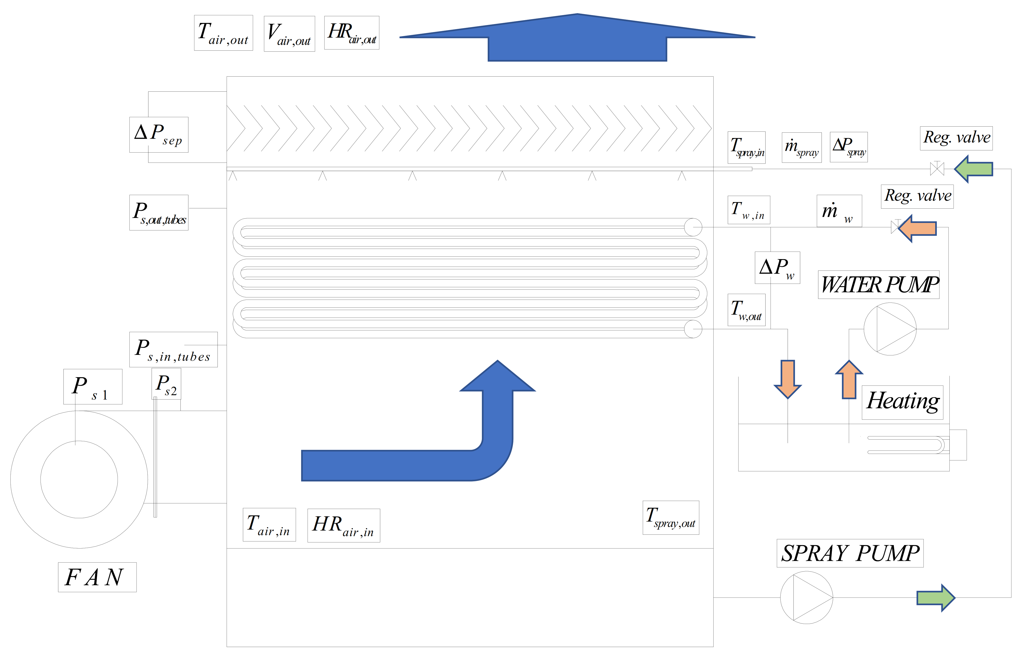
In an indirect closed-circuit cooling tower, there is not direct contact between the air and the fluid being cooled. Unlike the open cooling tower, the indirect cooling tower has three separate fluid flows: one is an internal circuit in which water (or other fluid) is recirculated inside the tube bundle. On the outside of the tubes, sprayed water removes the heat from the inner fluid. Air is drawn around the outer surface of the tubes, providing evaporative cooling. In operation, the heat flows from the internal fluid circuit, through the tube walls of the coils, to the external circuit, and finally the air evaporating the sprayed water to the air stream. A schematic configuration of the cooling tower is presented in Figure 1.

Thermal models of these devices could be considered as sufficiently validated in literature: in Kröger [1], the performance of the models are summarized. The first attempt was proposed by Parker and Treybal [2]. Lately, Mizushima et al. [3,4] developed a simple model with acceptable results. Leidenfrost et al. [5] presented a model similar to that proposed by Parker and demonstrated that acceptable results can only be achieved using iterative techniques.

Although air/water pressure drop across the tube bundle is the main responsible of the final energy consumption in the cooling tower, these previous studies have not paid too much attention to this point. According with Kröger [1], no general correlation valid for all geometries has been presented in literature. The first correlation was proposed by Niitsu et al. [6], and most of the subsequent correlations were presented following the same scheme (Reuter and Anderson [7], Graaff [8]). The main drawback of this type of correlations is that are only applicable to their own geometries.

Due to the lack of reliable air/water pressure drop correlations, the parametric studies found in the literature were obtained by plotting the cooling tower efficiency as a function of the inlet mass flows and temperatures of the three streams involved. The conclusions reached by this type of analysis could lead to a non-optimal design of the cooling tower due to various reasons. Firstly, the temperature approach (the difference between outlet water and the inlet wet bulb temperatures) is the key parameter for determining the cooling tower capacity. Secondly, increasing the three streams by the same percentage of mass flow results in a different effect in the global power consumption of the cooling tower. For these reasons, the ratio between the electrical consumption and the cooling capacity is more representative of the cooling tower performance than the cooling tower efficiency.

The objective of the present study is to predict the air/water pressure drop across tube bundles in annular/mist flow to finally obtain an energy consumption model to perform parametric studies in this type of devices. This energy modeling could allow refrigeration engineers to better select the closed-circuit cooling tower, and in current systems, provide guidelines to improve control techniques and cooling tower performance.

2. Materials and Methods

The experimental equipment established in the present study was developed to investigate the energy consumption of the cooling tower and the associated cooling capacity. Figure 1 shows a schematic of the constructed experimental set up and a diagram of the cooling tower with the main variables. The heat exchanger section consists of a tube bundle of 6 rows and 6 columns in a transversal section of 0.6 m × 0.2 m. The geometrical parameters are $N_{columns}=5$ and $N_{rows}=6$. The tubes are 3/8” (9.52 mm OD, 0.76 mm wall thickness). The experimental set up consists of the cooling tower, the intube water loop, and the spray loop. The heat exchanger section of the cooling tower consists of a centrifugal fan, the tube bundle, drop separator and the nozzles. All variables described in the figure were measured directly except for the water and spray mass flow and the air velocity. The water ${\dot{m}}_w$ and spray mass flow ${\dot{m}}_{spray}$ were obtained by measuring the flowrate and estimating the inlet density of the fluids. The mean air velocity was obtained by direct measurements of the velocity profile at the outlet section and correlating the data with the pressure drop separator following the procedure described in Section 2.1.1.

In the plant, the fan, spray and water pump flow rates and the water loop heating power can be manually or automatically manipulated. The main objective is to control the approach temperature difference (difference between the output water and the inlet wet-bulb temperatures $Approach=T_{w,out}-T_{wb,in}$).

Water and spray flowrate control were performed by manual operation valves, and fine regulation was controlled by TRIACS. These valves produced additional pressure losses, that were not accounted for in the energy consumption model. The fan and pumps energy consumption were obtained by the experimental pressure drop and considering a pump/fan efficiency of 0.3 each. In a real case application, the actual efficiency of the pumps and fan should be considered. In Figure 2 show the constructed experimental setup.

The uncertainty analysis was performed following the method described in the NIST Technical Note 1297 [9]. The measured variables and their uncertainty are presented in

Table 1. Measured variables and their experimental uncertainty.

Variable	Units	Uncertainty
$T_{liquid}$	$\mathrm{°}\mathrm{C}$	$\pm 0.1\mathrm{°}\mathrm{C}$
$T_{air}$	$\mathrm{°}\mathrm{C}$	$\pm 0.2\mathrm{°}\mathrm{C}$
$\Delta P_{air}$	$\mathrm{P}\mathrm{a}$	$\pm 3\%$
$\Delta P_{liquid}$	kPa	$\pm 3\%$
${\dot{V}}_w,{\dot{V}}_{sp}$	$\mathrm{L}\cdot {\mathrm{s}}^{-1}$	$\pm 1\%$
$RH$	$\%$	$\pm 1.5\%$

.

2.1. Data Reduction

Temperature, air humidity and pressure drop measurements were taken on the experimental set up. Air flow measurements were indirectly estimated by correlating data from direct velocity measurements with pitot tubes and the pressure drop at the drop separator. In the case of water and spray, the flow was measured by means of turbine flow meters. A data reduction is needed in the present study to analyze the cooling capacity and energy consumption of the cooling tower.

2.1.1. Air Flow Measurement

Air mass flow in the cooling tower was obtained by correlating the pressure drop in the drop separator and the direct velocity air measurements following a traverse log-Chebycheff method, as specified in ISO 3966:2008 (measurement of fluid flow in closed conduits-velocity area method using pitot static tubes), by taking velocity measurements at 25 points at a constant power consumption. Inlet and outlet temperature and relative humidity air properties were measured with sensors of 0.2 °C and 1.5% HR accuracy, respectively.

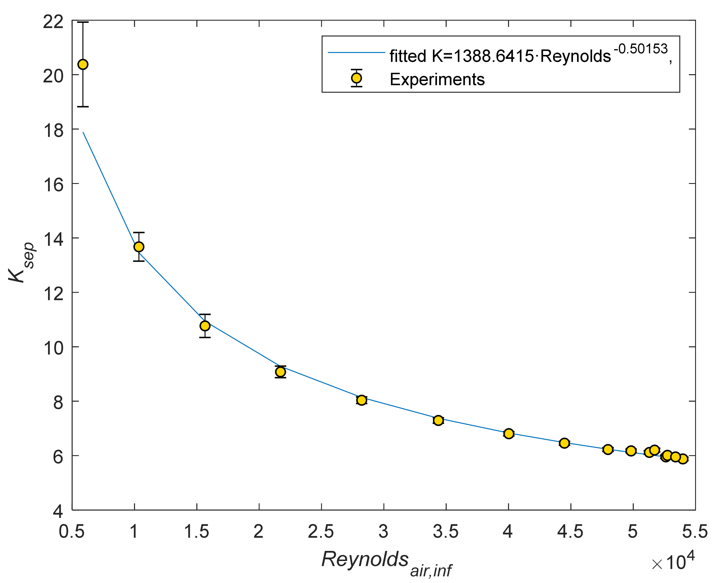
Measuring the air velocity at these 25 points, and regulating the fan velocity, the average velocity was obtained with the method described. The loss coefficient at the drop separator K_separator Equation (1), was calculated using the pressure loss at the separator and the outlet air density data. Calculating the Reynolds number of the air flow, the loss coefficient K_separator was correlated as Equation (2).

$$K_{sep}=\frac{2\cdot \Delta P_{sep}}{{\rho }_{a,out}\cdot V_{\mathit{inf},mean}^2}$$

(1)

$$K_{sep}=1388.6\cdot {\mathit{Re}}_a^{-0.5015}(\mathrm{coefficient}\mathrm{of}\mathrm{determination}{\mathrm{R}}^2=0.9932)$$

(2)

Figure 3 shows the calculated loss coefficient and the fitted data. The separator loss coefficient is correlated within the uncertainty range at Reynolds numbers higher than 5000. Equation (2) is used to estimate the air flow of the cooling tower.

2.1.2. Air Side Heat Balance and Energy Consumption

Once the air flow of the cooling tower has been correlated with the experimental pressure losses at the drop separator, the air velocity in the subsequent paragraphs was calculated by means of Equation (3) with the loss coefficient calculated according to Equation (2).

$$V_a=\sqrt{\frac{2\cdot \Delta P_{sep}}{{\rho }_{a,out}\cdot K_{sep}}}$$

(3)

The air temperature and relative humidity are also used to calculate the enthalpy and absolute humidity of the flow. The dry air mass flow and the dissipated heat were obtained by Equations (4) and (5) respectively.

$${\dot{m}}_{dry,a}=\frac{V_a\cdot A_{section}\cdot {\rho }_{a,out}}{\left({\omega }_{a,out}+1\right)}$$

(4)

$${\dot{Q}}_a={\dot{m}}_{dry,a}\cdot \left(h_{a,out}-h_{a,in}\right)$$

(5)

According to Li et al. [10], the pressure drop in a cooling tower can be differentiated into three terms: pressure losses at the tube bundle, dynamic pressure losses and miscellaneous pressure losses, which include pressure losses at the drop separator.

$$\Delta P_{s,a}=\Delta P_{tubes}+\Delta P_{misc}+\Delta P_{dynamic}$$

(6)

Following the European Commission Regulation No 327/2011 of 30 March 2011, and considering the measurement category A, the efficiency of the fan is calculated from the static pressure difference at the fan, with open inlet and outlet. Considering that the compression effects are negligible, the efficiency is obtained from Equation (7). The electrical consumption of the fan ${\dot{W}}_{elect,fan}$ was calculated considering that ${\eta }_{s,fan}=0.3$.

$${\eta }_{s,fan}=\frac{\Delta P_{s,a}\cdot {\dot{V}}_a}{{\dot{W}}_{elect,fan}}$$

(7)

As the static pressure at the tower inlet is $P_{s1}=-\frac{1}{2}\cdot \rho \cdot V_1^2$, the static pressure difference is obtained by Equation (8):

$$\Delta P_{s,a}=P_{s2}-P_{s1}=P_{s2}+\frac{1}{2}\cdot \rho \cdot V_1^2$$

(8)

The available static pressure difference $\Delta P_{s,available}$ is dissipated in the tube bundle and the different elements of the cooling tower (miscellaneous pressure losses: drop separator, cooling tower structure, nozzles, etc.) The static pressure difference is the fan outlet pressure, minus the kinetic energy at the outlet section of the cooling tower, calculated by Equation (9).

$$\Delta P_{s,available}=P_{s2}=\left(\Delta P_{tube,bundle}+\Delta P_{misc}\right)$$

(9)

Substituting the above equation into Equation (7) gives:

$${\eta }_{s,fan}=\frac{\left(P_{s2}-P_{s1}\right)\cdot {\dot{V}}_{fan}}{{\dot{W}}_{elect,fan}}=\frac{\left[\left(\Delta P_{tube,bundle}+\Delta P_{misc}\right)-P_{s,1}\right]\cdot {\dot{V}}_{fan}}{{\dot{W}}_{elect,fan}}$$

(10)

2.2. Water Side Heat Balance and Energy Consumption

The mass flow of the inlet water side was calculated by means of the measured volumetric flow and the water density.

$${\dot{m}}_w={\dot{V}}_w\cdot {\rho }_{w,in}$$

(11)

The water side volumetric flow was measured with a turbine flowmeter of accuracy $\pm 1\%$. Temperatures at the inlet and outlet were measured with PT100 sensors DIN A. The cooling capacity is calculated in Equation (12).

$${\dot{Q}}_{cooling}={\rho }_{w,in}\cdot {\dot{V}}_{w,in}\cdot C{p}_w\cdot \left(T_{w,in}-T_{w,out}\right)$$

(12)

Water pump energy consumption was calculated using the differential pressure between the inlet and outlet with a sensor of accuracy $\pm 3\%$. The useful energy of the water side is obtained by Equation (13):

$${\dot{W}}_w=\Delta P_w\cdot {\dot{V}}_w$$

(13)

The real energy consumption of the water pump, taking into account pump efficiency, is calculated by Equation (14):

$${\dot{W}}_{w,\exp }=\frac{{\dot{W}}_w}{{\eta }_{pump,w}}$$

(14)

The real energy consumption of the water pump was estimated with a pump efficiency of 0.3.

2.3. Spray Side Heat Balance and Energy Consumption

In modeling the cooling tower, it is assumed that the whole cooling tower is adiabatic, but experimentally this condition is disregarded, so the heat transferred to the water spray is obtained by Equation (15). In Equation (15) the volumetric flow was measured with a turbine flowmeter, and temperatures were measured with PT100 sensors.

$${\dot{Q}}_{sp}={\rho }_{sp,in}\cdot {\dot{V}}_{sp,in}\cdot C{p}_{sp}\cdot \left(T_{sp,in}-T_{sp,out}\right)$$

(15)

The main pressure loss at the spray section is produced at the nozzles. In order to measure this energy loss, a pressure sensor is used and the energy consumption is calculated by Equation (16):

$${\dot{W}}_{sp}=P_{sp}\cdot {\dot{V}}_{sp}$$

(16)

The spray real power consumption is affected by the spray pump efficiency that was not measured. The considered efficiency of the spray pump was 0.3. Thus, the real power consumption of the spray pump is calculated by Equation (17):

$${\dot{W}}_{sp,real}=\frac{{\dot{W}}_{sp}}{{\eta }_{pump,sp}}$$

(17)

2.4. Heat and Mass Transfer Model

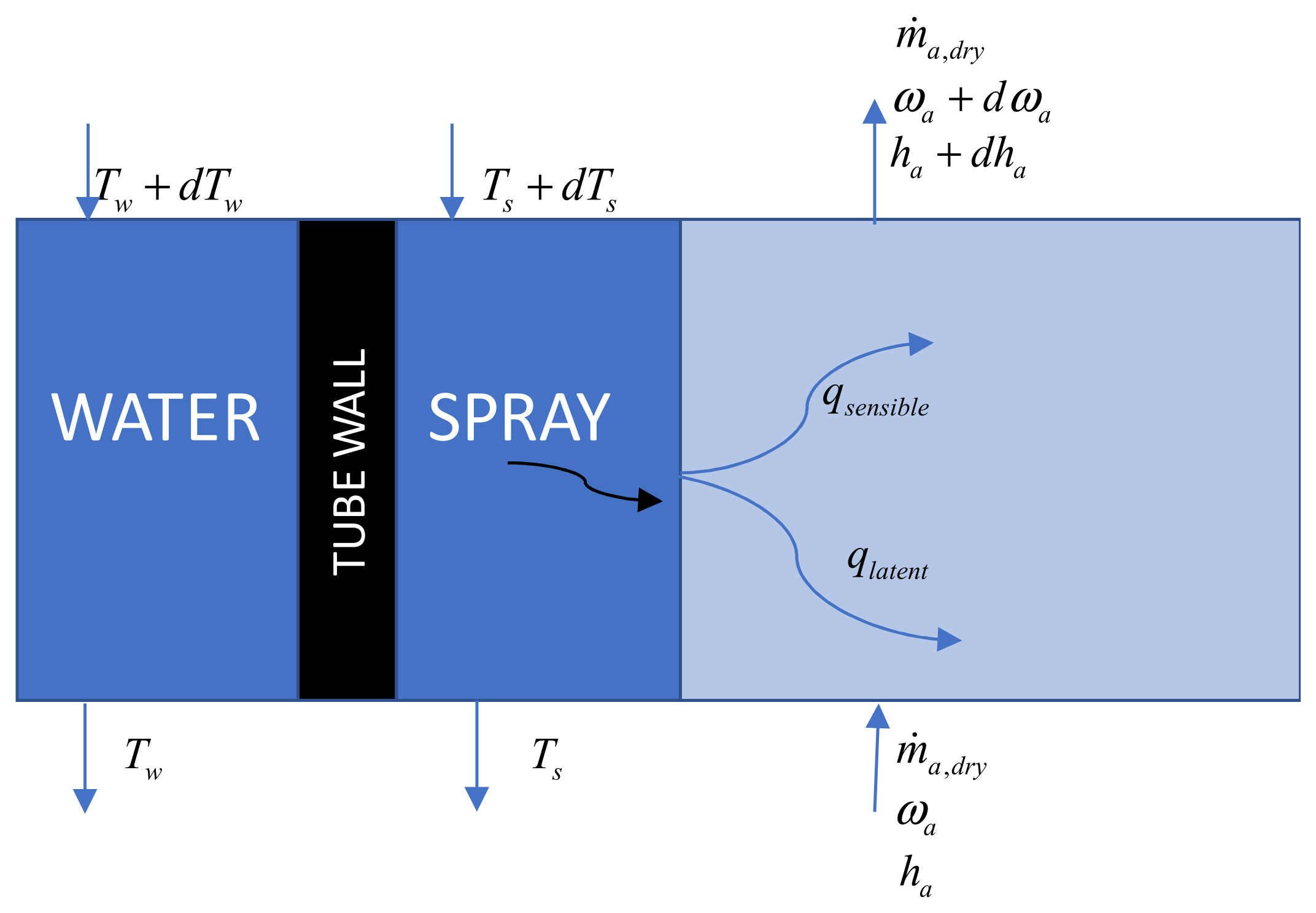
The model of Mizushima [4] has been used by different authors pointing out its simplicity and performance. In this paragraph, a brief description of the model is presented. In a closed-circuit cooling tower, the spray and the air flow in counterflow and the water in crossflow. If it is considered that all the currents flow in the same direction, an analysis of a differential portion of the cooling tower is as shown of Figure 4.

The mass transfer from the spray to the air flow can be obtained by:

$$d{\dot{m}}_a={\alpha }_m\cdot \left({\omega }_i-{\omega }_a\right)\cdot dA$$

(18)

calculating $d{\dot{m}}_a$ by means of the mass flux of dry air, where ${\alpha }_m$ is the mass transfer coefficient for water vapor.

$${\dot{m}}_{dry,a}\cdot d{\omega }_a={\alpha }_m\cdot \left({\omega }_i-{\omega }_a\right)\cdot dA$$

(19)

For simultaneous heat and mass transfer, the heat transfer can be calculated through enthalpy potential. Then the enthalpy variation in the air, in an elementary heat transfer surface $dA$, can be expressed as Equation (20), being $h_i$ the enthalpy at the water/air interface.

$${\dot{m}}_{dry,a}\cdot d{h}_a={\alpha }_m\cdot \left(h_i-h_a\right)\cdot dA$$

(20)

If the spray rate evaporation is neglected at the elementary surface $dA$, the energy balance for the different fluxes can be evaluated as:

$${\dot{m}}_w\cdot C{p}_w\cdot d{T}_w={\dot{m}}_a\cdot d{h}_a-{\dot{m}}_{sp}\cdot C{p}_{sp}\cdot d{T}_{sp}$$

(21)

Additionally, a heat transfer analysis between the water and the spray gives Equation (22):

$$U\cdot \left(T_w-T_i\right)\cdot dA={\dot{m}}_w\cdot C{p}_w\cdot d{T}_w$$

(22)

where $U$ is the local overall heat transfer coefficient between water and film/air interface. This term can be calculated by adding all thermal resistances being $k_{tube}$ the thermal conductivity of the tube.

$$\frac{1}{U}=\frac{1}{{\alpha }_w}\cdot \frac{D_{ext}}{D_{\mathrm{i}nt}}+\frac{D_{ext}}{2\cdot k_{tube}}\cdot \ln \left(\frac{D_{ext}}{D_{\mathrm{int}}}\right)+\frac{1}{{\alpha }_{sp}}$$

(23)

The global heat transfer analysis for the elementary surface $dA$, as it is expressed in Equation (21) could be rewritten by means of Equations (22) and (20), as is shown in Equation (24).

$$U\cdot \left(T_w-T_i\right)\cdot dA={\alpha }_m\cdot \left(h_i-h_{air}\right)\cdot dA-{\dot{m}}_{sp}\cdot C{p}_{sp}\cdot d{T}_{sp}$$

(24)

When calculating tower performance, inlet conditions are known, and outlet conditions are outputs of the model. An interactive procedure is usually applied: water outlet temperature is guessed, which allows the calculation of outlet air properties, and the enthalpy integral of Equation (25). This is known as the Merkel equation.

$$\frac{{\alpha }_m\cdot A}{{\dot{m}}_{air}}={\displaystyle \underset{in}{\overset{out}{\mathrm{\int }}}\frac{d{h}_{air}}{\left(h_i-h_{air}\right)}}$$

(25)

The set of equations of the differential portion of the cooling tower are used in all the models found in the literature. These models differ in the assumed simplifications. The Mizushima and Ito [4] model neglects the interface temperature variation in Equation (25) and considers constant interface conditions throughout the cooling tower. Integration of Equation (25) gives Equation (26).

$$\frac{{\alpha }_m\cdot A}{{\dot{m}}_a}=\ln \left(\frac{h_i-h_{a,in}}{h_i-h_{a,out}}\right)$$

(26)

The integration of Equation (22) and the substitution in Equation (26) leads to:

$$\frac{T_{w,in}-T_i}{T_{w,out}-T}=\frac{h_i-h_{a,in}}{h_i-h_{a,out}}\cdot \exp \left(\frac{U}{{\alpha }_m\cdot C{p}_w}\cdot \frac{{\dot{m}}_a}{{\dot{m}}_w}\right)$$

(27)

which together with the thermodynamic function $h_i=h_i\left(T_i\right)$ form a nonlinear set of equations for calculating $\left(T_i,h_i\right)$.

Integrating Equation (19) in the whole cooling tower, and supposing constant ${\omega }_i$, the equation gives Equation (28):

$$\frac{{\alpha }_m\cdot A}{{\dot{m}}_a}=\ln \left(\frac{{\omega }_i-{\omega }_{a,in}}{{\omega }_i-{\omega }_{a,out}}\right)$$

(28)

The group set of Equations (18)–(28) are used to calculate the outlet conditions of the cooling tower.

2.5. Heat and Mass Transfer Coefficients

Different heat and mass transfer coefficients have been proposed in literature for evaporative cooling devices, and the correlations proposed are summarized in

Table 2. Heat and mass transfer coefficients proposed in literature for evaporative cooling devices.

Author	Air/Water Mass Transfer
Parker and Treybal [2]	${\alpha }_{m,a}=0.064\cdot G_{a,\mathit{max}}^{0.81}$
Niitsu et al. [6]	${\alpha }_{m,a}=0.049\cdot G_{a,\mathit{max}}^{0.9}$
Mizushima and Ito [3]	${\alpha }_{m,a}\cdot a=5.027\times {10}^{-8}\cdot {\mathrm{Re}}_a^{0.8}\cdot {\mathrm{Re}}_s^{0.15}\cdot D_{ext}^{-2.6}$
	Spray Heat Transfer
Parker and Treybal [2]	${\alpha }_{sp}=880\cdot \left(1.39+0.022\cdot T_s\right)\cdot {\left({\mathrm{\Gamma }}_{sp}/D_{ext}\right)}^{0.33}$
Leidenfrost and Korenic [5]	${\alpha }_{sp}=2064\cdot {\left({\mathrm{\Gamma }}_{sp}/D_{ext}\right)}^{0.25}$
Mizushima and Ito [3]	${\alpha }_{sp}=2100\cdot {\left({\mathrm{\Gamma }}_{sp}/D_{ext}\right)}^{0.33}$
	Intube Water Heat Transfer
VDI Heat Atlas [12]	$N{u}_{la\min ar}=4.36$
	$N{u}_{turbulent}=\frac{\left(f/8\right)\cdot \left(\mathrm{Re}-1000\right)\cdot \mathrm{Pr}}{1+12.7\cdot \sqrt{f/8}\cdot \left({\mathrm{Pr}}^{2/3}-1\right)}$
	$\begin{array}{l}N{u}_{transition}=tr\cdot N{u}_{turb(\mathrm{Re}=4000)}+\left(1-tr\right)\cdot N{u}_{lam(\mathrm{Re}=2300)}\\ tr=\frac{\mathrm{Re}-2300}{4000-2300}\end{array}$

. Discussion of this equations were performed by Facão and Oliveira [11], Kröger [1], among others. The experimental conditions of this work cannot evaluate separately the spray and the air/water heat and mass transfer coefficients. As a result, the spray and air/water correlations were selected by the ability to predict the experimental cooling capacity.

2.6. Pressure Drop and Energy Consumption

The energy consumption model has been developed as simple as possible, giving the opportunity to be implemented easily in other geometries from different literature sources. The main obstacle to develop a reliable energy consumption model is in the pressure losses of the air/water stream. Uncertainties exist in the minor losses across the entire section and in the pressure drop at the tube bundle.

2.6.1. Air/Water Phase Energy Consumption

The ${\dot{W}}_{elect,fan}$ is needed to compensate the $\Delta P_{tubes}$, $\Delta P_{misc}$ and $\Delta P_{dynamic}$ pressure drop by the equation:

$${\dot{W}}_{elect,fan}=\frac{\left(\Delta P_{tubes}+\Delta P_{misc}+\Delta P_{dynamic}\right)\cdot {\dot{V}}_a}{{\eta }_{s,fan}}$$

(29)

Being $\Delta P_{total}=\left(\Delta P_{tubes}+\Delta P_{misc}+\Delta P_{dynamic}\right)$. Li and Priddy [10,11] offered an estimation of the $\Delta P_{misc}$ and $\Delta P_{dynamic}$ as:

$$\Delta P_{misc,calc}=6.5\cdot \rho \cdot \frac{V_{out}^2}{2}$$

(30)

$$\Delta P_{dynamic,calc}=\frac{2}{3}\cdot \Delta P_{Total}$$

(31)

As a result, the total pressure drop is calculated as:

$$\Delta P_{total}=3\cdot \left(\Delta P_{tubes}+\Delta P_{misc}\right)$$

(32)

The term $\Delta P_{tubes}$ needs some discussion. According to Ribatski and Jacobi [13,14]. No general correlation is useful for all the possible gas and liquid phase flow combinations in pressure drop across tube bundles in two phase flow.

In evaporative cooling devices, the flow pattern identified is characterized by a continuum liquid film around tubes with the gas phase flowing in the core of the tube bundle. If higher liquid mass flux is added, the tube bundle becomes flooded, increasing the pressure drop and in detrimental of the heat and mass transfer processes. The description of the flow pattern coincides with that annular flow (Xu et al. [14]) or mist flow (Finlay and McMillan [15]).

Niitsu et al. [6] were the first authors that analyzed the pressure drop across tube bundles in air/water mixtures across tube bundles in evaporative coolers. The correlation proposed was of the type:

$$\frac{\Delta P_{TP}}{Z}=a\cdot G_{air}^b\cdot {\left(\frac{\mathrm{\Gamma }}{D_{ext}}\right)}^c$$

(33)

where the constants depend on the geometry of the cooling tower. Most of the studies that investigated the pressure drop in evaporative cooling devices, modified the constants of the equation to adequate to their experiments data. Examples of these equations can be found in [7,16,17].

In two phase flow across tube bundles Ishihara et al. [18], proposed a Martinelli type equation, with a constant value $C=8$

$${\phi }_l^2=\frac{\Delta P_{TP}^F}{\Delta P_l^F}=1+\frac{C}{X}\cdot +\frac{1}{X_{}^2}\hspace{1em}\hspace{1em}if{\mathrm{Re}}_l>2000$$

(34)

$${\phi }_g^2=\frac{\Delta P_{TP}^F}{\Delta P_g^F}=1+C\cdot X\cdot +X_{}^2\hspace{1em}\hspace{1em}if{\mathrm{Re}}_l<2000$$

(35)

where the Martinelli parameter is the square root of the ratio between liquid and gas phases pressure drop.

$$X=\sqrt{\frac{\Delta P_l}{\Delta P_g}}$$

(36)

Ishihara proposed the simplified equation considering that the liquid and gas phases are turbulent.

$$X_{tt}={\left(\frac{1-x}{x}\right)}^{0.9}\cdot {\left(\frac{{\rho }_G}{{\rho }_L}\right)}^{0.5}\cdot {\left(\frac{{\mu }_L}{{\mu }_G}\right)}^{0.1}$$

(37)

In the correlation proposed by Ishihara et al. [18] a single phase pressure drop correlation is needed to calculate the gas phase pressure drop of Equations (34) and (35). In literature, the Gaddis [19], and Zukauskas [20] correlations for single phase pressure drop calculations were recommended.

General pressure drop correlations are preferred instead of adjusting the constants of the correlations of Niitsu et al. [6], as the constants proposed for the correlation of Niitsu depend on geometry.

2.6.2. Water and Spray Pressure Drop

The water pressure drop was calculated supposing that friction losses at the heat exchanger are dominant in the intube water, and the Colebrook equation was used for the turbulent region above Re = 4000. Between the laminar and turbulent region, a linear interpolation between the two regimes was considered. The minor losses were accounted to be 20% of the frictional pressure drop in the tube bank. As a result, the energy calculated is obtained by means of Equation (38):

$${\dot{W}}_{water,calc}=\frac{\left(\Delta P_{w,friction}+0.2\cdot \Delta P_{w,friction}\right)\cdot {\dot{V}}_w}{{\eta }_{w,pump}}$$

(38)

Spray pressure drop is controlled mainly by the minimum operating pressure of the nozzles. It was experimentally observed that the pressure should be higher than 100 kPa. Thus, the calculated spray energy consumption is obtained as.

$${\dot{W}}_{s,calc}=\frac{100kPa\cdot {\dot{V}}_s}{{\eta }_{s,pump}}$$

(39)

3. Results and Discussion

A series of experiments have been carried out to validate and study the heat transfer and energy consumption model of the cooling tower.

Table 3. Experimental range of the main variables involved.

Variable	Range	Variable	Range
$T_{wb,in}\left(\mathrm{°}\mathrm{C}\right)$	13–21	${\mathrm{Re}}_{w,in}$	617–8030
$T_{w,in}\left(\mathrm{°}\mathrm{C}\right)$	16–31	${\dot{m}}_s\left(\mathrm{liters}\times {\mathrm{h}}^{-1}\right)$	50–80
$H{R}_{out}\left(\%\right)$	76–97	$V_{a,\mathit{inf}}\left(\mathrm{m}\times {\mathrm{s}}^{-1}\right)$	0.43–2.7

represents the studied ranges of the inlet variables. The experimental and calculated results have been obtained following the procedures described in previous paragraphs. As a first step of the analysis, a comparison between predicted and experimental results was performed in order to validate the cooling tower heat transfer model. The best performance of the model is obtained when using the correlations of Parker and Treybal [2] for the air mass transfer coefficient and the spray heat transfer coefficient. It should be noted that Mizushima et al. [4] correlations give also good results.

Table 4. Mean error and percentage of data points within the 20% margin error for the different correlations.

Air mass Transfer	Spray Heat Transfer	Mean Error	Percentage of Data within 20%
Parker and Treybal [2]	Mizushima and Ito [4]	−1.38	84.13
	Parker and Treybal [2]	0.03	84.13
	Leidenfrost and Korenic [5]	7.91	73.02
Niitsu et al. [6]	Mizushima and Ito [4]	−2.37	81.75
	Parker and Treybal [2]	−0.95	83.33
	Leidenfrost and Korenic [5]	7.08	74.60
Mizushima and Ito [4]	Mizushima and Ito [4]	2.03	81.75
	Parker and Treybal [2]	3.35	83.33
	Leidenfrost and Korenic [5]	10.73	69.84

shows the performance of the model with the correlations considered, under the experimental conditions specified in Table 3.

Figure 5 shows the calculated cooling capacity vs the experimental cooling capacity of the cooling tower with the spray and mass transfer coefficient calculated by Parker and Treybal [2]. It can be observed that larger deviations are obtained at lower cooling capacities. These discrepancies are produced when the Reynolds number of the intube water is in the transition from turbulent to laminar region.

3.1. Air/Water Pressure Drop-in Two-Phase Flow

Air/water fan energy consumption modeling requires some extra work. Pressure drop in the air/water biphasic flow comprises the pressure drop in the tube bundle, the dynamic pressure drops, and the miscellaneous pressure drops $\Delta P_{misc}$, produced in the drop separator and in other elements of the cooling tower. For the sake of simplicity of the model, the pressure loss at the drop separator was equal to the miscellaneous $\Delta P_{misc}=\Delta P_{separator}$, as $\Delta P_{separator}$ that is the main source of the miscellaneous pressure drop. More complex models could be elaborated following the advices found in Kröger [1].

Figure 6 shows the pressure drop at the drop separator $\Delta P_{separator}$, and the predicted $\Delta P_{misc}$ pressure drop following the recommendation of Li and Priddy [10]. As it can be seen, the miscellaneous pressure drop calculated by a constant like the suggested by the authors could yield to errors in modeling at low velocities.

3.1.1. Air/Water Pressure Drop Across the Tube Bundle

The correlation of Ishihara et al. [18] was used to calculate the pressure drop across the tube bundle. This correlation is preferred for numerical optimization purposes, if their predictions are reasonable, instead of the proposed by Niitsu et al. [6], since they only depends on a constant.

Ishihara et al. [18] correlation calculates the two-phase multiplier factor as:

$${\phi }_{L,calc}^2=\frac{\Delta P_{TP,calc}}{\Delta P_L}=1+\frac{C}{X_{tt}}+\frac{1}{X_{tt}^2}$$

(40)

The authors used the Martinelli parameter considering that the phases are turbulent as.

$$X_{tt}={\left(\frac{1-x}{x}\right)}^{0.9}\cdot {\left(\frac{{\rho }_G}{{\rho }_L}\right)}^{0.5}\cdot {\left(\frac{{\mu }_L}{{\mu }_G}\right)}^{0.1}$$

(41)

In Equation (40) $\Delta P_l^{}$ is the liquid phase pressure drop of the liquid phase flowing alone. Experiments with air in single phase flow were performed to obtain the single-phase pressure drop equation. The experimental friction factor was obtained as:

$$f=\frac{\rho \cdot \Delta P_f}{2\cdot N\cdot G_{\mathit{max}}^2}$$

(42)

Finally, the friction factor was correlated as:

$$f=\frac{1.289}{{\mathrm{Re}}_{D,\max }^{0.2683}}for400<{\mathrm{Re}}_{D,\max }^{}<2400$$

(43)

The calculated pressure drop by the Ishihara correlations was compared with the experimental data obtained in the cooling tower. In our experiments, the experimental two-phase multiplier factor was obtained as:

$${\phi }_{L,\exp }^2=\frac{\Delta P_{TP,\exp }}{\Delta P_L}$$

(44)

Figure 7 shows the two phase multiplier factor, calculated by Equation (44), as a function of the Martinelli parameter, calculated as in Equation (44), and a comparison with the Ishihara correlation defined for the liquid phase ${\phi }_l^2$. As it can be observed, the calculated two-phase multiplier tends to overpredict the experimental data. Discrepancies could be explained, mainly because the Ishihara correlation assumes that the friction factor ratio between liquid and gas phases are near the unity. This represents a problem when the calculated liquid Reynolds number is lower than 2000, as the friction factor in laminar region increases considerably.

To overcome this problem, Ishihara recommended the use ${\varphi }_g^2$ instead of the ${\varphi }_l^2$ when the ${\mathrm{Re}}_l<2000$, but this procedure yield to discontinuities if a numerical study is purposed. Figure 8 represents the experimental two-phase multiplier factor as a function of the Martinelli parameter calculated as ${\rm X}=\sqrt{\Delta P_L/\Delta P_G}$. As it can be observed, the experimental data is well correlated taking this consideration into account. The results suggests than in evaporative cooling devices, characterized by low gas and liquid mass fluxes the Ishihara correlation could predict the experimental data reasonably. The constant $C=8$ should be maintained constant until more experimental data (with different mass fluxes and geometries) were available.

3.1.2. Air/Water Miscellaneous Pressure Drop

Following the procedure proposed by Li and Priddy [10], the dynamic pressure losses are estimated as $2/3\cdot \Delta P_{total}$, so the total pressure drop was calculated as:

$$\Delta P_{total,calc}=3\cdot \left(\Delta P_{tubes}+\Delta P_{separator}\right)$$

(45)

Figure 9 shows the total pressure drop measured as $\Delta P_{TOTAL,\exp }=P_{s,2}-P_{s,1}$ in comparison with the predictions of the equation, and also the best adjustment of data using K = 3.31. The differences between the recommendation of Li and Priddy [10] and the experimental data could be explained by the neglection of some of the miscellaneous pressure drops.

Pressure drop across tube bundles in evaporative cooling devices are characterized by low liquid mass flows. The assumption that the liquid and gas phases flow in turbulent regime causes incoherencies in the calculated pressure drop using the Ishihara correlation. The original definition of the Martinelli parameter $\mathrm{X}=\sqrt{\Delta P_L/\Delta P_G}$ for these conditions give better predictions.

3.2. Water Flow Rate Influence on the Energy Consumption to Cooling Capacity Ratio

According to Zalewski et al. [21], the energy consumption of the water circuit is negligible, but the heat transfer coefficient may influence the cooling tower capacity. A set of experiments was performed to investigate the influence of the water Reynolds number on the cooling capacity of the tower.

Figure 10 shows the experimental water temperature difference obtained between inlet and outlet for different water Reynolds numbers while maintaining a constant approach temperature, air velocity and spray flow rate. The trend of the model agrees with the experimental data, although the deviations are larger for Reynolds numbers between 1000 and 2500, probably due to a different flow distribution through the tubes.

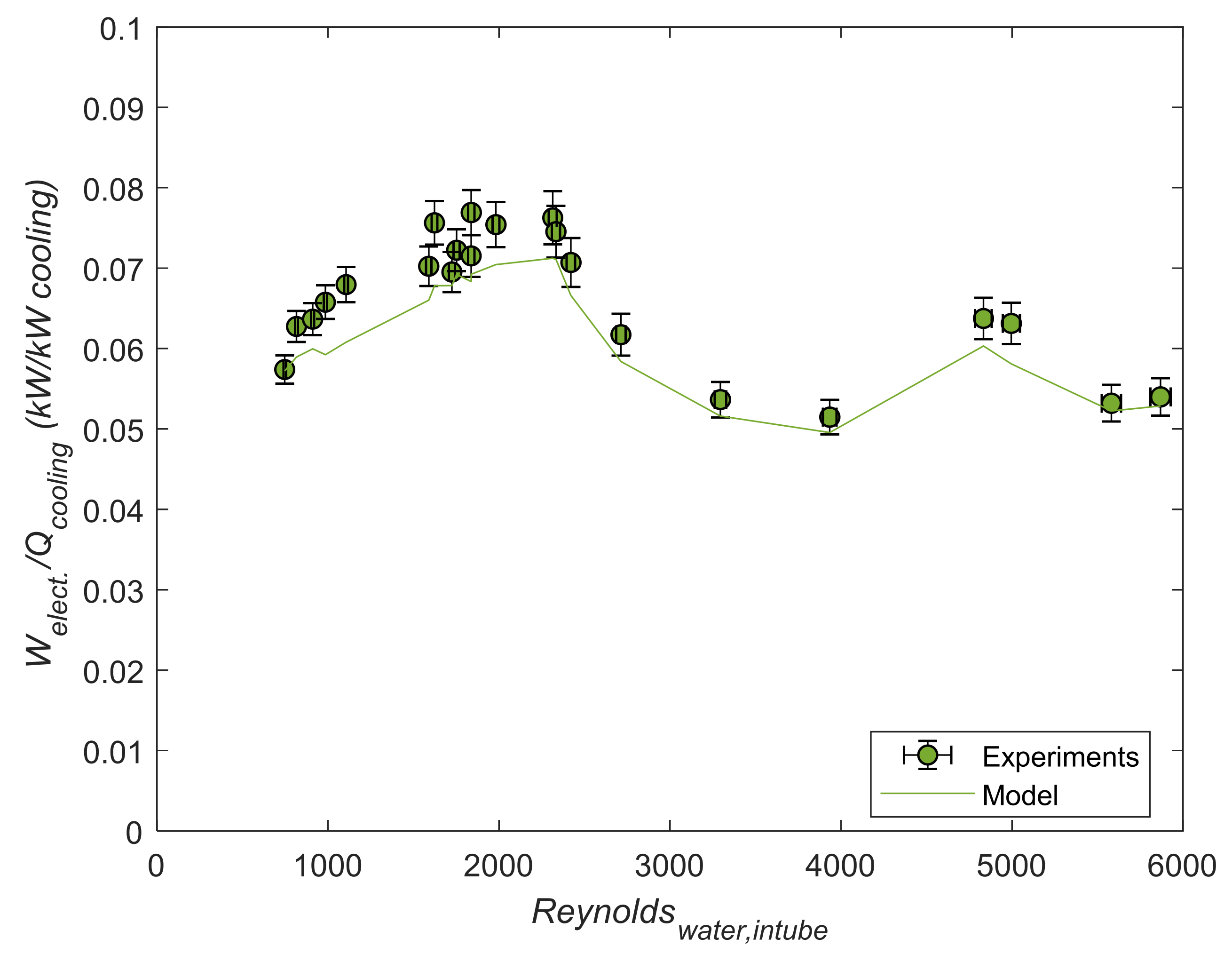
Figure 11 shows the cooling tower energy consumption per kW dissipated. For the performed experiments, the lowest energy ratio is obtained at a Reynolds number of 4000. In the laminar region the heat transfer coefficient is expected to be constant. In this region, increasing the mass flow rate reduces the mean temperature gradient between the water and wet bulb temperature as shown in Figure 10.

Reaching the transition region, the energy consumption increases with the pressure drop, although the cooling capacity also increases due to the heat transfer coefficient. This tendency reaches a minimum energy consumption per cooling capacity, when the pump energy consumption exceeds the heat dissipated.

A further increase in water pump energy penalizes the energy consumption. These results are in accordance with that of Zalewski et al. [21]. The authors stated that modifying the water flow does not imply an increase in the cooling capacity.

The intube water Reynolds number influences the cooling capacity of the cooling tower at lower Reynolds numbers of 4000. The experimental results shows that turbulence has impact on the cooling capacity of the cooling tower. A further increase of the Reynolds number increases the energy consumption of the cooling tower, but with little effect on the cooling capacity.

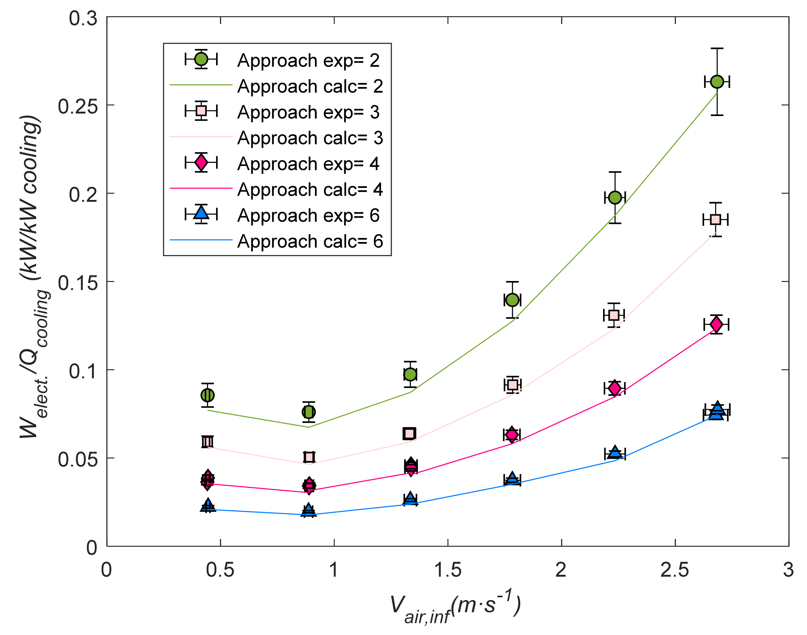
3.3. Cooling Tower Energy to Cooling Capacity Ratio as a Function of the Air Velocity and Approach Temperature

As it has been mentioned before, once the geometrical parameters are established, the approach temperature difference and the air flow are the key parameters for determining the cooling tower capacity. Figure 12 shows the cooling tower energy ratio, as a function of the air velocity and approach temperature. Experimental data was obtained for a constant water Reynolds number of 5000 and a mean spray flow of 80 kg·h⁻¹. Figure 12 also shows the same trend as the experimental data. As was expected, the energy ratio increases with the approach temperature. For a constant approach temperature, the lowest energy consumption per kW dissipated is obtained at air velocities near 1 m·s⁻¹.

For the chosen geometrical parameters, it was also noted that approach temperatures higher than 6 °C yield the same energy ratio. Additionally, the energy ratio is not seriously penalized by increasing the air flow. Under these conditions, regulating the air flow can be beneficial in terms of performance.

4. Conclusions

Cooling tower experiments and an energy consumption modeling have been performed in this study. Energy consumption, pressure drops, and cooling capacity have been analyzed. The model was validated by experimental data, and it can predict the cooling capacity of the cooling tower with an average error of 3%, and with 90% of the data within $\pm 15\%$ accuracy.

The literature review showed that no general pressure drop correlation in air/water two-phase flow across tube bundles was used successfully in evaporative cooling devices. The use of a reliable correlation opens the possibility to perform parametric studies in different geometries than the studied. The correlation proposed by Ishihara et al. [17] using the Martinelli parameter considering that the two phases are turbulent underpredict the data. In the experiments, the calculated Reynolds numbers of gas and liquid phases are laminar, suggesting that the assumption of the Martinelli number is not feasible for these experiments. The original definition of the Martinelli parameter $X=\sqrt{\Delta P_L/\Delta P_G}$ was used successfully predicting two phase pressured drop for the observed annular/mist flow on the tube bundle. Minor losses at the cooling tower are mainly controlled by the drop separator. Li and Pryddy [10] suggested a loss coefficient of 6.5 for the miscellaneous pressure drop, giving underpredictions at low air velocities.

The model proposed has limited use of empirical constants which make the model valid for other configurations. The model shows that the trends are in accordance with the experimental data under the different operating parameters investigated. Water pump, spray pump, and fan efficiencies are needed to develop a model of a real cooling tower.

According to the experimental data and modeling, the water flowrate has no effect on the cooling capacity in the turbulent region. The recommended Reynolds number is 4000, near the transition region and higher Reynolds numbers only increase the power consumption.

The approach temperature is the key parameter to reduce the ratio of energy consumption to kW dissipated. For approach temperatures lower than 3 °C, the energy ratio increases rapidly with the air velocity and at approach temperatures higher than 6 °C the energy ratio is not seriously affected. The energy consumption model provides better insight of a cooling tower and may help designers to develop more efficient systems.

References

- Krög̲er, D.G. Air-Cooled Heat Exchangers and Cooling Towers: Vol. 2: Thermal-Flower Performance Evaluation and Design; PennWell Corporation: Tulsa, OK, USA, 2004; ISBN 9781593700195. [Google Scholar]
- Parker, R.O.; Treybal, R.E. The heat, mass transfer characteristics of evaporative coolers. AIChE Chem. Eng. Prog. Symp. Serires 1961, 57, 138–149. [Google Scholar]
- Mizushima, T.; Ito, R.; Miyashita, H. Experimental study of an evaporative cooler. Int. Chem. Eng. 1967, 7, 727–732. [Google Scholar]
- Mizushima, T.; Ito, R.; Miyashita, H. Characteristics and methods of thermal design of evaporative coolers. Int. Chem. Eng. 1968, 8, 532–538. [Google Scholar]
- Leidenfrost, W.; Korenic, B. Evaporative Cooling and Heat Transfer Augmentation Related to Reduced Condenser Temperatures. Heat Transf. Eng. 1982, 3, 38–59. [Google Scholar] [CrossRef]
- Niitsu, Y.; Naito, K.; Anzai, T. Studies on characteristics and design procedure of evaporative coolers. J. SHASE Japan 1967, 41, 12. [Google Scholar]
- Reuter, H.; Anderson, N. Performance evaluation of a bare tube air-cooled heat exchanger bundle in wet and dry mode. Appl. Therm. Eng. 2016, 105, 1030–1040. [Google Scholar] [CrossRef]
- Graaff, A.H. Performance Evaluation of a Hybrid (Dry/Wet) Cooling System; Stellenbosch University: Stellenbosch, South Africa, 2017. [Google Scholar]
- Taylor, B.N.; Kuyatt, C.E. Guidelines for Evaluating and Expressing the Uncertainty of NIST Measurement Results; National Institute of Standards and Technology: Gaithersburg, MD, USA, 1994. [Google Scholar]
- Li, K.W.; Priddy, A.P. Power Plant. System Design; John Wiley: Hoboken, NJ, USA, 1985. [Google Scholar]
- Facão, J.; Oliveira, A. Heat and mass transfer correlations for the design of small indirect contact cooling towers. Appl. Therm. Eng. 2004, 24, 1969–1978. [Google Scholar] [CrossRef]
- Wagner, W. VDI Heat Atlas; Springer: Berlin, Germany, 2010; ISBN 9783540778769. [Google Scholar]
- Ribatski, G.; Jacobi, A.M. Falling-film evaporation on horizontal tubes—A critical review. Int. J. Refrig. 2005, 28, 635–653. [Google Scholar] [CrossRef]
- Xu, G.P.; Tou, K.W.; Tso, C.P. Two-Phase Void Fraction and Pressure Drop in Horizontal Crossflow Across a Tube Bundle. J. Fluids Eng. 1998, 120, 140–145. [Google Scholar] [CrossRef]
- Finlay, I.C.; McMillan, T. Pressure loss during air/water mist flow across a staggered bank of tubes. Int. J. Multiph. Flow 1974. [Google Scholar] [CrossRef]
- Tezuka, S.; Kasai, S.; Nakamura, T. Performance of an evaporative cooler. Heat Transf. Res. 1976, 6, 1–18. [Google Scholar]
- Heyns, J.A.; Kröger, D.G. Experimental investigation into the thermal-flow performance characteristics of an evaporative cooler. Appl. Therm. Eng. 2010, 30, 492–498. [Google Scholar] [CrossRef]
- Ishihara, K.; Palen, J.W.; Taborek, J. Critical Review of Correlations for Predicting Two-Phase Flow Pressure Drop across Tube Banks. Heat Transf. Eng. 1980, 1, 23–32. [Google Scholar] [CrossRef]
- Gaddis, E.S. Pressure drop of tube bundles in cross flow. In VDI Heat Atlas; Springer: Berlin, Germany, 2000; ISBN 9783540778769. [Google Scholar]
- Žukauskas, A. Advances in Heat Transfer; Elsevier: Amsterdam, The Netherlands, 1972; Volume 8, ISBN 9780120200085. [Google Scholar]
- Zalewski, W.; Niezgoda-Żelasko, B.; Litwin, M. Optimization of evaporative fluid coolers. Int. J. Refrig. 2000, 23, 553–565. [Google Scholar] [CrossRef]
Figure 1.
Closed circuit cooling tower and the fluid streams involved.
Figure 2.
Experimental setup.
Figure 3.
Calculated loss coefficient for different Reynolds numbers and fitted data.
Figure 4.
Differential analysis of the cooling tower.
Figure 5.
Predicted cooling capacity vs. the experimental cooling capacity.
Figure 6.
Pressure drop at the drop separator in comparison with the calculated by Equation (30).
Figure 7.
Two phase multiplier factor as a function of the Martinelli parameter considering the two phases as turbulent.
Figure 8.
Two phase multiplier factor as a function of the Martinelli parameter considering , and prediction of the Ishihara correlation.
Figure 9.
Total pressure drop at the air/water section of the cooling tower an predictions obtained by Equation (45).
Figure 10.
Water temperature difference between inlet and outlet for different Reynolds numbers. Air flow rate and spray flow rate constant. The approach temperature was maintained at the constant temperature of 4 °C.
Figure 11.
Experimental energy to cooling capacity ratio for different water Reynolds numbers at a constant air and spray flow rate, and the constant approach temperature of 4 °C.
Figure 12.
Experimental energy to cooling capacity ratio for different approach temperatures and air velocities. Data obtained at a constant water Reynolds number of 5000, and spray flow 80 kg·h−1.