Abstract
We previously proposed that the optical centroid efficiency (OCE) might be a preferred figure-of-merit to the enclosed energy of a rectangular pixel (EOD) for an instrument subject to unpredictable environmental jitter and alignment conditions. Here we follow the same symbols for the corresponding quantities, particularly the width of the pixel as being equal to 2d. Here we analyze the performance of the OCE vs. the EOD for the three Seidel primary aberrations of an optical component: spherical, coma, and astigmatism, plus defocus. We show that the OCE has an approximate U-shape when graphed against the EOD, for the aberrations ranging from 0 to 1.25λ. We conclude that for pixels larger than 2d = 3λF/#, a small pixel will feature better performance when expecting jitter, misalignment, and other environmental and unpredictable conditions. When evaluating the performance of low-aberration instruments in dynamic and unpredictable environments, the choice of the lager pixel 2d = 7λF/# might be advantageous. Its selection will result in the deterioration of image resolution.
1. Introduction
In a modern sensor, the perturbations of figure-of-merit include inherent design aberrations, manufacturing uncertainties and misalignment, and some unrealized environment impacts, including jitter, and other unpredictable opto-mechatronics conditions. In the previous work, the correlation between the detector pixel sizes as well as the central obscuration of the optical sensor and the OCE has been presented in detail [1]. In order to explore more characteristics of the OCE, in this follow-up study of previous work some of the most prominent aberrations in a sensor are included. Please note that when dealing with pixel size, we do not study sampling, which is a different phenomenon [2,3]. Similarly, we do not consider any image processing and enhancement that might facilitate or improve the acquisition of the information content in the image [4,5,6,7].
2. Aberration in an Optical Sensor
Descriptions of optical aberrations may be founded in many optical textbooks [8,9,10,11]. In general, the five Seidel sum, “spherical, coma, astigmatism, Petzval curvature, distortion and defocus”, are an excellent representation. In this work we focus on the evaluation of OCE caused by each of the three typical aberrations (spherical, coma, and astigmatism) and defocus in Section 3, Section 4, Section 5 and Section 6. The image is located at the best focus. Also, all the terminologies employed in the following sections are identical to the previous work.
We investigate the relationship between the OCE and the EOD. The prf is based on the chief ray selection. The centroid is calculated after statistical averaging. All aberration studies are performed for two different pixel sizes, 2d = 3λF/# and 2d = 7λF/#, where the linear detector pixel dimension is 2d. This choice corresponds to a relatively small and relatively large pixel size in comparison to the diameter of the Airy disc. The former is a bit larger than the Airy disc diameter, while the latter is somewhat smaller than three Airy discs. In Code V, the aberration represented with an appropriate coefficient in Zernike polynomials for each aberration is added at the entrance pupil of our optical model.
3. Spherical Aberration Studies, a40ρ4
3.1. Spherical for Small Pixel Values, 2d = 3λF/#
We investigate the relationship between the OCE and the EOD for the increase in spherical aberration from a40 = 0 to a40 = 1.25λ. The results for small pixel size 2d = 3λF/# are presented as the OCE vs. EOD graph in Figure 1. The EOD values are arranged in the ascending order from about 0.3 to about 0.9, corresponding to the decrease in the amount of the spherical aberration from bottom left (a40 = 1.25λ) to top right (a40 = 0) of the graph. As the amount of spherical aberration increases, the energy in the central peak of the psf-s is pushed out symmetrically to the side lobes in the radial direction. The addition of spherical aberration results in the reduction of the EOD.
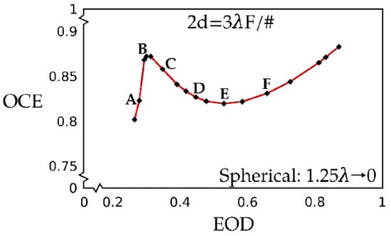
Figure 1.
OCE vs. EOD for a lens with the spherical aberration (ρ4-term) for a detector pixel size of 2d = 3λF/#. The amount of spherical aberration decreases from the lower left corner with the value of a40 = 1.25λ along the curve to the upper right corner with a40 = 0.
When there is no aberration, the OCE achieves a value of 0.88 for the maximum energy on the detector enclosed by the square pixel, and an EOD value of 0.88 for pixel size 2d = 3λF/#. The OCE first smoothly decreases with increasing amount of aberration, arriving at a local minimum of 0.82 for the EOD of 0.58. Then OCE climbs to a sharp peak, nearly equal to the case of zero (0) aberration around the aberration value a40 = 1λ. When the aberration further increases, the lowest value is achieved for the OCE, equal to 0.80 for an EOD of 0.25.
Here we note that the OCE is proportional to the EOD for about half of the EOD interval and inversely proportional over the other half. We may simply observe that they are not correlated. We use the description that two quantities are correlated when they either increase or decrease under similar circumstances. Two quantities are not correlated when their changes occur under different circumstances.
For a small pixel size of 2d = 3λF/#, the OCE first rapidly increases with increasing values of EOD, reaching a maximum of 0.872 when the EOD is equal to 0.31. The low value of the EOD is caused by the fact that the energy moves from the central spot to the higher-order rings for a high amount of aspherical aberration. When the optical axis relative to the pixel position moves around in the OCE determination, the position of the image centroid has no deteriorating consequence because the amount of energy is about the same all over the pixel surface. The OCE value is relatively high because the normalization with the EOD is included in its definition.
The OCE peak around 1λ aberration is followed by a sharp decrease in the OCE values when the EOD is further increased, until a broad minimum is attained at EOD = 0.53, with the still-high value of 0.82 for the OCE. In this region, the amount of spherical aberration has decreased, so the spot is becoming better defined, resulting in increased energy collection over the pixel surface. A more compact spot results in smaller average energy on detector for a displaced pixel center and increased energy on detector for the centered image. Both effects combine to decrease the OCE for small pixel size 2d = 3λF/#. Here, the displacement of the spot position over the pixel area is very sensitive. Only with decreasing aberration values are the OCE and the EOD correlated as expected when the spot over the pixel surface becomes compact under conditions of no or a small amount of aberration.
Figure 2 presents cross-sections of the instrument point response function prf as a function of a radial coordinate, normalized to pixel size for the points labeled in Figure 1, that is, A, B, C, D, E, and F.
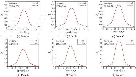
Figure 2.
The instrument point response function prf corresponding to selected points in Figure 1 as a function of two orthogonal directions, x and y, or rows and columns, for the case of spherical aberration. The amount of aberration decreases from about a40 = 1λ to a40 = 0.5λ, going from (a–f). With the decrease in the aberration, the power in the image becomes increasingly more centralized. The figures are arranged in order of increasing energy on the detector, which corresponds to a decreasing amount of aberration. The graphs in the first row correspond to the peak in the OCE vs. EOD graph in Figure 1, while those in the second row correspond to the valley. The common features of the prf-graphs for the peak are a decreased peak value, an increased amount of the compact support, and the fact that the images carry a significant amount of aberration. The valley is characterized by a relatively high peak value, the absence of compact support, and a decreased amount of aberration. Due to the symmetry of the problem, the red line overlaps over the blue line.
First, we study the three points near the narrow and sharp peak, that is, Points A, B, and C. The corresponding prf-graphs are plotted in Figure 2a–c. At first glance, these three graphs, lined in the first row, appear to be quite like the ones in the second row.
The most important difference to note is the relatively large difference in the prf-values between the center (0) and edge of the detector pixel (0.5). Point B has the highest difference between these two values; therefore, it is located near the local peak for the lower EOD regime. The prf-value at the pixel center (0.) is equal to 0.30. The value of the prf at the pixel edge (0.5) is 0.17. The difference in the prf-values at the center and the edge of the detector pixel is 0.13, for a small pixel value of 2d =3λF/#.
The point A is located at nearly the lowest value of the EOD, 0.279. The prf-value at the pixel center is equal to 0.279. The value of the prf at the pixel edge (0.5) is 0.22. The difference in the prf-values at the center and the edge of the detector pixel is 0.123, a value smaller than that at Point B; therefore, the OCE is also smaller for Point A than for Point B. Point C is located at the value of the EOD higher than that for the highest point (B), at 0.345. The prf-value at the pixel center is equal to 0.345. The value of the prf at the pixel edge (0.5) is 0.24. The difference in the prf-values at the center and the edge of the detector pixel is 0.105, a value smaller than that of Point B; therefore, the OCE is also smaller for Point C than for Point B.
Next, we investigate the OCE vs. EOD relationship around the minimum. Figure 2d–f display the three prf plots for Points D, E, and F around the minimum. Point F, featured on Figure 2f, exhibits a peak of the prf graph, that is, the EOD, of 0.66. We see that the value of the prf at the pixel edge (0.5) is 0.36. The difference in the prf at the center, or the EOD, and that the edge of the pixel (0.5) is 0.30.
We examine the minimum next, approaching it from the large EOD values. Point E, at the very minimum of the OCE vs. EOD curve is presented in Figure 2e. It features an EOD value of 0.53, a value smaller than that of Point F. We see that the value of the prf at the pixel edge (0.5) is 0.33. This prf graph exhibits a relatively small difference in the prf values between the center and edge of the pixel of 0.20. Therefore, the value of the OCE is the lowest there. Figure 2d features the prf for point D. The peak of the prf, the EOD, is low among the triplets, at 0.446. The value of the prf at the pixel edge (0.5) is 0.32. This is a relatively smaller difference in the prf-values between the center and edge of the pixel of 0.13. Because of the relatively low peak value of the prf at the center and the relatively high value of the prf at the pixel edge, Point D has a higher OCE value than the neighboring Point E.
3.2. Spherical with Large Pixel Values, 2d = 7λF/#
The next interesting result is observed when the detector size is increased from 2d = 3λF/# to 2d = 7λF/#. Figure 3 presents the OCE vs. the EOD for a lens with the spherical aberration (a40 -- term) for the pixel size 2d = 7λF/#. For the larger pixel size discussed here, we start graphing the OCE with the value of 0.4 for the EOD with spherical aberration equal to a40 = 1.25λ. Traveling along the curve, the spherical aberration decreases in the upper right corner to zero.
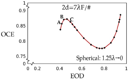
Figure 3.
OCE vs. EOD for a lens with the spherical aberration (ρ4-term) for a detector pixel size of 2d = 7λF/#. The amount of spherical aberration decreases from the middle-left region with the value of a40 = 1.25λ along the curve to the upper right corner with a40 = 0.
General features of the OCE vs. EOD curve in Figure 3 for large pixel 2d = 7λF/# are quite similar to those for the small pixel in Figure 1. The OCE values increase for very small values of the EOD and for large values of the EOD with the increasing amount of aberration. A peak and a valley arise between these two regions, like the shape in Figure 1. The amount of spherical aberration decreases from the lower left corner with the value of a40 = 1.25λ along the curve to the upper right corner with a40 = 0.
In the absence of aberration, the maximum energy on the detector enclosed by the square pixel is 0.95. When the amount of spherical aberration increases from 0 to a40 = 1.25λ, the EOD decreases from about 0.95 to 0.4 when using a pixel size of 2d = 7λF/#. When there is no aberration, the OCE achieves the value of 0.89. The OCE first rapidly decreases with increasing amount of aberration, achieving the valley bottom of the OCE = 0.78 at the EOD = 0.80. The OCE then, with a slope of about (minus) 45 degrees, approaches and forms a rounded peak, nearly equal to the case of no aberration around the aberration value of a40 = 1λ. When the aberration further increases, about an average value is achieved for the OCE, equal to 0.84 for the EOD of 0.4. Here we note that the OCE is proportional to the EOD in about one half of the EOD interval and inversely proportional in the other half. They are not correlated.
Next, we endeavor to explain the first one-third of the curve for the small EOD values, featuring a narrow, sharp OCE peak. The prf-s corresponding to the three points around the local peak (Points A, B, and C) are plotted in Figure 4. Point response functions prf-s for Points A, B, and C have a similar profile across the pixel surface. For these points, the EOD increases from 0.42 through 0.47 to 0.50. The prf(0) and prf(0.5) for Point A are 0.421 and 0.25, resulting in their difference of 0.17. The prf(0) and prf(0.5) for Point B are 0.47 and 0.31, resulting in their difference of 0.16. Even so, Point A has a lower EOD value than Point B. This leads to a relative higher variation of the EOD across the pixel surface and therefore a lower OCE value for Point A.
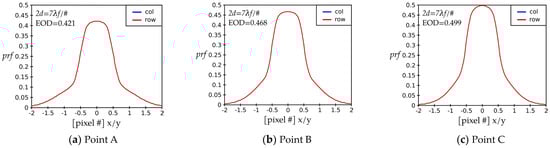
Figure 4.
The instrument point response function prf corresponding to selected points in Figure 3 as a function of two orthogonal directions, x and y, or rows and columns, for the case of spherical aberration. We model a case where the detector pixel size equals 7λF/#. With an increase in the aberration, the energy spreads out. The energy on detector EOD for the same pixel size decreases with increasing amount of aberration. The figures are arranged in order of increasing energy on the detector, which corresponds to a decreasing amount of aberration. Due to the symmetry of the problem, the red line overlaps over the blue line.
The prf-curve corresponding to Point C has the highest EOD value (that is, prf(0)), and a more narrowly formed cone at the center than the other two. Additionally, it also features a relatively larger difference in the prf-values between the center and edge of the detector pixel than that of Point B. The edge value is 0.32, and the center value is 0.5, resulting in the difference from the center to the edge of 0.18. Thus, Point C presents a larger variation in the prf-values across the pixel surface. Therefore, Point C ends up having a somewhat lower OCE value than Point B.
In the presence of 3rd order spherical aberration in an otherwise ideal lens-optical detector combination, the EOD decreases in the presence of aberration because the energy in the central spot is being pushed out to the outer rings. The amount of energy that is incident on a given pixel and the average prf across the detector determine the relationship between EOD and OCE. For a different size pixel, with its value somewhere between 2d = 3λF/# and 2d = 7λF/#, the initial points and the end points would be lying between the corresponding points on Figure 1 and Figure 3. The OCE-vs-EOD curve would exhibit a shape similar to the two limiting cases presented here and lying in-between them.
4. Coma-y: a31 ρ3sinθ
4.1. Coma-y for Small Pixel Size, 2d = 3λF/#
We present the OCE vs. the EOD graph for the case of coma aberration for small pixel size 2d = 3λF/# in Figure 5. In the absence of aberration, the maximum energy on the detector enclosed by the square pixel is 0.88. When the amount of coma aberration increases from a31 = 0 to a31 = 1.25λ, the EOD decreases from about 0.88 to 0.25 when using a pixel size of 2d = 3λF/#. Except for the outer regions of the interval under study, the increase in the amount of aberration appears to affect the EOD moderately.
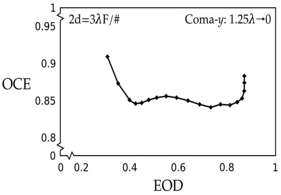
Figure 5.
OCE vs. EOD for a lens with the coma aberration (a31 = ρ3sinθ) for a detector pixel size of 2d = 3λF/#. The amount of coma aberration decreases from the upper left corner with the value of a31 = 1.25λ along the curve to the right middle area with a31 = 0.
When there is no aberration, the OCE achieves the value of 0.88. At first the OCE sharply, nearly vertically, decreases with increasing amount of aberration; then, it rolls off to an approximately constant value, at about OCT = 0.85. It features two small valleys of OCT = 0.84, at EOD = 0.74 and 0.41. The OCE starts to increase again with increasing aberration at about a31 = 1λ. When the aberration further increases to a31 = 1.25λ, the OCE increases, achieving a value of 0.91 for an EOD of 0.25.
Here we note that the OCE is roughly independent of the EOD for the middle half of the EOD interval. During the first quarter of the interval, it is inversely proportional. It is proportional in the last quarter. We can also say that the OCE and the EOD are independent of each other in the case of the coma aberration. We may simply observe that coma affects differently the EOD and the OCE. We may simply observe that the OCE and the EOD are not correlated under the effects of coma for small pixel size in the study.
4.2. Coma-y with Large Pixel Value, 2d = 7λF/#
We present the OCE vs. the EOD graph for the case of coma aberration for large pixel size 2d = 7λF/# in Figure 6. In the absence of aberration, the maximum energy on the detector enclosed by the square pixel is 0.95. When the amount of coma aberration increases from a31 = 0 to a31 = 1.25λ, the EOD decreases from about 0.96 to 0.6 when using a pixel size of 2d = 7λF/#, while the OCE decreases from 0.95 to 0.83.
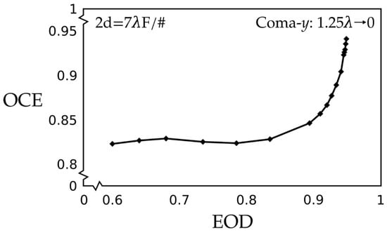
Figure 6.
OCE vs. EOD graph for a lens with the coma aberration (a31 ρ3sinθ) for a detector pixel size of 2d = 7λF/#. The amount of coma aberration decreases from the lower left corner with the value of a31 = 1.25λ along the curve to the upper right corner with a31 = 0.
In absence of aberration, the OCE achieves the value of 0.95. From there, it first rapidly decreases with increasing amount of aberration, arriving to its elbow at the EOD = 0.88. The OCE then remains approximately constant with increasing aberration, achieving a small hump for the aberration value of a31 = 1λ for the EOD of 0.68. When the aberration further increases, the OCE decreases to 0.825 for the EOD value of 0.6.
Here we note that the OCE is roughly independent of the EOD for more than one half of the EOD interval. During about the last third of the interval, the OCE is proportional to the EOD. We may simply conclude that for large amounts of coma aberration, the OCE and the EOD are independent of each other. For small amounts of the coma aberration, the OCE is proportional to the EOD.
5. Astigmatism: a22 ρ2cos2θ
5.1. Astigmatism a22 ρ2cos2θ for Small Pixel Size, 2d = 3λF/#
We present the OCE vs. the EOD graph for the case of astigmatism aberration for small pixel size 2d = 3λF/# in Figure 7.
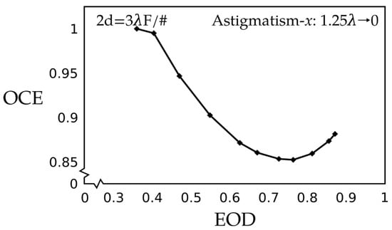
Figure 7.
OCE vs. EOD graph for a lens with the astigmatism aberration (a22 ρ2cos2θ) for a detector pixel size of 2d = 3λF/#. The first zero of the Bessel function is located at 1.22 λF/#. In the absence of aberration, the pixel encloses somewhat more than the Airy disc diameter. The amount of astigmatism aberration decreases from the upper left corner with the value of a22 = 1.25 λ along the curve to the right middle area with a22 = 0.
In the absence of aberration, the maximum energy on the detector enclosed by the square pixel is 0.88. When the amount of astigmatism aberration increases from a22 = 0 to a22 = 1.25 λ, the EOD decreases from about 0.88 to 0.35 when using a pixel size of 2d = 3λF/#. When there is no aberration, the OCE achieves the value of 0.88. For an initial short interval, the OCE first smoothly decreases with increasing amount of astigmatism aberration, achieving the minimum value of 0.85 for the EOD = 0.74; afterwards, it climbs with about a 45-degree slope to its rounded peak at practically 1, while the EOD is only 0.35 for the aberration value a22 = 1.25λ.
For about the first two-thirds of the EOD interval, the OCE is inversely proportional to the EOD. During the last third, the OCE is proportional to the EOD. We note that the general curve has the same shape as the central part of the corresponding spherical aberration curve. We may simply observe that the OCE and the EOD are not correlated for small pixel sizes.
5.2. Astigmatism a22 ρ2cos2θ for Large Pixel Value, 2d = 7λF/#
We present the OCE vs. the EOD graph for the case of astigmatism aberration for large pixel size 2d = 7λF/# in Figure 8.
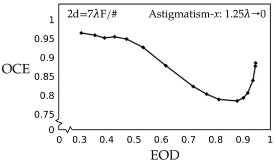
Figure 8.
OCE vs. EOD graph for a lens with the astigmatism aberration (a22 ρ2cos2θ) for a detector pixel size of 2d =7λF/#. The first zero of the Bessel function is located at 1.22 λF/#. In the absence of aberration, the pixel encloses 2.87 Airy discs (nearly 3). The amount of astigmatism aberration decreases from the upper left corner with the value of a22 = 1.25λ along the curve to the right middle area with a22 = 0.
In the absence of aberration, the maximum energy on the detector enclosed by the square pixel is 0.95. When the amount of astigmatism aberration increases from a22 = 0 to a22 = 1.25λ, the EOD decreases from about 0.95 to 0.35 when using a pixel size of 2d = 7λF/#. When there is no aberration, the OCE achieves the value of 0.88. For an initial short interval, the OCE first smoothly decreases with increasing amount of astigmatism aberration, achieving the minimum value of OCE = 0.78 at the EOD = 0.86; afterwards, it climbs with about a 45-degree slope to its elongated rounded peak for the OCE = 0.97 at the EOD = 0.3, for the aberration value a22 = 1.25λ.
For about the fourth or fifth EOD interval, the OCE is inversely proportional to the EOD. During the last fifth, the OCE is proportional to the EOD. We note that the general curve has a distorted shape of the central part of the corresponding spherical aberration curve. We may observe that the OCE and the EOD are not correlated for large pixels.
6. Defocus/Power: a20 ρ2
6.1. Defocus/Power a20 ρ2 for Small Pixel 2a = 3λF/#
We present the OCE vs. the EOD graph for the case of defocus aberration for small pixel size 3λF/# in Figure 9. In the absence of defocus aberration, the maximum energy on the detector enclosed by the square pixel is 0.88. When the amount of defocus aberration increases from a20 = 0 to a20 = 1.25λ, the EOD decreases from about 0.88 to 0.31 when using a pixel size of 2d = 3λF/#. When there is no aberration, the OCE achieves the value of 0.88. The OCE first smoothly decreases with increasing amount of aberration, achieving a minimum of 0.82 for the EOD of 0.62. From there, the curve looks like a quadratic function tilted to the side.
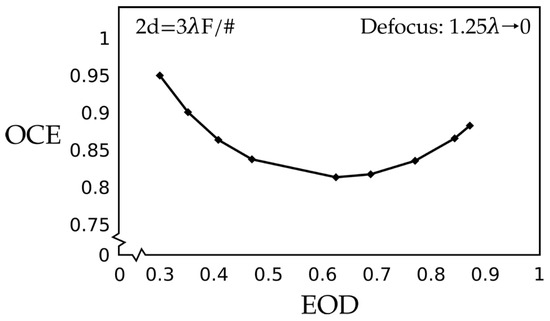
Figure 9.
OCE vs. EOD graph for a lens with the defocus aberration (a20 ρ2) for a detector pixel size of 2d = 3λF/#. The amount of defocus aberration decreases from the upper left corner with the value of a20 = 1.25 λ along the curve to the right middle region with a20 = 0.
When the aberration further increases, the highest value is achieved for the OCE of 0.95 at the EOD of 0.31. Here we note that for defocus aberration, the OCE is proportional to the EOD for half of the EOD interval and inversely proportional to the other half. We may simply observe that they are not correlated.
6.2. Defocus/Power with Large Pixel Value, 2d = 7λF/#
We present the OCE vs. the EOD graph for the case of defocus aberration for large pixel size 2d = 7λF/# in Figure 10.
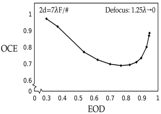
Figure 10.
OCE vs. EOD graph for a lens with the defocus aberration (a20) for a detector pixel size of 7λF/#. The amount of defocus aberration decreases along the curve from the upper left corner through the minimum and then to the upper right corner with a20 = 0.
In the absence of defocus aberration, the maximum energy on the detector enclosed by the square pixel is 0.95. When the amount of defocus aberration increases from a20 = 0 to a20 = 1.25λ, the EOD decreases from about 0.95 to 0.3 when using a pixel size of 2d = 7λF/#. In the absence of aberration, the OCE achieves the value of 0.89. It first rapidly decreases with increasing amount of aberration, achieving a minimum of 0.68 at the EOD of 0.77. From there, the curve looks like a quadratic function with unequal sides. The OCE graph vs. EOD graph increases with about a 45-degree inclination angle with increasing aberration. When the aberration further increases, the highest value is achieved for the OCE, equal to 0.98 for the EOD of 0.31.
Here we note that for the defocus aberration, the OCE is proportional to the EOD for a quarter of the EOD interval. It is inversely proportional for about three-quarters of the EOD interval. We may simply observe that the OCE and the EOD are not correlated for the defocus in the case of the large pixel.
7. Discussion
7.1. Spherical Aberration
We present the OCE vs. the EOD graph for the case of spherical aberration for two pixel sizes 2d = 3λF/# and 2d = 7λF/# in Figure 11. The first point on the left of each graph corresponds to the amount of spherical aberration, a40 = 1.25λ, while the last point on the right of the graph corresponds to the case of no aberration, a40 = 0.
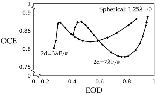
Figure 11.
OCE vs. EOD graph for the case of spherical aberration for two pixel sizes 2d = 3λF/# and 2d = 7λF/#. The first point on the left of each graph corresponds to the amount of spherical aberration, a40 = 1.25 λ, while the last point on the right of each graph corresponds to the case of no aberration, a40 = 0.
The most interesting aspect in comparison of these two graphs is that they are quite similar in general shape. The graph for the small pixel appears to be compressed along the OCE axis and displaced toward smaller values along the EOD axis. They both feature peaks, corresponding to the absence of aberration that has nearly the same value, OCE = 0.87. The peak is displaced for the smaller pixel by about DEOD = 0.12. Both graphs also include valleys, displaced by DEOD = 0.2 and DOCE = 0.12. The minimum for the larger pixel is deeper and displaced to larger EOD values.
In the absence of aberration, the maximum energy on the detector enclosed by the square pixel is 0.88 for a small pixel size of 2d = 3λF/#. The maximum energy on the detector for the larger pixel size of 2d = 7λF/# increases to 0.95. This increment of 0.07 is reasonable because a larger pixel encloses more energy for an aligned system. In the absence of aberration, the pixel size has minimal effects on possible displacement of the optical axis on the collected energy or other environmental effects. From the local maximum characterized by no aberration, graphs then decrease to a valley, with the graph for the large pixel size having a slope larger than 45 degrees and that for the smaller pixel having a smaller slope.
When the amount of spherical aberration increases from a40 = 0 to a40 = 1.25λ, the EOD decreases to 0.25 for a pixel size of 2d = 3λF/#. At the same time, the EOD increases to 0.4 for pixel size 2d = 7λF/#. This increase of 0.15 for the larger pixel in the enclosed energy is also reasonable because a large amount if spherical aberration spreads the energy to a larger spot. A small pixel intercepts a smaller fraction of energy of a large spot than a large pixel; therefore, the small pixel is impacted by aberration more than the large one. The increase in the EOD for the large pixel is twice the increase for the small pixel. Because the displacement of the optical axis still allows a large amount of energy to be intercepted.
7.2. Coma-y
We present the curve of the OCE vs. the EOD graph for the case of coma-y aberration for two pixel sizes (2d = 3λF/# and 2d = 7λF/#) in Figure 12. The first point on the left of each graph corresponds to the amount of coma, a31 = 1.25 λ, while the last point on the right of the graph corresponds to the case of no aberration, a31 = 0.
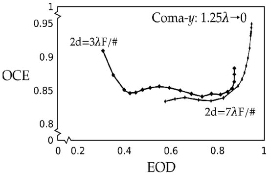
Figure 12.
OCE vs. EOD graph for the case of coma-y aberration for two pixel sizes 2d = 3λF/# and 2d = 7λF/#. The first point on the left of each graph corresponds to the amount of coma aberration, a31 = 1.25λ, while the last point on the graph corresponds to the case of no aberration, a31 = 0. For a large portion of the aberration under study, from about a31 = 0.25λ to roughly a31 = 1.25λ, the OCE seems to be independent of the amount of aberration.
In the absence of aberration, the EOD enclosed by the square pixel is 0.88, for the small pixel size 2d = 3λF/#. In the absence of aberration, the maximum energy on the detector enclosed by the square pixel is 0.95 for the case of the large pixel size, 2d = 7λF/#. This is a small shift of 0.07. When the amount of coma aberration increases to a31 = 1.25λ, the EOD decreases from to 0.25 in the case of a small pixel size 2d = 3λF/#. When the amount of coma aberration increases from a31 = 0 to a31 = 1.25λ, the EOD decreases to 0.6 when using a pixel size of 2d = 7λF/#. When there is no aberration, the OCE achieves the value of 0.98 for the small pixel size 2d = 3λF/#. When there is no aberration, the OCE achieves a value of 0.95 in the case of the large pixel size 2d = 7λF/#.
For the small pixel size 2d = 3λF, the OCE initially sharply vertically decreases with increasing amounts of aberration, taking a sharp turn for the EOD value of 0.84. The OCE then rolls off to an approximately constant value, at about 0.85, with two small valleys of 0.84 at 0.77 and 0.41. F for the case of the large pixel size 2d = 7λF/#, the OCT initially nearly vertically rapidly decreases with increasing amount of aberration, taking a sharp turn at the EOD value of 0.84. The OCE then remains approximately constant, achieving a small hump for aberration value a31 = 1λ for the EOD of 0.68.
The OCE starts to increase again at the aberration of a31 = 1λ. When the aberration further increases, the OCE increases, achieving a value of 0.91 for an EOD of 0.25 for the small pixel size 2d = 3λF/#. When the aberration further increases, the OCE decreases to 0.825 for the EOD value of 0.60, for the case of the large pixel size 2d = 7λF/#.
For a large portion of the aberration under study, from about a31 = 0.25λ to roughly a31 = 1.25λ, the OCE seems to be independent of the amount of aberration. The EOD for the aberration a31 = 1.25λ nearly doubles from small (EOD = 0.32) to the large pixel (EOD = 0.60). This means that the coma is very sensitive to the pixel size for large aberrations. For a small amount of aberration, the EOD has low sensitivity on the coma aberration, while the OCE changes rapidly with the aberration.
7.3. Astigmatism
We present the curve of the OCE vs. the EOD graph for the case of astigmatism aberration for two pixel sizes 2d = 3λF/# and 2d = 7λF/# in Figure 13. The first point on the left on each graph corresponds to the amount of astigmatism aberration a22 = 1.25λ, while the last point on the right side of the graph corresponds to the case of no aberration.
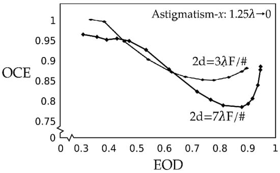
Figure 13.
OCE vs. EOD graph in the case of astigmatism aberration for two pixel sizes, 2d = 3λF/# and 2d = 7λF/#. The first point on the left of each graph corresponds to the amount of astigmatism aberration, a22 = 1.25λ, while the last point on the right of the graph corresponds to the case of no aberration, a22 = 0.
In the absence of aberration, the maximum energy on the detector enclosed by the square pixel is 0.88 for the small pixel size 2d = 3λF/#. In the absence of aberration, the maximum EOD enclosed by the square pixel is 0.89, for the case of the large pixel size 2d = 7λF/#. When the amount of astigmatism aberration increases from 0 to 1.25 λ, the EOD decreases from about 0.88 to 0.35 when using a pixel size of 2d = 3λF/#.
In the absence of aberration, the OCE achieves the value of 0.89 at the EOD of 0.88 for the small pixel size 2d = 3λF/#. When there is no aberration, the OCE achieves the value of 0.89 for the large pixel size 2d = 7λF/#. For the small pixel size 2d = 3λF/#, the OCE first slowly and smoothly decreases with increasing amount of aberration, achieving the minimum value of 0.85 at about 0.74. The OCE first rapidly decreases with increasing amount of aberration, achieving the minimum at 0.78 at EOD of 0.84, for the case of the large pixel size 2d = 7λF/#.
After the valley, the OCEs climb with an about 45-degree slope to rounded peaks at different heights. Practically 1 is achieved for the case of the small pixel size 2d = 3λF/#, at the EOD of only 0.35 for the aberration value 1.25 λ. In the case of the large pixel size 2d = 7λF/#, the slope is somewhat higher, but the curve rounds off sooner to a nearly horizontal extended hump around 1λ. When the aberration further increases, the OCE slowly increases to a value of 0.96 for the EOD of 0.31, for the case of the large pixel size 2d = 7λF/#.
The shapes of two astigmatism curves for the small and large pixel are, in general, quite similar. For the small amount of aberration, the OCE decreases together with the EOD, but more quickly for the large pixel than for the small one. Both curves attain a minimum, but the one for the larger pixel is achieved for a longer EOD value and it is deeper than for the small pixel. With an increasing amount of aberration, the OCE increases with the decreasing EOD. The interval of the EOD is about the same for both pixel sizes, except that graph is displaced by 0.03 to the longer EOD values for the larger pixel.
7.4. Defocus/Power
We present the OCE vs. EOD graph for the case of defocus aberration for two pixel sizes 2d = 3λF/# and 2d = 7λF/# in Figure 14. The first point on the left of each graph corresponds to the amount of defocus aberration a20 = 1.25λ, while the last point on the right of the graph corresponds to the case of no aberration.
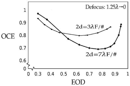
Figure 14.
OCE vs. EOD graph for the case of defocus aberration for two pixel sizes 2d = 3λF/# and 2d = 7λF/#. The first point on the left of each graph corresponds to the amount of defocus aberration, a20 = 1.25 λ, while the last point on the graph corresponds to the case of no aberration, a20 = 0.
In the absence of aberration, the maximum EOD enclosed by the square pixel is 0.88 for the small pixel size 2d = 3λF/#. In the absence of aberration, the maximum energy on the detector enclosed by the square pixel is 0.89; for the case of the large pixel size, 2d = 7λF/#. When the amount of defocus aberration increases to a20 = 1.25 λ, the EOD decreases to 0.31, when using a pixel size of 2d = 3λF/#. When the amount of defocus aberration increases from 0 to 1.25λ, the EOD decreases to 0.31, when using a pixel size of 2d = 7λF/#. The pixel size has no effect on the EOD for the large amount of defocus aberration.
When there is no aberration, the OCE achieves the value of 0.88 for the EOD value of 0.84 for the small pixel size 2d = 3λF/#. When there is no aberration, the OCE achieves the value of 0.89 for the EOD values of 0.95, for the case of the large pixel size 2d = 7λF/#.
The OCE first smoothly decreases with increasing amount of aberration, achieving a minimum at 0.82 for EOD of 0.62 for the small pixel size 2d = 3λF/#. The OCE rapidly decreases with increasing amount of aberration, achieving a minimum at 0.68 for the EOD of 0.77 in the case of the large pixel size 2d = 7λF/#.
From the minimum, the curve for the OCE looks like a quadratic function with unequal sides. When the aberration further increases, the highest value is achieved for the OCE, equal to 0.95 at the EOD of 0.31, for the small pixel size 2d = 3λF/#. From the minimum, the OCE curve increases with the increasing aberration. The highest OCE value achieved is equal to 0.99 for the EOD of 0.31, for the case of the large pixel size 2d = 7λF/#.
The shapes of two defocus curves for the small and large pixel are in general quite similar. For a small amount of aberration, the OCE decreases together with the EOD, but more quickly for the large pixel than for the small one. Both curves attain a minimum, but the one for the larger pixel is achieved for a longer EOD value, and it is deeper than for the small pixel. With the increasing amount of aberration, the OCE increases with the decreasing EOD. The OCE for the large pixel starts to climb up slowly to the highest possible value of 1, but it cuts off at 0.99 for the OCE final value. For the smaller pixel, the curve is still increasing sharply at the maximum aberration, achieving OCE = 0.94, while it slowly approaches to this value. The interval of the EOD is about the same for both pixel sizes, except that graph is displaced by 0.03 to the longer EOD values for the larger pixel.
8. Summary and Conclusions
In the cases of the individual aberration that we evaluated, we note that the effect of aberration is less pronounced on the OCE than on the EOD. Most importantly, the conventional wisdom would expect that the OCE increases with the EOD linearly regardless of the pixel size and the type of aberrations. In this work, we demonstrate for all aberrations that the OCE increases with the EOD for small amounts of aberration, except for the smaller pixel size in astigmatism, in which the asymmetrical nature of psf cannot be collected completely. However, as the amount of aberration reaches a certain point (as the EOD keeps getting smaller), the trend reverses and the OCE starts to increase. Furthermore, when the pixel is sufficiently large to include enough energy, this correlation is even more pronounced.
With respect to the pixel size, the most interesting aspect of the comparison of the OCE vs. the EOD graphs for two pixels under study is that they are quite similar; however, they appear to be compressed and slightly displaced along the EOD-axis.
The EOD is more sensitive to the amount of aberration than the OCE. The aberrations and their amount affect the EOD differently for both pixel sizes studied here. For smaller pixels, the aberration amount ranging from 0 to 1.25λ subtends quite a large interval on the EOD axis, from 0.25 to 0.95, while the OCE domain varies from 0.80 to 1. The width of the EOD interval is approximately the same for all aberrations studied here. The same amount of aberration, that is, aii = 1.25λ, decreases the EOD for the spherical to 0.24, the coma to 0.29, the defocus to 0.30, and the astigmatism to 0.34. Therefore, if the EOD is to be maximized while allowing some aberration, the astigmatism is the aberration to permit when imaging with a smaller pixel.
For the larger pixel, the aberrations cover quite a large interval on the EOD axis, while the OCE varies from 0.68 to 0.95. The width of the EOD interval is significantly different for all aberrations studied here. The same amount of aberration, that is, aii = 1.25λ, decreases the EOD for the defocus and the astigmatism to 0.31, for the spherical to 0.40, and the coma to 0.60. Therefore, if the EOD is to be maximized while allowing some aberration, the coma is the aberration to permit when imaging with the large pixel.
Based on these studies, we consider that the energy enclosed within the square pixel, the EOD, remains an interesting parameter but not necessarily the most informative one as an aid in design specifications. However, due to the high probability that the pixel center and the axis of the optical system are misaligned—for all pixels in the focal plane array—the energy that spills on the neighboring pixel is usually not lost to the signal. It is added to its nearest neighbors, where it most likely still contributes to the signal. This is particularly relevant for those cases where the small pixel intercepts small amounts of energy due to a large amount of aberration producing a large signal spread.
As a design guideline, then, we see that a small pixel 2d = 3λF/# results in a high OCE even for a large amount of aberration for all aberrations studied. For zero and very small amounts of aberration, the large pixel 2d = 7λF/# in general achieves a better OCE than the small pixel. In the intermediate aberration region, there does not appear to be much difference in the OCE for the two pixels studied here, except in the case of the spherical aberration, where a small pixel is preferable for most of the aberration interval.
In conclusion, for pixels larger than 2d = 3λF/#, a small pixel will feature better performance when expecting jitter, misalignment, and other environmental and unpredictable external conditions for all but minimal aberration. When counting on the perfect aberration-free design, the choice of lager pixel is expected to have better energy collection properties, but such design will be plagued by the deterioration of another figure-of-merit, the image resolution.
In the future, we intend to extend this study to a mixture of aberrations to mimic a realistic optical system as close as possible. In a follow-up publication, we will address a mixture of aberrations on the performance of an instrument in an environment subjected to jitter and misalignments. With that, the same amounts of aberrations will be applied to both refractive and reflective optical systems so that we can explore and have better insight over the OCE vs. EOD relationships. We also plan to apply this theory to other remote sensing instruments.
Author Contributions
All authors contributed equally to this MS. Conceptualization, Y.W. and R.M.; Investigation, Y.W.; Methodology, M.S.; Visualization, M.S.; Writing—original draft, M.S. and Y.W.; Writing—review and editing, M.S.; Writing—final, M.S. All authors have read and agreed to the published version of the manuscript.
Funding
This research received no external funding.
Institutional Review Board Statement
The study did not require ethical approval or institutional review.
Informed Consent Statement
The study did not require informed consent.
Data Availability Statement
The data presented in this study are included in this study.
Acknowledgments
MS thanks RMA and BBM for helpful discussions.
Conflicts of Interest
The authors declare no conflicts of interest.
References
- Strojnik, M.; Bravo-Medina, B.; Martin, R.; Wang, Y. Ensquared energy and optical centroid efficiency in optical sensors: Part 1, Theory. Photonics 2023, 10, 254. [Google Scholar] [CrossRef]
- Muñoz, J.; Strojnik, M.; Paez, G. Phase recovery from a single undersampled interferogram. Appl. Opt. 2003, 42, 6846–6855. [Google Scholar] [CrossRef] [PubMed]
- Brady, D.J.; Gehm, M.E.; Stack, R.A.; Marks, D.L.; Kittle, D.S.; Golish, D.R.; Vera, E.M.; Feller, S.D. Multiscale gigapixel photography. Nature 2012, 486, 386–389. [Google Scholar] [CrossRef] [PubMed]
- Sroubek, F.; Kamenicky, J.; Lu, Y.M. Decomposition of Space-Variant Blur in Image Deconvolution. IEEE Signal Process. Lett. 2016, 23, 346–350. [Google Scholar] [CrossRef]
- Catrysse, P.B.; Wandell, A.B. Optical efficiency of image sensor pixels. J. Opt. Soc. Am. A 2002, 19, 1610–1620. [Google Scholar] [CrossRef] [PubMed]
- Li, X.; Suo, J.; Zhang, W.; Yuan, X.; Dai, Q. Universal and flexible optical aberration correction using deep-prior based deconvolution. In Proceedings of the 2021 IEEE/CVF International Conference on Computer Vision (ICCV), Montreal, BC, Canada, 11–17 October 2021; pp. 2593–2601. [Google Scholar]
- Kerepecký, T.; Šroubek, F. D3Net: Joint demosaicking, deblurring, and deringing. In Proceedings of the 2020 25th International Conference on Pattern Recognition (ICPR), Milan, Italy, 10–15 January 2021; pp. 1–8. [Google Scholar]
- Welford, W.T. Aberrations of the Symmetrical Optical System; Academic Press: London, UK, 1974; p. 120. [Google Scholar]
- Born, M.; Wolf, E. Principles of Optics, 7th ed.; Cambridge University Press: Cambridge, UK, 1999. [Google Scholar]
- Mahajan, V. Aberration Theory Made Simple; SPIE: Bellingham, WA, USA, 1991; Volume TT6, p. 11. [Google Scholar]
- Smith, W. Modern Optical Engineering, 4th ed.; McGraw Hill: New York, NY, USA, 2008; p. 311. [Google Scholar]
Disclaimer/Publisher’s Note: The statements, opinions and data contained in all publications are solely those of the individual author(s) and contributor(s) and not of MDPI and/or the editor(s). MDPI and/or the editor(s) disclaim responsibility for any injury to people or property resulting from any ideas, methods, instructions or products referred to in the content. |
© 2024 by the authors. Licensee MDPI, Basel, Switzerland. This article is an open access article distributed under the terms and conditions of the Creative Commons Attribution (CC BY) license (https://creativecommons.org/licenses/by/4.0/).