Abstract
Coaxial bioreactors are known for effectively dispersing gas inside non-Newtonian fluids. However, due to their design complexity, many aspects of their design and function, including the relationship between hydrodynamics and bioreactor efficiency, remain unexplored. Nowadays, various numerical models, such as computational fluid dynamics (CFD) and artificial intelligence models, provide exceptional opportunities to investigate the performance of coaxial bioreactors. For the first time, this study applied various machine learning models, both classifiers and regressors, to predict the torque generated by a coaxial bioreactor. In this regard, 500 CFD simulations at different aeration rates, central impeller speeds, anchor impeller speeds, and rotating modes were conducted. The results obtained from the CFD simulations were used to train and test the machine learning models. Careful feature scaling and k-fold cross-validation were performed to enhance all models’ performance and prevent overfitting. A key finding of the study was the importance of selecting the right features for the model. It turns out that just by knowing the speed of the central impeller and the torque generated by the coaxial bioreactor, the rotating mode can be labelled with perfect accuracy using k-nearest neighbors (kNN) or support vector machine models. Moreover, regression models, including multi-layer perceptron, kNN, and random forest, were examined to predict the torque of the coaxial impellers. The results showed that the random forest model outperformed all other models. Finally, the feature importance analysis indicated that the rotating mode was the most significant parameter in determining the torque value.
1. Introduction
Mechnical agitators equipped to bioreactors are mainly used to enhance mass and heat transfer within the bioreactor. These systems are crucial in sectors ranging from pharmaceutical production to wastewater treatment. The effectiveness of these bioreactors is greatly influenced by their power consumption, particularly in terms of mixing intensity and homogeneity. Efficient power consumption is key to achieving optimal performance in agitated bioreactors [1].
The power drawn value is the required energy at a specific time to create fluid bulk motion [2]. Under ungassed conditions, stirrer speed, impeller shape and size, the geometry of the tank, and fluid properties can affect the power requirement. However, the ungassed power drawn shows a strong dependency on the impeller diameter and stirrer speed. Under turbulent flow regime, the ungassed power drawn is dependent on the fluid density and is independent of the fluid viscosity. Typically, the required power decreases with gas dispersion. This can be attributed to a reduction in the fluid mixture density in the presence of the gas bubble [3]. However, the main reason for the reduction in power drawn upon aeration is the formation of gas-filled cavities in the impeller region, which reduces the stirrer rotation drag, and as a result, the transmitted power from the impeller to the fluid decreases [4]. Radial-flow impellers, such as Rushton impellers, exhibit a higher amount of power reduction upon aeration, and the power consumption of the Rushton impeller reduces by about 50% under aeration [5].
For thedown-pumping axial-flow impellers, the power reduction due to aeration is small at low gas flow rates because, under this condition, the flow pattern is defined as an indirect loading flow regime. When the flow regime changes from an indirect to a direct loading regime at higher gas flow rates, the power drop due to aeration is substantial [6]. The power consumption of down-pumping axial-flow impellers is less than that of radial-flow impellers [5]. However, since they have a very unstable cavity structure, they encounter torque fluctuations [7,8]. In order to solve this problem, some researchers prefer using up-pumping impellers [9,10].
The effect of fluid rheology on power reduction is also significant. By increasing the fluid viscosity, the amount of power reduction increases. At the same aeration rate and impeller speed, the transmitted power to a non-Newtonian fluid is less than that of a Newtonian fluid [11,12]. In a non-Newtonian fluid, the viscosity changes with the shear rate. Hence, studying the power consumption in a non-Newtonian fluid is more complex than in a Newtonian fluid. Even with high turbulence mixing of the pseudoplastic fluids, the bulk fluids circulate slowly and consume less power than the fluid near the impeller region [13,14].
The coaxial bioreactor is a type of mixing system particularly designed for dispersing gas in non-Newtonian fluids [15,16]. These systems consist of two independent agitators. The one located at the center of the vessel is known as the central impeller, and the other is termed the close-clearance impeller [17]. The power consumption for the coaxial mixer in the counter-rotating mode is higher than that in the co-rotating mode [18].
Rahimzadeh et al. [17] conducted a comprehensive study on the power consumption of coaxial mixers. They showed a relationship between power reduction during aeration and the overall efficiency of mixing. In addition, they uncovered an intricate correlation between the rotating mode and the torque generated by the anchor impeller. Designing an accurate master power curve remains a significant challenge in this field, particularly for aerated coaxial mixers. In response to this challenge, Barros et al. [19] proposed new parameters for equivalent impeller diameter and rotational speed for a coaxial mixer containing yield-pseudoplastic fluids. They were able to accurately calculate the power number and Reynolds number of the system. Therefore, they successfully developed a master power curve. In another attempt, Sharifi et al. [20] successfully predicted the power curve for a coaxial mixer equipped with a dual central impeller and an anchor. Their research also demonstrated the influence of the central impeller type on power reduction during aeration.
Research on applying artificial intelligence to analyze mixing systems is still in its nascent stages, with only a handful of studies published to date [21]. Among these, the use of the random forest method has shown promising results. Kumar et al. [22] demonstrated the potential of this method in developing a predictive model for the segregation index in particulate mixing. Based on our comprehensive literature review, only two studies have been published on the application of neural networks in coaxial mixers [23,24]. Barros et al. [23] employed an artificial neural network (ANN) to predict the mass transfer coefficient in a coaxial bioreactor. They adopted two strategies: initially, they designed an ANN with two hidden layers, and subsequently, they implemented an ensemble neural network. Their findings indicated that the performance of the ensemble neural network was notably superior. In a more recent study, Yang et al. [24] utilized an artificial neural network to predict the optimal speed of the central impeller for achieving complete dispersion in a coaxial mixer containing a Newtonian fluid. Their model was structured with a single hidden layer comprising 11 neurons.
The use of artificial neural networks has also proven effective in predicting the master power curve. Bibeau et al. [25] implemented the cross-validation method within their ANN model to mitigate overfitting issues and to predict the power curve of a single-phase mixing tank. Additionally, artificial intelligence methods have been instrumental in enhancing the performance and efficiency of mixing systems. Research indicates that utilizing ANN models or evolutionary algorithms can address multi-objective optimization challenges. In fact, these methods are capable of determining the most efficient operating conditions, thereby optimizing performance while minimizing power consumption [26,27].
In many biochemical applications, determining the maximum allowable power consumption and impeller speed is crucial. To address this, our study introduces, for the first time, various machine learning methods developed to identify the optimal operating conditions and predict the torque generated by a coaxial bioreactor. In this study, the computational fluid dynamics method (CFD) was used to find the torque of a coaxial bioreactor. The system’s performance was evaluated under different conditions, including varying aeration rates, central and anchor impeller speeds, and rotational modes, in terms of power consumption. Moreover, the effectiveness of different machine learning methods in classifying the coaxial bioreactor into different rotating modes and predicting the torque generated by the mixing system was assessed.
2. Methods
2.1. Experiments
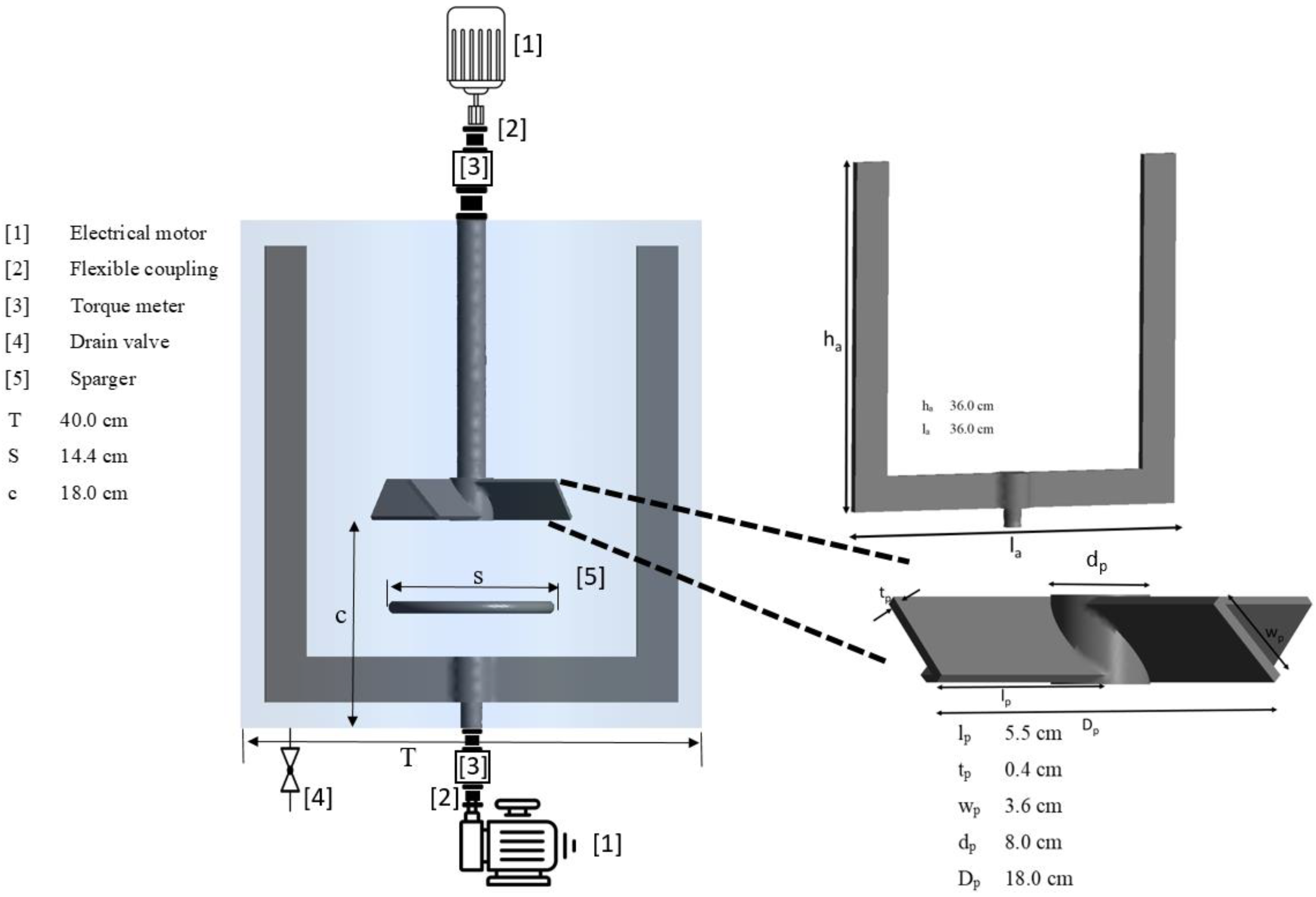
As per Figure 1, a mixing vessel was fabricated. The cylindrical vessel was filled with liquid to a height equivalent to the vesssel diameter. Therefore, the liquid volume was about 50.0 L. Two impellers were mounted on each shaft. As illustrated in Figure 1, the anchor impeller was fixed to the bottom shaft, and a pitched blade impeller in the upward-pumping direction was fixed to the top shaft as a central impeller. Each shaft was able to rotate independently in the same or opposite directions (co-rotating and counter-rotating modes). Air with a flow rate of 6 L/min was fed through the sparger. The procedure for power consumption calculation has been discussed in detail in our previous publications [17].
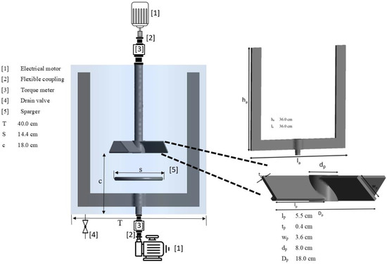
Figure 1.
Experimental setup.
A 0.5 wt% Carboxymethyl cellulose (CMC) solution was prepared, and its rheological properties were examined using the Bohlin C-VOR Rheometer 150 (Malvern Instruments, UK). The power-law non-Newtonian model was fitted to the data obtained from the rheometer at a temperature of . Hence, the consistency index (k) and power law index (n) were found to be 2.36 Pa sn and 0.65, respectively.
2.2. Computational Fluid Dynamics
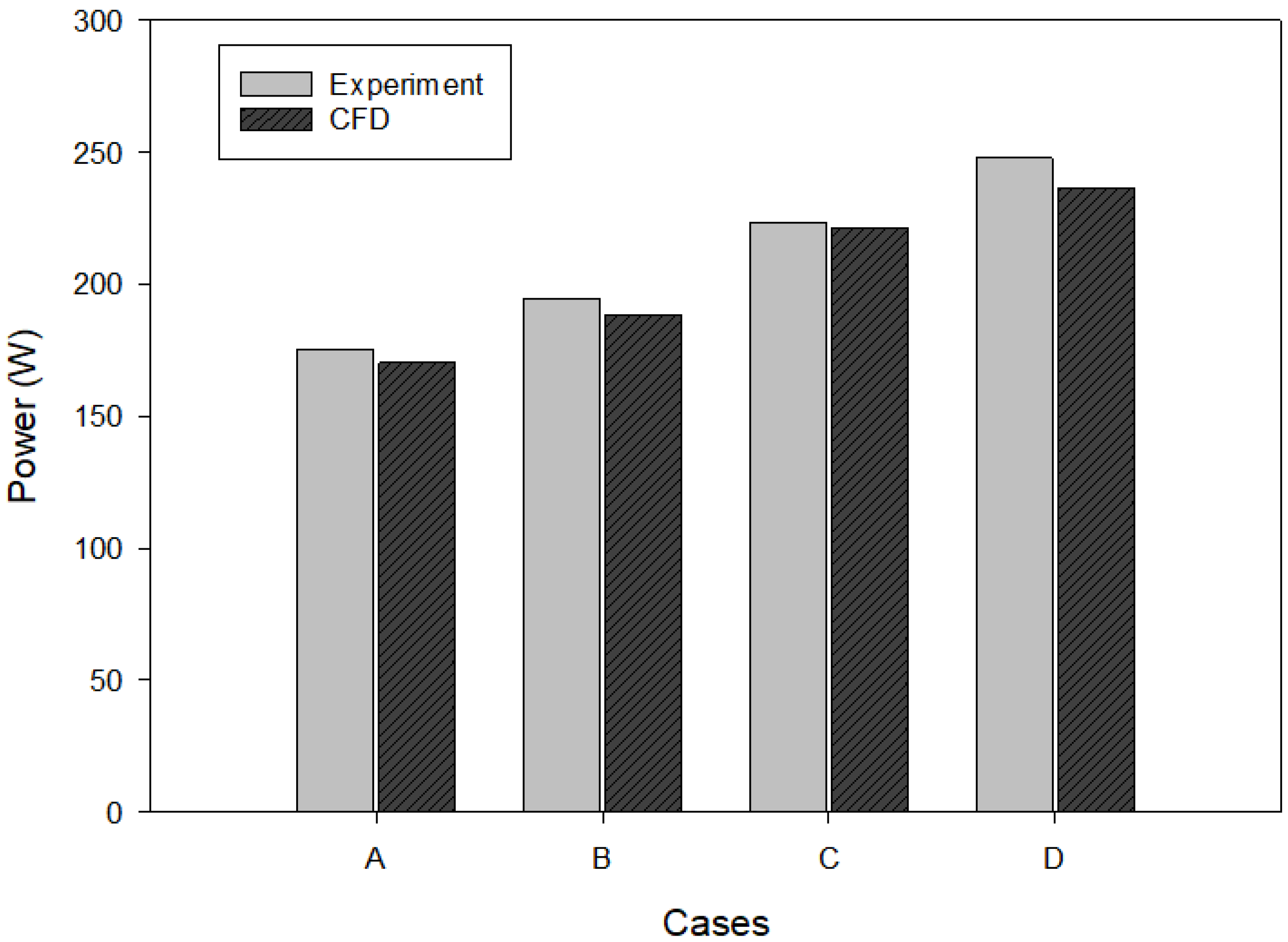
As previously discussed [17], we utilized ANSYS FLUENT 2022R2 software to develop a numerical model for examining the fluid dynamics within the aerated coaxial bioreactor. For a coaxial mixer with a volume of 50.0 L, the numerical model validation test based on the power consumption was carried out and presented in Figure 2. As shown in this figure, the numerical model was able to replicate the experimental data with satisfactory accuracy.
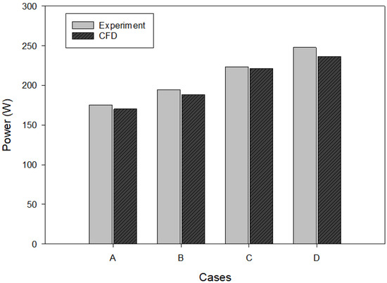
Figure 2.
Numerical model validation (Na = 10 rpm, Q = 0.8 L/min, 0.5 wt% CMC). Case A: Nc = 200 rpm, Case B: Nc = 240 rpm, Case C: Nc = 270 rpm, and Case D: Nc = 300 rpm.
In this research, we numerically developed a scaled-down model of a coaxial bioreactor by maintaining complete geometrical similarity and a scale factor of 0.5. As illustrated in Figure 2, the numerical model, sized at 50.0 L, was validated against experimental results. Consequently, the developed numerical model was size-independent and could be applied to a smaller scale. In fact, to minimize computation time, all CFD simulations were conducted using the small-scale coaxial mixer. A fluid volume of approximately 6.3 L was encapsulated within this small-scale bioreactor. A total of 500 CFD simulations were conducted under various operating conditions. All of the CFD simulations were performed on the Niagara supercomputer at the SciNet HPC Consortium. The operating conditions employed in this study are listed in Table 1.

Table 1.
The operating conditions used for the CFD simulations of a coaxial bioreactor with a volume of 6.3 L.
2.3. Machine Learning Model
All the data derived from the CFD simulations were utilized to train and test the machine learning models. As indicated by the data in Table 2, the features vary significantly in magnitude. Consequently, scaling the dataset was necessary. In this study, the MinMax normalization method was employed for dataset scaling [28]. Therefore, all features were scaled to fit within the range of zero to one, as follows:
Table 2.
Tuning of the k parameter in the kNN classifier across different cross-validation folds.
In this equation, and are the scaled and original data, respectively. Furthermore, the k-fold cross-validation method was employed to enhance the performance of the various machine learning algorithms and reduce the risk of overfitting problems.
To assess the performance of different machine learning models, various criteria were systematically investigated. Specifically, the mean square error (MSE) was employed to examine the accuracy of the proposed regression models:
In this equation, and are the actual and predictive responses, respectively.
Another parameter used to evaluate the performance of the regression model was R2 [29]:
In this equation, is the sum of the squared differences between the actual and predicted responses, and represents the total sum of squares variance in the actual and predicted responses. The value of the R2 score ranges between zero and one. However, a negative value for the predictive R2 is possible. This occurs when the variance in the test data exceeds that of the training data, indicating that the test data falls outside the training data’s range, and thus the model exhibits poor generalization [30].
For the evaluation of the classification models, the confusion matrix was calculated. This matrix encompassed four primary elements: true positive (TP), true negative (TN), false positive (FP), and false negative (FN). TP and TN represent cases where the model accurately predicted positive and negative classes, respectively. Conversely, FP and FN denote instances where the model erroneously predicted the classes. Based on the data obtained from the confusion matrix, the accuracy of each classification model was calculated [31]:
2.3.1. Classification Models
In this study, two supervised models were deployed to classify the coaxial mixer into two categories: co-rotating and counter-rotating modes. The k-nearest neighbors (kNN) model was employed as an instance-based method. This approach entails that the model’s predictions for the classes were based on instances from the training data. Consequently, for new instances, the model compared them with previously stored data [32].
In this study, the Euclidean distance metric was utilized to measure the distance between two data points in the k-nearest neighbors (kNN) algorithm. The classification of a test instance was determined based on the proximity of its nearest neighbors. For example, when the k value was set to 5, the algorithm identified the five nearest instances to the test data point within the feature space. Subsequently, the class of the test instance was predicted based on the majority class among these five neighbors. It is important to note that the selection of k was critically influential on the kNN model’s performance. A k value that was too small could have made the model susceptible to noise in the dataset, potentially leading to overfitting. On the contrary, a k value that was excessively large may have included points that were comparatively distant from the test instance, causing underfitting and poor generalization to new data points [33].
The support vector machine (SVM) model is a robust approach for binary classification tasks. In this research, the SVM model was employed to distinguish between the co-rotating and counter-rotating operational modes of the coaxial bioreactor. The SVM model is known for its capacity to identify the optimal linear hyperplane that maximizes the margin between two classes [34]. Therefore, the linear hyperplane serves as an efficient decision boundary for separating the co-rotating and counter-rotating modes. Mathematically, the decision boundary for an SVM with a linear kernel can be expressed as:
where is the weight vector and represents the feature vector.
Margins were determined based on the support vectors. Support vectors are the data points that are closest to the decision boundary, and are crucial for defining the hyperplane. One of the advantages of the SVM method is its reliance solely on these support vectors for model construction. Therefore, only these instances need to be remembered by the SVM model [34].
The distance between the margins, often referred to as the margin width, is given by the following equation [35]:
However, achieving this maximization is a sophisticated task. Thus, instead of Equation (3), the following equation can be minimized [35]:
where C represents the regularization. When C is set to zero, the model is referred to as having a hard margin. It means that no misclassification is tolerated. However, as C increases, the SVM becomes more tolerant of misclassifications (soft margin). To solve this optimization problem, the sequential minimal optimization (SMO) algorithm was frequently employed. SMO breaks the problem down into smaller sub-problems and makes the computation significantly efficient [36].
It is worth noting that most of the time, the relationship between classes is not linearly separable. To address this problem, the input data can be mapped to a higher-dimensional space where the classes are linearly separable. However, this transformation is computationally intensive. To overcome this problem, SVMs employ a powerful technique known as the kernel trick. For this purpose, there are many kernels available, such as polynomial, Gaussian, and sigmoid [37].
2.3.2. Regression Models
In this study, the torque produced by the coaxial mixer was predicted based on various operational parameters such as aeration rate, central impeller speed, anchor impeller speed, and rotating modes. By considering the rotating mode as a feature set, the complexity of the predictive modeling task increased significantly. To address this challenge, it was crucial to normalize all the input variables. In this study, various machine learning approaches were employed, including multi-layer perceptron (MLP), k-nearest neighbour (kNN), and random forest.
The MLP, also known as an artificial neural network (ANN), typically comprises multiple layers: an input layer, several hidden layers, and an output layer. Each layer consists of a number of neurons. In this study, a fully interconnected network was created. The input layer received all the feature variables, while the output layer was designed to predict the torque. In this model, each neuron computed a weighted sum of its inputs, added a bias, and then applied an activation function to the result [25,38]
During training, the backpropagation algorithm was employed to compute the gradient of the loss function with respect to each weight by the chain rule, propagating the error backward through the network [39]. The mean squared error (MSE) was used as a loss function to guide the optimization. The adaptive moment estimation (ADAM) optimizer was utilized for updating the weights and biases. ADAM is particularly effective due to its adaptive learning rate, which adjusts as learning progresses. To capture complex relationships in the data, different activation functions such as sigmoid, hyperbolic tangent (tanh), and rectified linear unit (ReLU) can be used [40].
Another set of machine learning models, known as ensemble models, are comprised of several other models in order to enhance overall performance and reduce the risk of overfitting problems [41]. Some well-known methods to create an ensemble model are bagging, boot strabbing, and stacking.
In this study, a robust ensemble machine learning model, a random forest regressor, was employed. This model was based on the bagging approach to control overfitting by integrating the predictions of several base estimators. Each base estimator was a shallow decision tree, constructed on a subset of the data. In fact, for each tree, a random subset of features was selected. Additionally, a portion of the data, not used in training a particular tree, known as the out-of-bag data, was employed to estimate the performance of each tree. This out-of-bag data provided an unbiased estimate of the model’s performance [22].
The final prediction of the random forest regressor was obtained by averaging the predictions of all the individual trees, which are referred to as weak learners [42]. One of the significant advantages of the random forest model is its ability to evaluate the importance of each feature in the prediction. By observing how much the mean squared error decreases when a feature is excluded, the model provides insights into which features are most influential in predicting the target variable.
The selection of these machine learning algorithms was based on the specific challenges of classification and regression within complex systems like coaxial bioreactors. Each algorithm offers unique advantages that make it suitable. The kNN algorithm was selected for its simplicity and effectiveness in classification tasks, requiring minimal model training time. SVM was chosen for its effectiveness in binary classification tasks, especially for its ability to find the optimal hyperplane that maximizes the margin between classes. MLP was selected for its capacity to model complex non-linear relationships through multiple layers and neurons. The random forest algorithm was chosen for regression tasks due to its robustness to overfitting and its ability to handle large datasets with high-dimensional features. Moreover, in machine learning tasks, the simplest model is always better, and since we reached almost perfect results with the aforementioned models, other potential models were not investigated in this study.
3. Results and Discussion
As outlined in Section 2.2, a total of 500 simulations were conducted at various central impeller speeds, anchor impeller speeds, and rotating modes. In the ANSYS FLUENT software, the torque applied to the wall surface of the mixing vessel about the central impeller axis was determined for each simulation.
3.1. Classification
In this phase of the study, Nc, Na, Q, and torque were designated as feature variables, while the rotating mode of the coaxial bioreactor was set as the target variable. To construct and validate the model, the dataset was split into two parts: 70% of the data was allocated for training, and the remaining 30% was reserved for testing. Stratified sampling was employed during the data split and was based on the rotating mode to ensure that each subset of the data maintained a representative ratio of each rotating mode.
The kNN algorithm was selected to predict the rotating mode. Prior to modeling, all features were normalized using the MinMax scaling method. To ascertain the optimal configuration for the model, cross-validation was performed with varying numbers of folds. The GridSearchCV tool from the scikit-learn library was used to facilitate the hyperparameter tuning. The effectiveness of the model under different k parameters was evaluated, and the results are listed in Table 2.
It was uncovered that as the number of folds increased, a more precise estimate of the model’s performance was obtained. At 20 folds of cross validation, the ideal number of neighbors (k) was determined to be seven. Based on the data obtained from the confusion matrix, the model achieved an impressive accuracy of 0.9940. Therefore, the model was able to successfully classify the rotating mode of the coaxial bioreactor.
In the initial model, five features were utilized to predict the rotating mode of the coaxial mixer. However, it was crucial to identify the most influential features through feature selection techniques to reduce the dimensionality of the model. In this regard, the Spearman rank correlation method was used [43]. A statistical analysis revealed a significant correlation between torque and central impeller speed (Nc). It was found that the correlation coefficient was 0.688, and the p-value had an extremely low value of 4.76 × 10−70. This low p-value suggested a strong correlation between these features. Therefore, it was possible to simplify the model without a substantial loss of information.
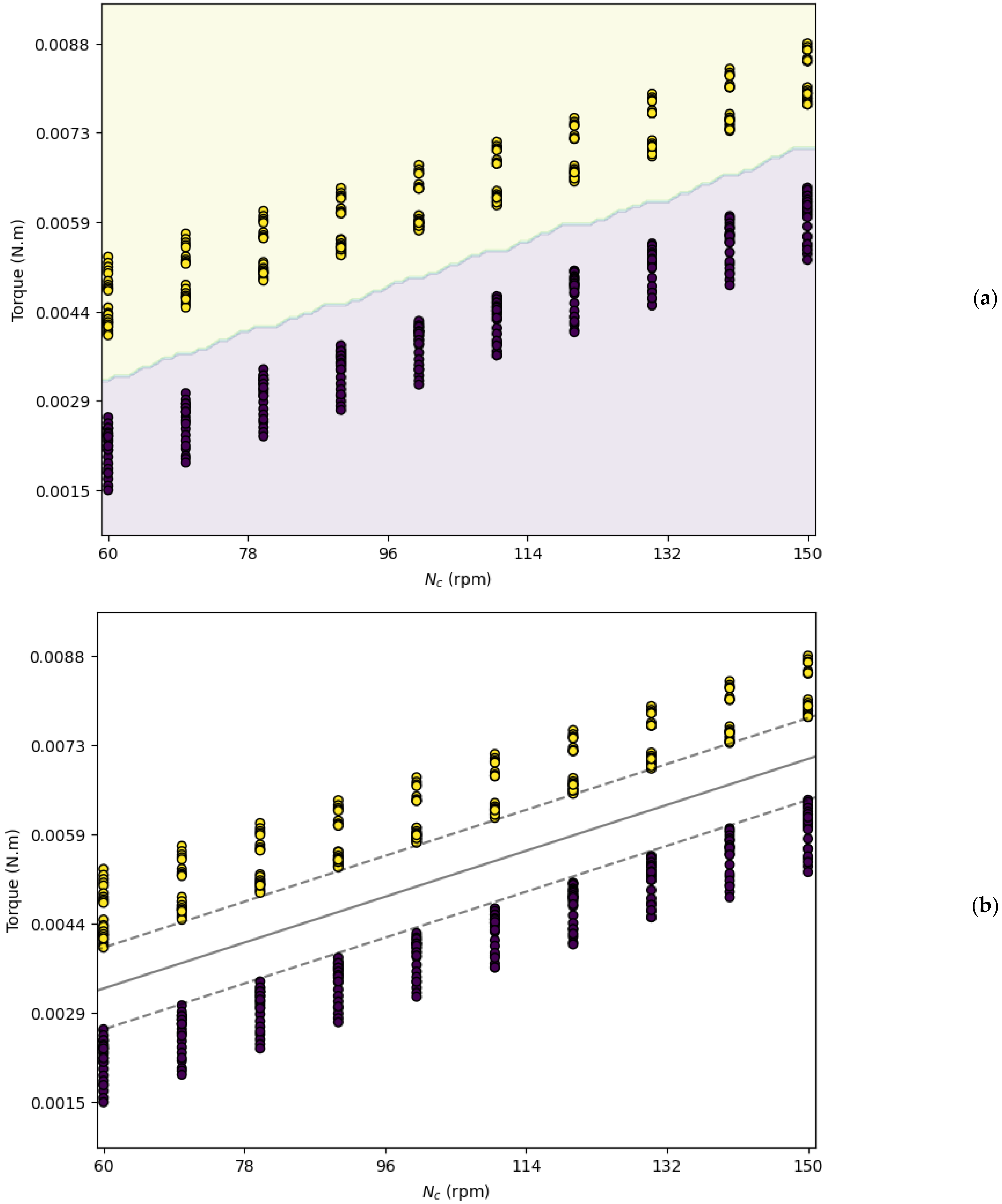
Consequently, a refined classification model was developed by considering only torque and Nc as features. Remarkably, the kNN algorithm, with k set to three, predicted the rotating mode of the coaxial mixer with 100% accuracy using these two features alone. Despite concerns about potential overfitting due to perfect accuracy, the visual analysis in Figure 3 supports the model’s validity. This figure illustrates that the two rotating modes are distinctly separable by the kNN method and shows the importance of feature selection in enhancing model performance. In particular, Figure 3 suggests that a simple linear decision boundary can effectively solve the classification problem, in contrast to the initial model that incorporated all five features but did not achieve perfect prediction.
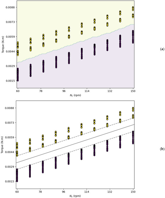
Figure 3.
Decision boundary: (a) kNN model and (b) SVM model (yellow color represents the counter-rotating mode, and purple color represents the co-rotating mode).
The decision boundary obtained by the kNN model is illustrated in Figure 3a. The yellow and purple regions correspond to the counter-rotating and co-rotating modes, respectively, showcasing clear class separation. The efficacy of feature selection and dimensionality reduction was further investigated by employing the SVM model, as depicted in Figure 3b. The SVM’s decision boundary and margin lines are distinctly illustrated. For this SVM model, a linear kernel was employed. The regularization parameter C was set to a very high value (C = 100.0) to ensure a hard margin.
Figure 3b confirms that the SVM model, like the kNN model, accurately predicted the rotating modes. However, a notable distinction lies in their computational efficiency. While the kNN model required storing the entire dataset to classify new instances, the SVM model only relied on the support vectors. This characteristic significantly reduced the SVM model’s memory requirements and computational load compared to those of the kNN model.
This finding holds considerable significance, showing that by considering merely the central impeller speed and the torque value, the rotation mode can be determined. This is particularly relevant in many biochemical applications, where limitations are imposed on the maximum impeller speed and the highest permissible power consumption. Consequently, in these applications, by taking the maximum values for central impeller speed and torque into account, the rotating mode of the coaxial mixer can be strategically determined.
3.2. Regression
In this section of the study, machine learning techniques were employed to predict the torque generated by the coaxial mixer. In fact, the torque values were designated as the response variable, and other operational parameters were considered features. Initially, the MLP method was applied as a regression model. However, the performance of the MLP regressor was found to be unsatisfactory. This necessitated a comprehensive optimization of the MLP’s hyper-parameters to enhance the model’s predictive accuracy.
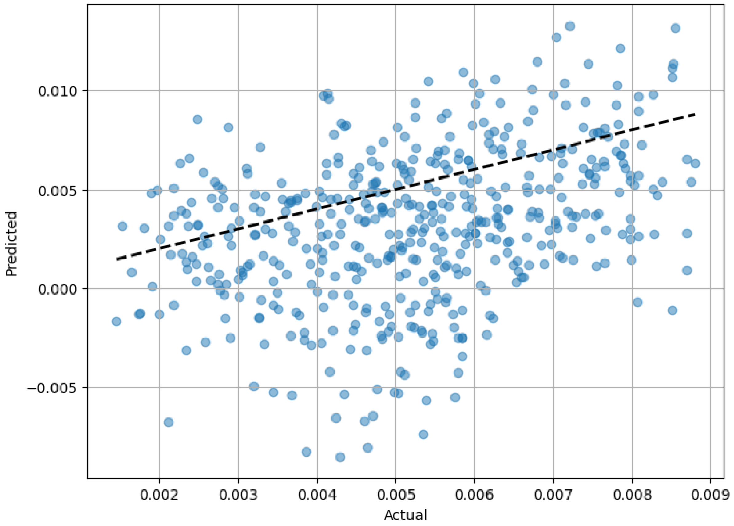
The optimization process was conducted using the GridSearchCV tool from the Scikit-Learn library. The specific parameters and their optimized values used to train the MLP model are detailed in Table 3. Despite these efforts, as depicted in Figure 4, the MLP model struggled to accurately fit the data. This is quantitatively evidenced by a MSE of 1.72 × 10⁻⁵ and an R2 score of −5.52. In fact, a negative R2 is indicative of a model that performed worse than a simplistic model that merely predicts the mean of the target variable for all observations.
Table 3.
Hyper-parameters used to train the MLP regressor.

Figure 4.
Predicted vs. actual torque value obtained from the MLP regressor for the test dataset.
This was due to the fact that the inclusion of the rotating mode as a feature introduced a significant level of complexity to the model. This complexity likely exacerbated the challenges in capturing the underlying patterns of the data and led to the model’s poor performance. The performance of the MLP regressor in terms of the actual vs. predicted torque value based on the test data set is presented in Figure 4. This figure confirms the poor performance of the MLP model.
After the MLP regressor failure to accurately predict the torque generated by the coaxial mixer, the capability of the kNN regressor was investigated as an alternative approach. The kNN regressor functions similarly to its classification counterpart. However, for regression tasks, the predicted value for a new data point is determined based on the average of the values of its k nearest neighbors, rather than voting on the most frequent label.
For this analysis, 70% of the data was allocated for training the kNN regressor. To ensure the robustness of the model, cross-validation was conducted exclusively on the training data. Through a trial-and-error approach, 10-fold cross-validation was identified as sufficient for achieving almost the highest performance.
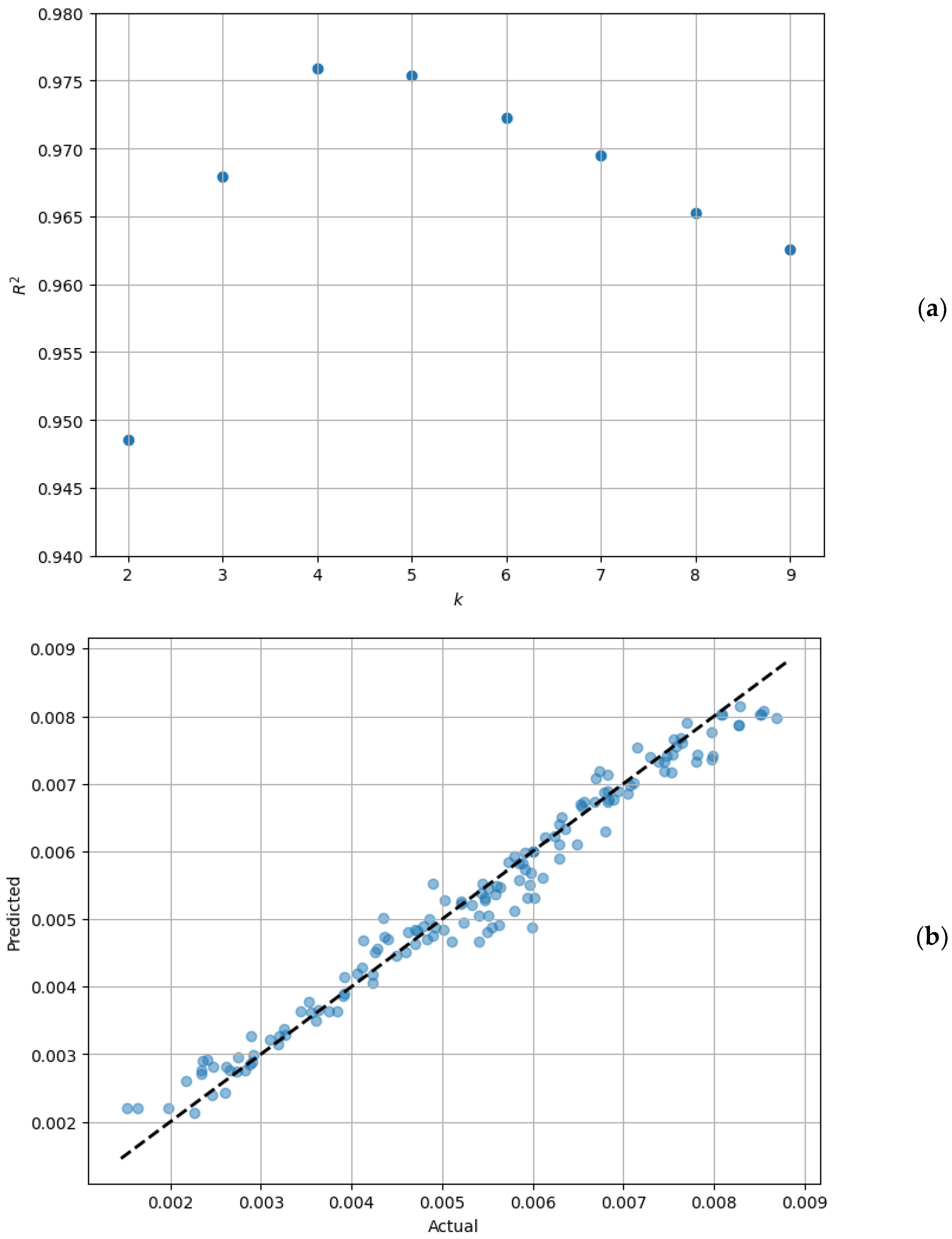
The tuning of the k parameter was performed during the training phase based on the R2 score. As depicted in Figure 5a, the model’s performance peaked at k = 4, achieving an R2 score of 0.976. Consequently, the performance of the kNN regressor was assessed using the unseen test dataset with k set to four. It is noteworthy that the test data were kept entirely separate from the training process, ensuring a rigorous evaluation of the model’s predictive ability.
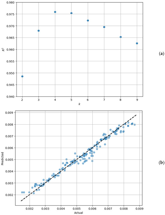
Figure 5.
The performance of the kNN regressor: (a) Tuning the k parameter and (b) predicted vs. actual torque value for the test dataset.
The results obtained from the kNN regressor were promising. The model demonstrated a MSE of 1.006 × 10⁻⁷ and an R2 score of 0.968 on the test data. The concordance between the predicted and actual torque values for the test dataset is depicted in Figure 5b. As can be seen in this figure, the kNN regressor was able to predict the torque with quite reasonable accuracy.
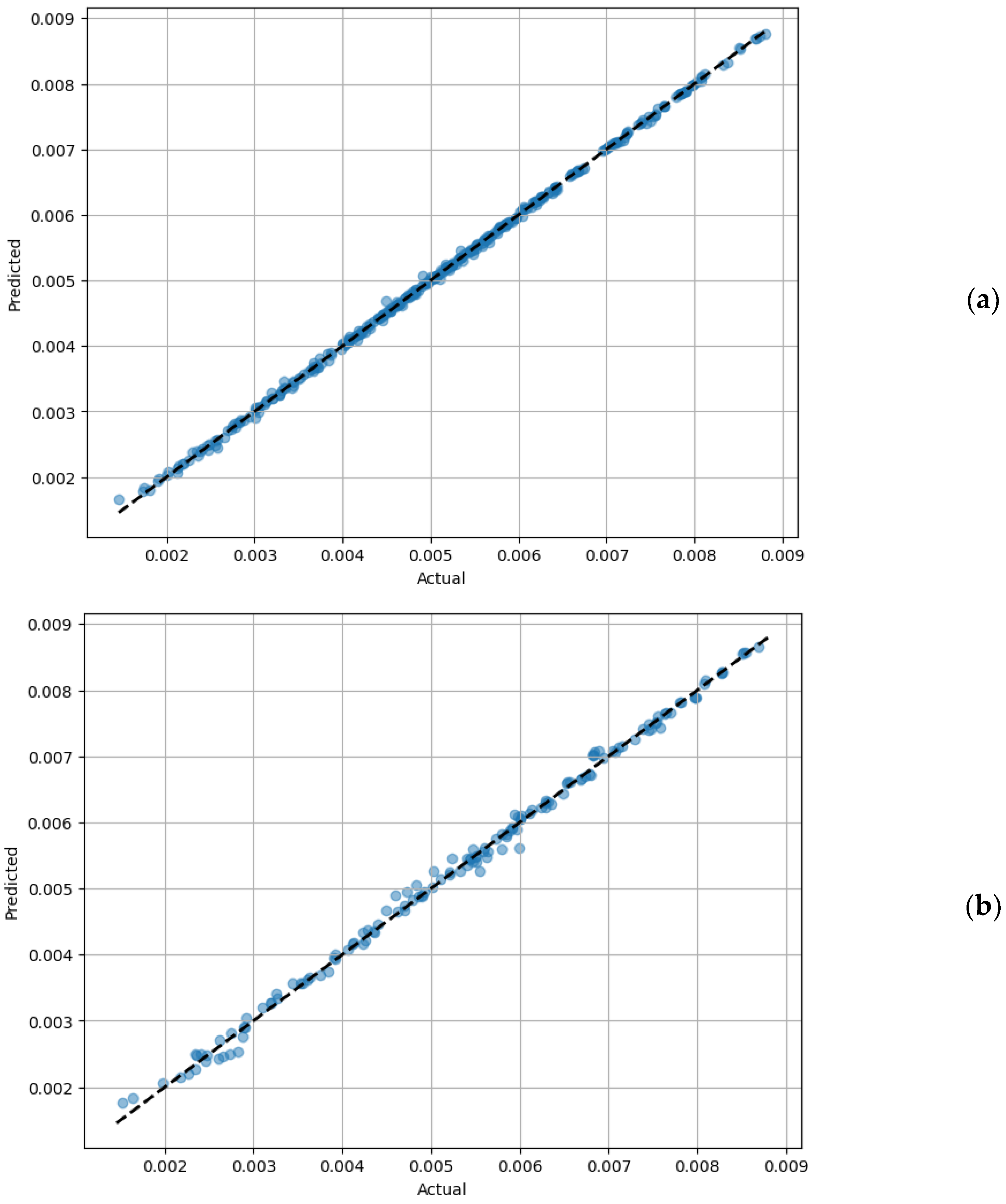
To further enhance the predictive accuracy of the regression model, the random forest regressor was employed. This model was trained using 70% of the data, with the ensemble comprising 100 decision trees referred to as weak learners. The random forest regressor demonstrated exceptional fitting to the training data, with a low MSE of 1.32 × 10⁻⁹ and an R2 score of 0.999 (Figure 6a). This finding indicated that the most effective method for predicting the performance of the coaxial mixer was through the use of ensemble machine learning techniques. This was consistent with the findings of Barros et al. [23], which demonstrated the superiority of stacked neural networks in predicting the mass transfer coefficient over other ANN models.
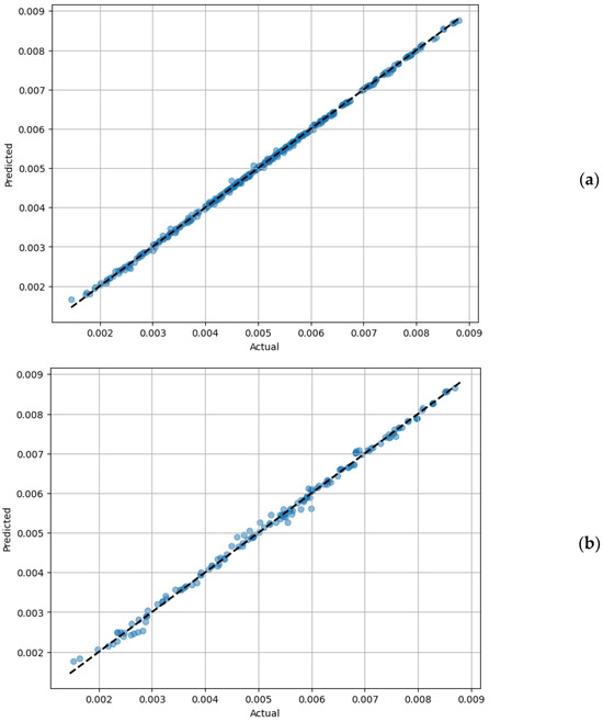

Figure 6.
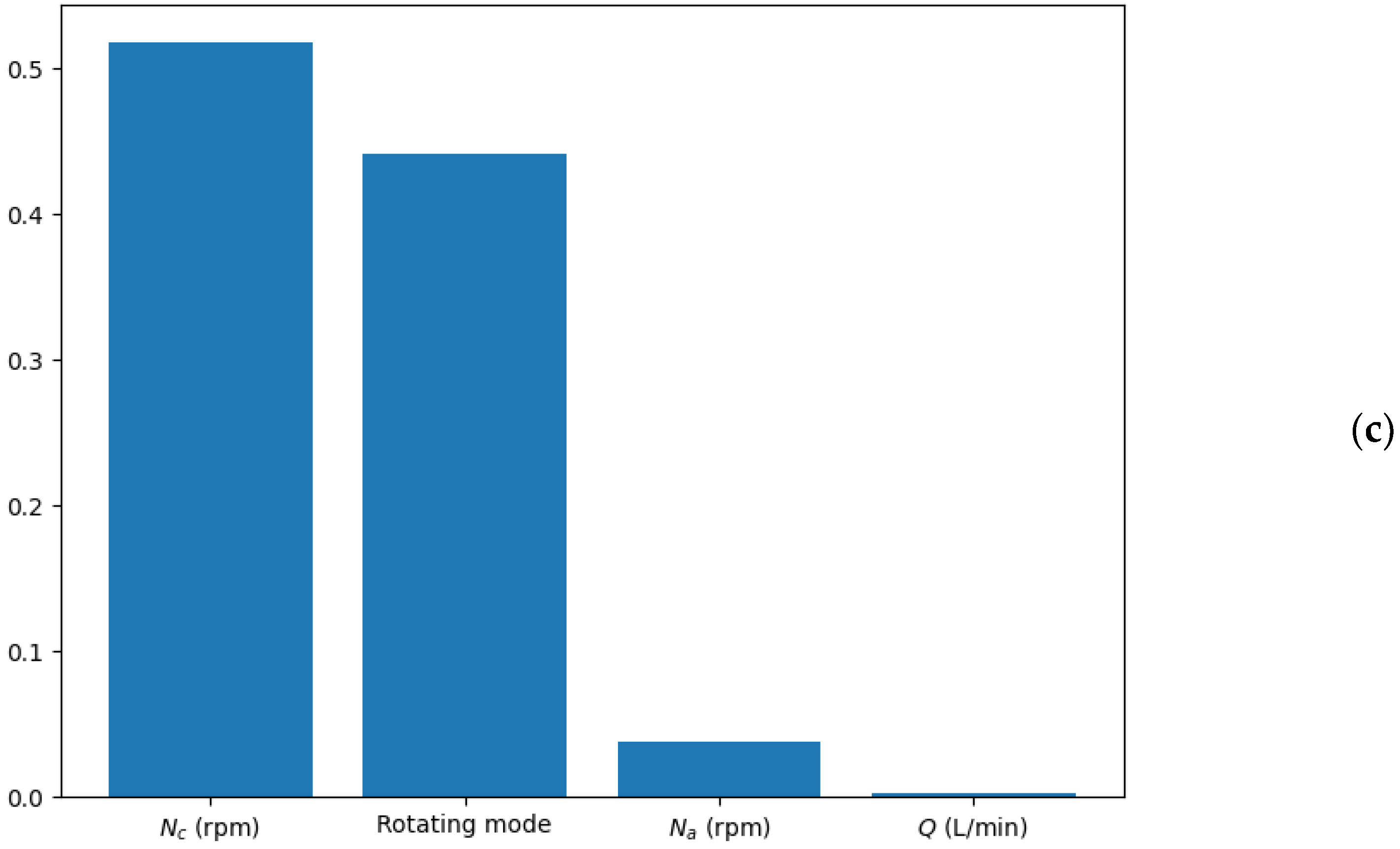
The performance of the random forest regressor. (a) Predicted vs. actual torque value for the training dataset, (b) predicted vs. actual torque value for the test dataset, and (c) feature importance analysis.
The model’s efficacy extended to the test data as well, with performance metrics confirming its robustness (Figure 6b). It was revealed that the MSE and R2 for the test data were 1.07 × 10⁻⁸ and 0.996, respectively. These results underline the model’s capability to generalize well to unseen data. As illustrated in Figure 6b, the congruence between the actual and predicted torque values for the coaxial mixer reinforces the near-perfect prediction accuracy of the random forest regressor.
A noteworthy advantage of the random forest model is its inherent ability to assess the importance of each feature used in the regression. This analysis was conducted based on the Gini gain from the decision trees within the ensemble. As depicted in Figure 6c, it was discerned that the rotating mode was one of the most influential features in determining the torque of the coaxial mixer. This observation is consistent with the patterns illustrated in Figure 3, where the rotating mode was shown to substantially affect the torque value. Therefore, incorporating the rotating mode into the model was pivotal for accurately predicting the torque.
Furthermore, the analysis of feature importance revealed that the central impeller speed was the most significant factor, aligning with previous findings that suggest the central impeller’s primary role in power dissipation within the coaxial bioreactor. Interestingly, the contribution of the aeration rate to the torque of the coaxial mixer was found to be almost negligible.
4. Conclusions
In this study, a coaxial bioreactor equipped with an upward-pumping pitched blade impeller and an anchor impeller containing a non-Newtonian fluid was investigated. A computational fluid dynamics model was developed and validated in terms of power consumption. Then, this numerical model was scaled down by a factor of 0.5. A set of 500 CFD simulations were performed under various operational conditions, including aeration rate (2–6 L/min), central impeller speed (60–150 rpm), anchor impeller speed (3.5–9.5 rpm), and rotating mode (co-rotating and counter-rotating). The torque obtained from the CFD simulations was included in the dataset.
The dataset acquired from the CFD simulations was scaled using the MinMax method. The k-fold cross-validation method was performed on the training dataset to avoid any overfitting problems. In addition, hyperparameter tuning was conducted to enhance the performance of each machine learning model.
The kNN and SVM models were utilized to solve the classification problem. In this problem, the rotating mode of the coaxial bioreactor was successfully labeled based on all feature sets. However, after careful feature selection, the performance of the machine learning classifiers was almost seamless. It was found that the rotating mode of the coaxial bioreactor could be predicted by using only the central impeller speed and the torque of the aerated coaxial mixer. This finding is important, especially where the bioreactor is susceptible to the maximum amount of power dissipation and impeller speed.
In addition, machine learning-based regression models were used to predict the torque produced by the coaxial bioreactor. For the regression problem, the rotating mode was considered a feature, and torque values were set as the target parameter. This regression task was challenging because the torque values were separated based on the rotating mode of the coaxial bioreactor. Different machine learning-based regressors were used, including MLP, kNN, and random forest. The random forest model exhibited promising performance and was able to predict the torque with high accuracy. Notably, the results of the feature importance analysis revealed that the effects of the rotating mode and central impeller speed on the torque of the aerated coaxial mixer were significant.
Author Contributions
Conceptualization, A.R., S.R., F.E.-M. and A.L.; methodology, A.R., F.E.-M. and A.L.; software, A.R. and S.R.; validation, A.R. and S.R.; formal analysis, A.R.; investigation, A.R. and S.R.; resources, F.E.-M. and A.L.; data curation, A.R. and S.R.; writing—original draft preparation, A.R. and S.R.; writing—review and editing, F.E.-M. and A.L.; visualization, A.R.; supervision, F.E.-M. and A.L.; project administration, F.E.-M. and A.L.; funding acquisition, F.E.-M. and A.L. All authors. All authors have read and agreed to the published version of the manuscript.
Funding
Natural Sciences and Engineering Research Council of Canada: RGPIN-2019-04644 and RGPIN-2019-05644.
Data Availability Statement
All of the code program and dataset are available on https://github.com/Ali-Rzadeh/ML-in-coaxial-bioreactor. accessed on 3 March 2024.
Acknowledgments
The financial support of the Natural Sciences and Engineering Research Council of Canada (NSERC) is gratefully acknowledged. CFD simulations were performed on the Niagara supercomputer at the SciNet HPC Consortium. We are deeply grateful to ANSYS for providing us with a high-performance computing license for the ANSYS FLUENT software.
Conflicts of Interest
The authors declare no conflicts of interest.
References
- Petříček, R.; Moucha, T.; Rejl, F.J.; Valenz, L.; Haidl, J.; Čmelíková, T. Volumetric mass transfer coefficient, power input and gas hold-up in viscous liquid in mechanically agitated fermenters. Measurements and scale-up. Int. J. Heat Mass Transf. 2018, 124, 1117–1135. [Google Scholar] [CrossRef]
- Roque, T.; Augier, F.; Hardy, N.; Chaabane, F.B.; Béal, C.; Roque, T.; Augier, F.; Hardy, N.; Chaabane, F.B.; Nienow, A. Mitigation of hydrodynamics related stress in bioreactors: A key for the scale-up of enzyme production by filamentous fungi. In Proceedings of the 16th European Conference on Mixing–Mixing, Birmingham, UK, 9–12 September 2018. [Google Scholar]
- Garcia-Ochoa, F.; Gomez, E. Bioreactor scale-up and oxygen transfer rate in microbial processes: An overview. Biotechnol. Adv. 2009, 27, 153–176. [Google Scholar] [CrossRef] [PubMed]
- Amiraftabi, M.; Khiadani, M.; Mohammed, H.A. Performance of a dual helical ribbon impeller in a two-phase (gas-liquid) stirred tank reactor. Chem. Eng. Process. Process Intensif. 2020, 148, 107811. [Google Scholar] [CrossRef]
- Nienow, A.W.; Bujalski, W. The Versatility of Up-Pumping Hydrofoil Agitators. Chem. Eng. Res. Des. 2004, 82, 1073–1081. [Google Scholar] [CrossRef]
- Paglianti, A.; Takenaka, K.; Bujalski, W. Simple model for power consumption in aerated vessels stirred by Rushton disc turbines. AIChE J. 2001, 47, 2673–2683. [Google Scholar] [CrossRef]
- McFarlane, C.M.; Zhao, X.-M.; Nienow, A.W. Studies of high solidity ratio hydrofoil impellers for aerated bioreactors. 2. Air-water studies. Biotechnol. Prog. 1995, 11, 608–618. [Google Scholar] [CrossRef]
- Nienow, A.W. Hydrodynamics of Stirred Bioreactors. Appl. Mech. Rev. 1998, 51, 3–32. [Google Scholar] [CrossRef]
- Aubin, J.; Mavros, P.; Fletcher, D.F.; Bertrand, J.; Xuereb, C. Effect of Axial Agitator Configuration (Up-Pumping, Down-Pumping, Reverse Rotation) on Flow Patterns Generated in Stirred Vessels. Chem. Eng. Res. Des. 2001, 79, 845–856. [Google Scholar] [CrossRef]
- Vrábel, P.; van der Lans, R.G.J.M.J.M.; Luyben, K.C.A.A.M.; Boon, L.; Nienow, A.W. Mixing in large-scale vessels stirred with multiple radial or radial and axial up-pumping impellers: Modelling and measurements. Chem. Eng. Sci. 2000, 55, 5881–5896. [Google Scholar] [CrossRef]
- Vilaça, P.R.; Badino, A.C.; Facciotti, M.C.R.; Schmidell, W. Determination of power consumption and volumetric oxygen transfer coefficient in bioreactors. Bioprocess Eng. 2000, 22, 261–265. [Google Scholar] [CrossRef]
- Bouaifi, M.; Roustan, M. Power consumption, mixing time and homogenisation energy in dual-impeller agitated gas–liquid reactors. Chem. Eng. Process. Process Intensif. 2001, 40, 87–95. [Google Scholar] [CrossRef]
- Doran, P. Bioprocess Engineering Principles, 2nd ed.; Elsevier: Amsterdam, The Netherlands, 2013. [Google Scholar] [CrossRef]
- Taghavi, M.; Zadghaffari, R.; Moghaddas, J.; Moghaddas, Y. Experimental and CFD investigation of power consumption in a dual Rushton turbine stirred tank. Chem. Eng. Res. Des. 2011, 89, 280–290. [Google Scholar] [CrossRef]
- Rahimzadeh, A.; Ein-mozaffari, F.; Lohi, A. A Methodical Approach to Scaling Up an Aerated Coaxial Mixer Containing a Shear-Thinning Fluid: Effect of the Fluid Rheology. Ind. Eng. Chem. Res. 2023, 62, 8454–8476. [Google Scholar] [CrossRef]
- Rahimzadeh, A.; Ein-mozaffari, F.; Lohi, A. Development of a scale-up strategy for an aerated coaxial mixer containing a non-Newtonian fluid: A mass transfer approach. Phys. Fluids 2023, 35, 073103. [Google Scholar] [CrossRef]
- Rahimzadeh, A.; Ein-mozaffari, F.; Lohi, A. Investigation of power consumption, torque fluctuation, and local gas hold-up in coaxial mixers containing a shear-thinning fluid: Experimental and numerical approaches. Chem. Eng. Process. Process Intensif. 2022, 177, 108983. [Google Scholar] [CrossRef]
- Liu, B.; Huang, B.; Zhang, Y.; Liu, J.; Jin, Z. Numerical study on gas dispersion characteristics of a coaxial mixer with viscous fluids. J. Taiwan Inst. Chem. Eng. 2016, 66, 54–61. [Google Scholar] [CrossRef]
- Barros, P.L.; Ein-Mozaffari, F.; Lohi, A. Power Consumption Characterization of Energy-Efficient Aerated Coaxial Mixers Containing Yield-Stress Biopolymer Solutions. Ind. Eng. Chem. Res. 2022, 61, 12813–12824. [Google Scholar] [CrossRef]
- Sharifi, F.; Behzadfar, E.; Ein-Mozaffari, F. Investigating the power consumption for the intensification of gas dispersion in a dual coaxial mixer containing yield-pseudoplastic fluids. Chem. Eng. Process. Process Intensif. 2023, 191, 109461. [Google Scholar] [CrossRef]
- Bowler, A.L.; Bakalis, S.; Watson, N.J. Monitoring Mixing Processes Using Ultrasonic Sensors and Machine Learning Alexander. Sensor 2020, 20, 1813. [Google Scholar] [CrossRef]
- Kumar, P.; Sinha, K.; Nere, N.K.; Shin, Y.; Ho, R.; Mlinar, L.B.; Sheikh, A.Y. A machine learning framework for computationally expensive transient models. Sci. Rep. 2020, 10, 11492. [Google Scholar] [CrossRef]
- Barros, P.L.; Ein-Mozaffari, F.; Lohi, A.; Upreti, S. Exploiting the prediction of mass transfer performance in aerated coaxial mixers containing biopolymer solutions using empirical correlations and neural networks. Can. J. Chem. Eng. 2023, 1–18. [Google Scholar] [CrossRef]
- Yang, C.; Yao, J.; Chen, X.; Xie, M.; Zhou, G.; Xu, Z.; Liu, B. Chemical Engineering Research and Design Experimental study on gas-liquid flow regimes of coaxial mixers equipped with a Rushton/pitched blade turbine and anchor. Chem. Eng. Res. Des. 2024, 202, 377–389. [Google Scholar] [CrossRef]
- Bibeau, V.; Barbeau, L.; Boffito, D.C.; Blais, B. Artificial neural network to predict the power number of agitated tanks fed by CFD simulations. Can. J. Chem. Eng. 2023, 101, 5992–6002. [Google Scholar] [CrossRef]
- Chen, M.; Wang, J.; Zhao, S.; Xu, C.; Feng, L. Optimization of Dual-Impeller Configurations in a Gas-Liquid Stirred Tank Based on Computational Fluid Dynamics and Multiobjective Evolutionary Algorithm. Ind. Eng. Chem. Res. 2016, 55, 9054–9063. [Google Scholar] [CrossRef]
- Kang, Z.; Feng, L.; Wang, J. Optimization of a Gas–Liquid Dual-Impeller Stirred Tank Based on Deep Learning with a Small Data Set from CFD Simulation. Ind. Eng. Chem. Res. 2023, 63, 843–855. [Google Scholar] [CrossRef]
- Laubscher, R.; Rousseau, P. Application of generative deep learning to predict temperature, flow and species distributions using simulation data of a methane combustor. Int. J. Heat Mass Transf. 2020, 163, 120417. [Google Scholar] [CrossRef]
- Taira, K.; McInnes, D.; Zhang, L. How many data points and how large an R-squared value is essential for Arrhenius plots? J. Catal. 2023, 419, 26–36. [Google Scholar] [CrossRef]
- Liu, Y.; Li, C.; Bao, J.; Wang, X.; Yu, W.; Shao, L. Degradation of Azo Dyes with Different Functional Groups in Simulated Wastewater by Electrocoagulation. Water 2022, 14, 123. [Google Scholar] [CrossRef]
- Kathamuthu, N.D.; Subramaniam, S.; Le, Q.H.; Muthusamy, S.; Panchal, H.; Sundararajan, S.C.M.; Alrubaie, A.J.; Zahra, M.M.A. A deep transfer learning-based convolution neural network model for COVID-19 detection using computed tomography scan images for medical applications. Adv. Eng. Softw. 2023, 175, 103317. [Google Scholar] [CrossRef]
- Mu’azu, N.D.; Olatunji, S.O. K-nearest neighbor based computational intelligence and RSM predictive models for extraction of Cadmium from contaminated soil. Ain Shams Eng. J. 2023, 14, 101944. [Google Scholar] [CrossRef]
- Briceno-Mena, L.A.; Arges, C.G.; Romagnoli, J.A. Machine learning-based surrogate models and transfer learning for derivative free optimization of HT-PEM fuel cells. Comput. Chem. Eng. 2023, 171, 108159. [Google Scholar] [CrossRef]
- Houssein, E.H.; Hosney, M.E.; Oliva, D.; Mohamed, W.M.; Hassaballah, M. A novel hybrid Harris hawks optimization and support vector machines for drug design and discovery. Comput. Chem. Eng. 2020, 133, 106656. [Google Scholar] [CrossRef]
- Mir, A.; Nasiri, J.A. KNN-based least squares twin support vector machine for pattern classification. Appl. Intell. 2018, 48, 4551–4564. [Google Scholar] [CrossRef]
- Tang, L.; Tian, Y.; Yang, C. Nonparallel support vector regression model and its SMO-type solver. Neural Netw. 2018, 105, 431–446. [Google Scholar] [CrossRef] [PubMed]
- Liu, J.; Zhang, Z.; Li, X.; Zong, M.; Wang, Y.; Wang, S.; Chen, P.; Wan, Z.; Liu, L.; Liang, Y.; et al. Machine learning assisted phase and size-controlled synthesis of iron oxide particles. Chem. Eng. J. 2023, 473, 145216. [Google Scholar] [CrossRef]
- Zhao, S.; Guo, J.; Dang, X.; Ai, B.; Zhang, M.; Li, W.; Zhang, J. Energy consumption, flow characteristics and energy-efficient design of cup-shape blade stirred tank reactors: Computational fluid dynamics and artificial neural network investigation. Energy 2022, 240, 122474. [Google Scholar] [CrossRef]
- Frontistis, Z.; Lykogiannis, G.; Sarmpanis, A. Machine Learning Implementation in Membrane Bioreactor Systems: Progress, Challenges, and Future Perspectives: A Review. Environments 2023, 10, 127. [Google Scholar] [CrossRef]
- Wang, T.; Li, Y.Y. Predictive modeling based on artificial neural networks for membrane fouling in a large pilot-scale anaerobic membrane bioreactor for treating real municipal wastewater. Sci. Total Environ. 2024, 912, 169164. [Google Scholar] [CrossRef] [PubMed]
- Zaghloul, M.S.; Iorhemen, O.T.; Hamza, R.A.; Tay, J.H.; Achari, G. Development of an ensemble of machine learning algorithms to model aerobic granular sludge reactors. Water Res. 2021, 189, 116657. [Google Scholar] [CrossRef]
- Rajković, D.; Jeromela, A.M.; Pezo, L.; Lončar, B.; Grahovac, N.; Špika, A.K. Artificial neural network and random forest regression models for modelling fatty acid and tocopherol content in oil of winter rapeseed. J. Food Compos. Anal. 2023, 115, 105020. [Google Scholar] [CrossRef]
- Yan, B.; Jiang, L.; Zhou, H.; Atakpa, E.O.; Bo, K.; Li, P.; Xie, Q.; Li, Y.; Zhang, C. Performance and microbial community analysis of combined bioreactors in treating high–salinity hydraulic fracturing flowback and produced water. Bioresour. Technol. 2023, 386, 129469. [Google Scholar] [CrossRef] [PubMed]
Disclaimer/Publisher’s Note: The statements, opinions and data contained in all publications are solely those of the individual author(s) and contributor(s) and not of MDPI and/or the editor(s). MDPI and/or the editor(s) disclaim responsibility for any injury to people or property resulting from any ideas, methods, instructions or products referred to in the content. |
© 2024 by the authors. Licensee MDPI, Basel, Switzerland. This article is an open access article distributed under the terms and conditions of the Creative Commons Attribution (CC BY) license (https://creativecommons.org/licenses/by/4.0/).