
Adaptive Filtering with Fitted Noise Estimate (AFFiNE): Blink Artifact Correction in Simulated and Real P300 Data


Abstract
:
1. Introduction
2. Materials and Methods
2.1. EEG Recording
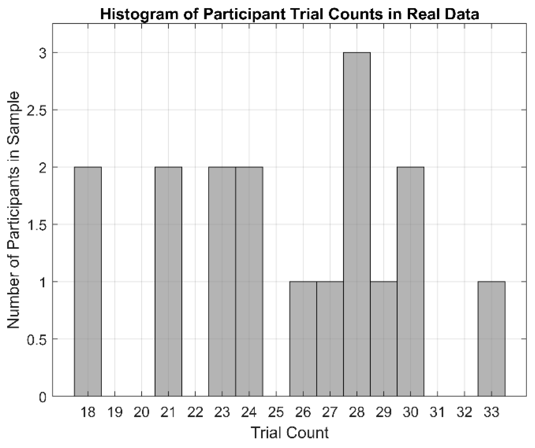
2.1.1. Participants
2.1.2. Stimuli and P300 Task
2.1.3. Recording Equipment
2.2. EEG Simulation
2.2.1. Task-Irrelevant EEG: Noise Signal
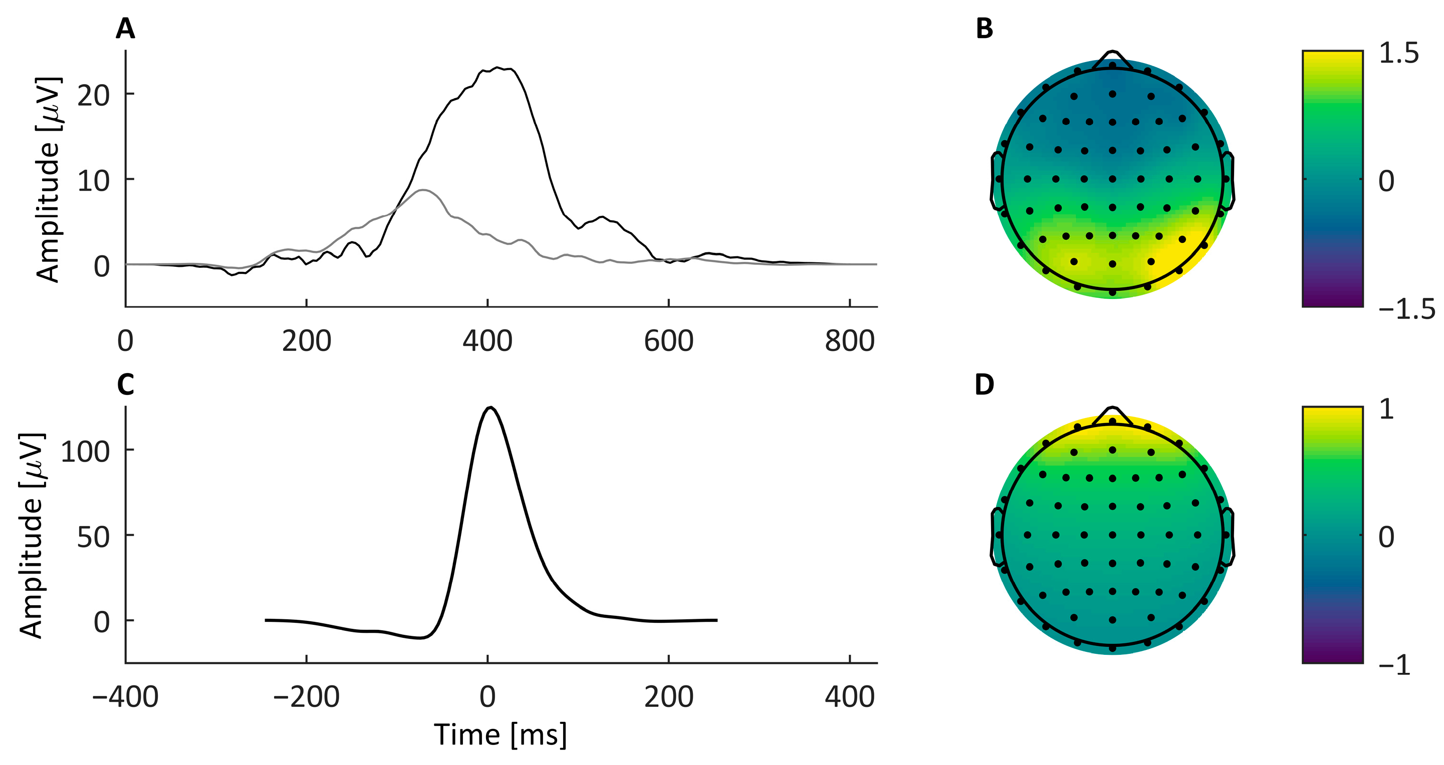
2.2.2. Task-Relevant EEG: ERP Signal
2.2.3. Artifact-Relevant EEG: Blink Signal
2.2.4. Creating Simulated Timeseries Data
2.3. Data Analysis
2.3.1. Pre-Processing
2.3.2. Artifact Correction Methods
2.3.3. Epoch Sorting by Artifact
2.3.4. ERP Waveforms and Topographical Errors
2.3.5. P300 Measurements
2.4. Statistical Analysis
3. Results
3.1. Simulated Data Results
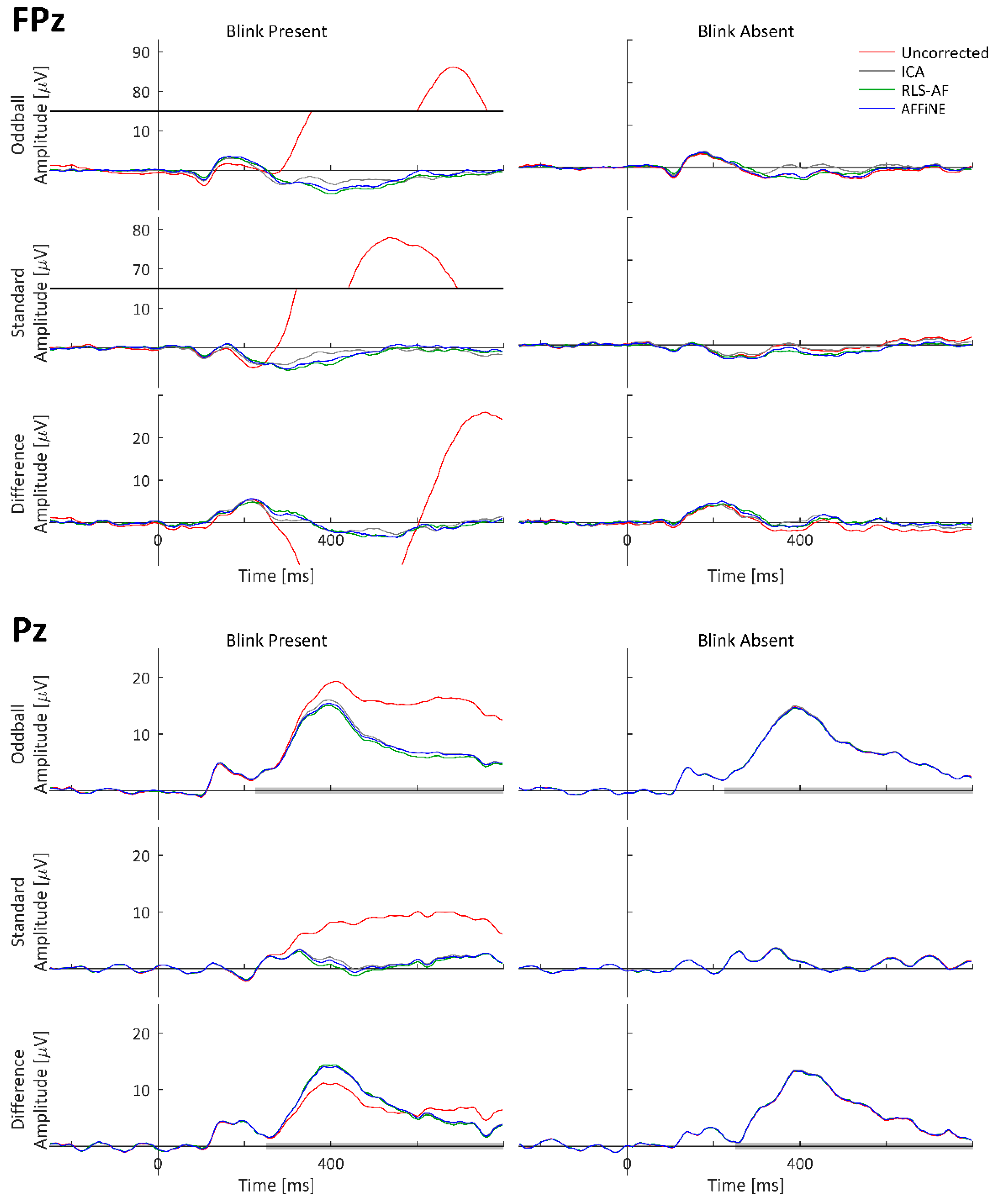
3.1.1. ERP Waveforms
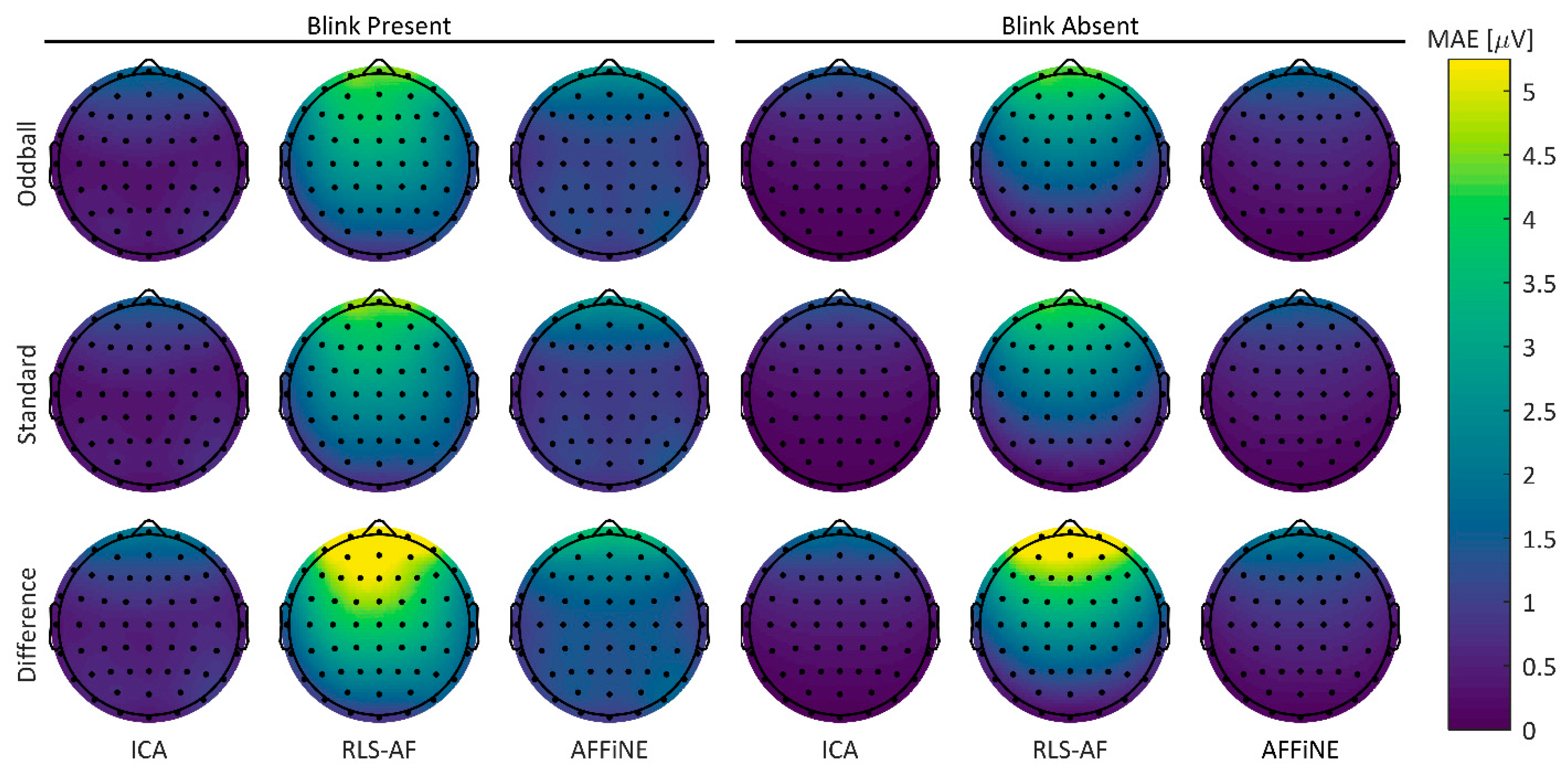
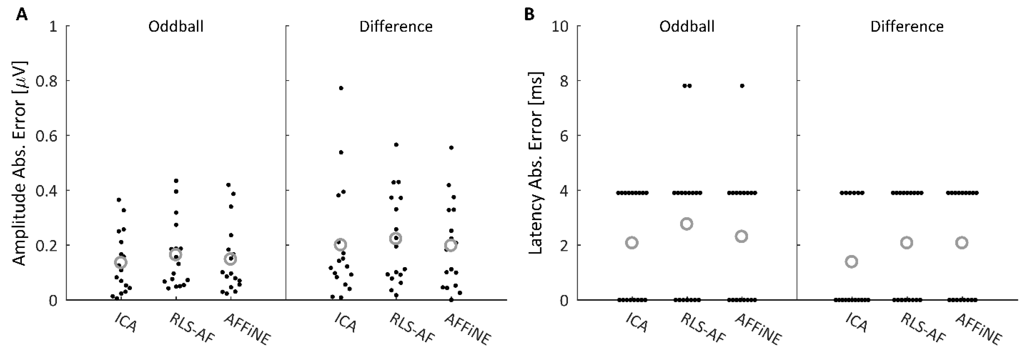
3.1.2. Topographical Errors
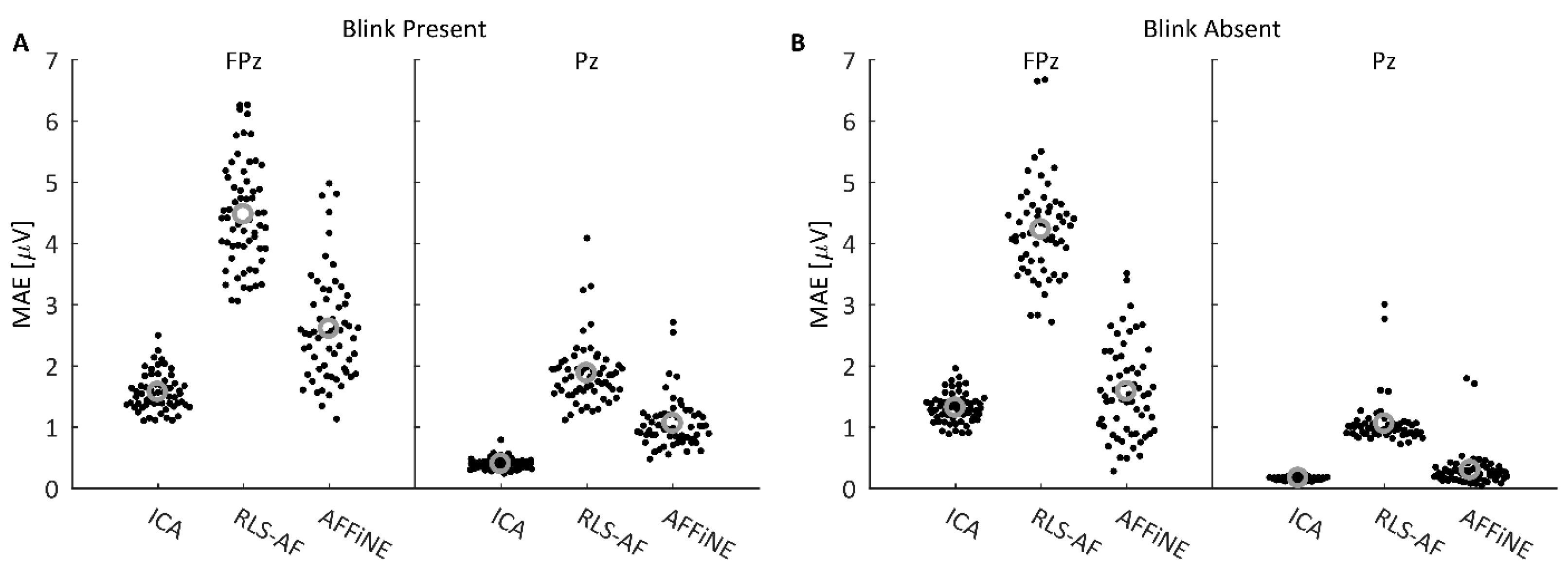
3.1.3. Analysis at FPz and Pz
3.2. Real Data Results
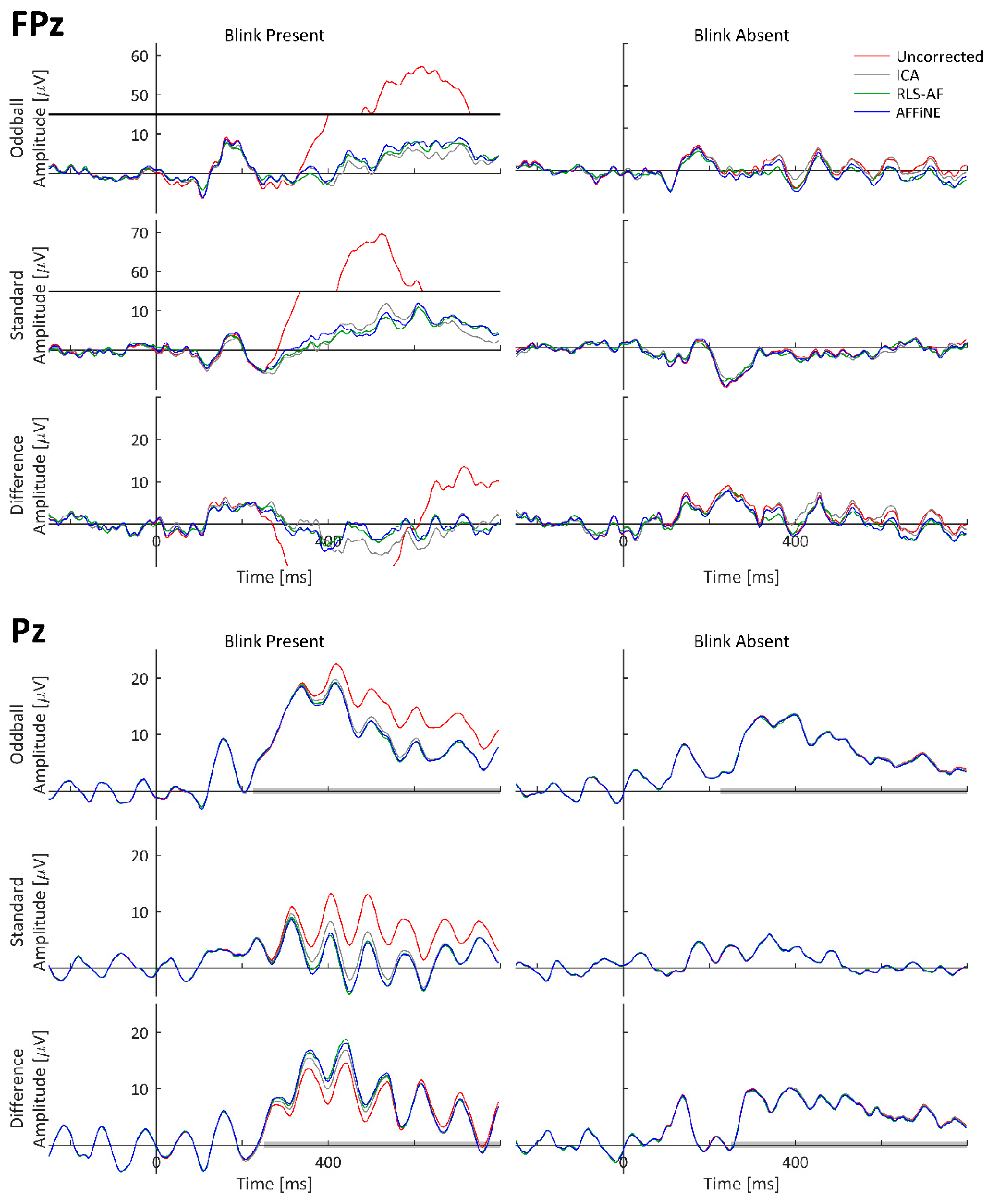
3.2.1. ERP Waveforms
3.2.2. Topographical Errors
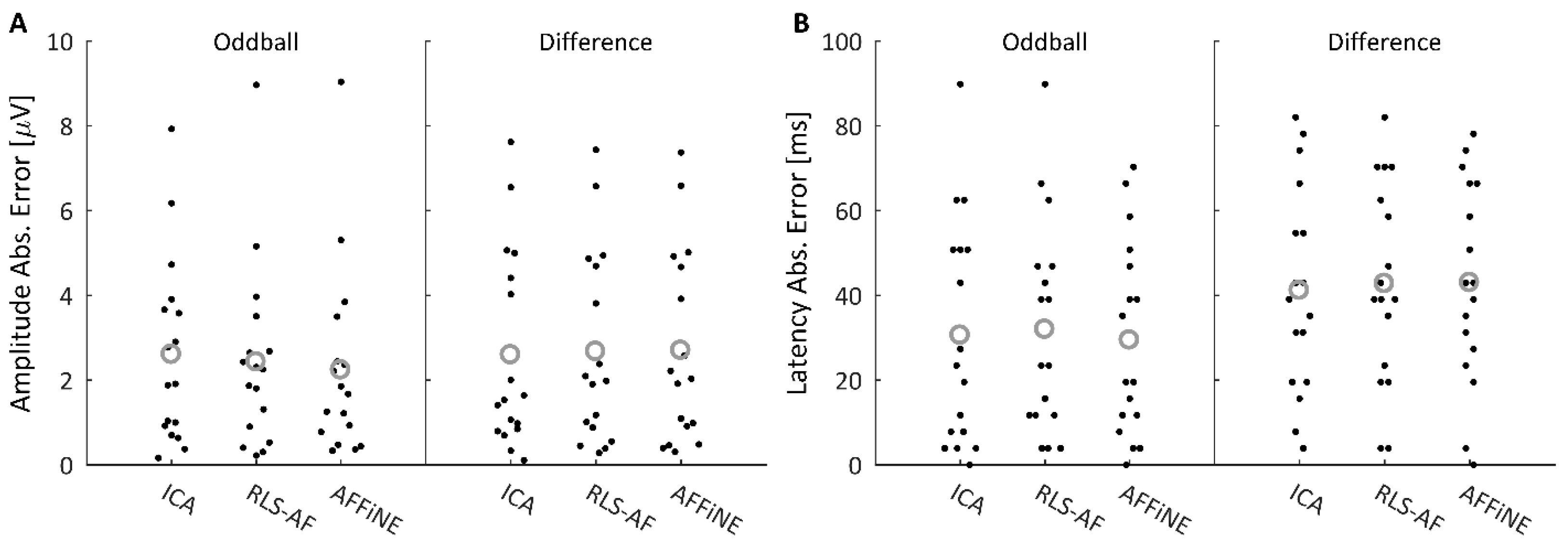
3.2.3. Measurement Errors in the Blink Absent Condition
3.2.4. Measurement Errors in the Blink Present Condition
4. Discussion
4.1. Simulated Data Results
4.2. Real Data Results
4.3. Algorithm Performance Comparison in Simulated vs. Real Data
4.4. Differences between Simulated and Real Data
4.5. Extension of AFFiNE to Other Artifact Types
5. Conclusions
Author Contributions
Funding
Institutional Review Board Statement
Informed Consent Statement
Data Availability Statement
Acknowledgments
Conflicts of Interest
Disclaimer/Authors’ Note
References
- Luck, S.J. An Introduction to the Event-Related Potential Techniques; The MIT Press: Cambridge, MA, USA, 2005; ISBN 9780262525855. [Google Scholar]
- Hillyard, S.A.; Galambos, R. Eye Movement Artifact in the CNV. Electroencephalogr. Clin. Neurophysiol. 1970, 28, 173–182. [Google Scholar] [CrossRef]
- Girton, D.G.; Kamiya, J. A Simple On-Line Technique for Removing Eye Movement Artifacts from the EEG. Electroencephalogr. Clin. Neurophysiol. 1973, 34, 212–216. [Google Scholar] [CrossRef]
- Verleger, R.; Gasser, T.; Möcks, J. Correction of EOG Artifacts in Event-Related Potentials of the EEG: Aspects of Reliability and Validity. Psychophysiology 1982, 19, 472–480. [Google Scholar] [CrossRef]
- Croft, R.J.; Barry, R.J. Removal of Ocular Artifact from the EEG: A Review. Neurophysiol. Clin. 2000, 30, 5–19. [Google Scholar] [CrossRef]
- Berg, P.; Scherg, M. A Multiple Source Approach to the Correction of Eye Artifacts. Electroencephalogr. Clin. Neurophysiol. 1994, 90, 229–241. [Google Scholar] [CrossRef]
- Makeig, S.; Bell, A.J.; Jung, T.-P.; Sejnowski, T.J. Independent Component Analysis of Electroencephalographic Data. Adv. Neural Inf. Process Syst. 1996, 8, 145–151. [Google Scholar]
- Mullen, T.R.; Kothe, C.A.E.; Chi, Y.M.; Ojeda, A.; Kerth, T.; Makeig, S.; Jung, T.-P.; Cauwenberghs, G. Real-Time Neuroimaging and Cognitive Monitoring Using Wearable Dry EEG. IEEE Trans. Biomed. Eng. 2015, 62, 2553–2567. [Google Scholar] [CrossRef]
- Pion-Tonachini, L.; Kreutz-Delgado, K.; Makeig, S. ICLabel: An Automated Electroencephalographic Independent Component Classifier, Dataset, and Website. Neuroimage 2019, 198, 181–197. [Google Scholar] [CrossRef]
- Onton, J.; Westerfield, M.; Townsend, J.; Makeig, S. Imaging Human EEG Dynamics Using Independent Component Analysis. Neurosci. Biobehav. Rev. 2006, 30, 808–822. [Google Scholar] [CrossRef]
- He, P.; Wilson, G.; Russell, C. Removal of Ocular Artifacts from Electro-Encephalogram by Adaptive Filtering. Med. Biol. Eng. Comput. 2004, 42, 407–412. [Google Scholar] [CrossRef]
- He, P.; Wilson, G.; Russell, C.; Gerschutz, M. Removal of Ocular Artifacts from the EEG: A Comparison between Time-Domain Regression Method and Adaptive Filtering Method Using Simulated Data. Med. Biol. Eng. Comput. 2007, 45, 495–503. [Google Scholar] [CrossRef]
- Romero, S.; Mañanas, M.A.; Barbanoj, M.J. Ocular Reduction in EEG Signals Based on Adaptive Filtering, Regression and Blind Source Separation. Ann. Biomed. Eng. 2009, 37, 176–191. [Google Scholar] [CrossRef]
- Dimatteo, I.; Genovese, C.R.; Kass, R.E. Bayesian Curve-Fitting with Free-Knot Splines. Biometrika 2001, 88, 1055–1071. [Google Scholar] [CrossRef]
- Wallstrom, G.; Liebner, J.; Kass, R.E. An Implementation of Bayesian Adaptive Regression Splines (BARS) in C with S and R Wrappers. J. Stat. Softw. 2008, 26, 1–21. [Google Scholar] [CrossRef]
- Wolpaw, J.; Wolpaw, E.W. Brain–Computer InterfacesPrinciples and Practice; Oxford University Press: Oxford, UK, 2012; ISBN 9780195388855. [Google Scholar]
- Heidari, S.; Babor, T.F.; De Castro, P.; Tort, S.; Curno, M. Sex and Gender Equity in Research: Rationale for the SAGER Guidelines and Recommended Use. Res. Integr. Peer Rev. 2016, 1, 2. [Google Scholar] [CrossRef]
- Tsolaki, A.; Kosmidou, V.; Hadjileontiadis, L.; Kompatsiaris, I.Y.; Tsolaki, M. Brain Source Localization of MMN, P300 and N400: Aging and Gender Differences. Brain Res. 2015, 1603, 32–49. [Google Scholar] [CrossRef]
- Steffensen, S.C.; Ohran, A.J.; Shipp, D.N.; Hales, K.; Stobbs, S.H.; Fleming, D.E. Gender-Selective Effects of the P300 and N400 Components of the Visual Evoked Potential. Vision Res. 2008, 48, 917–925. [Google Scholar] [CrossRef]
- Fabiani, M.; Karis, D.; Donchin, E. P300 and Recall in an Incidental Memory Paradigm. Psychophysiology 1986, 23, 298–308. [Google Scholar] [CrossRef]
- Fabiani, M.; Gratton, G.; Karis, D.; Donchin, E. Definition, Identification and Reliability of the P300 Component of the Event-Related Brain Potential; JAI Press, Inc.: Stamford, CT, USA, 1987; Volume 2, ISBN 0892326441. [Google Scholar]
- American Electroencephalographic Society. Guideline Thirteen: Guidelines for Standard Electrode Position Nomenclature. J. Clin. Neurophysiol. 1994, 11, 111–113. [Google Scholar] [CrossRef]
- Seeck, M.; Koessler, L.; Bast, T.; Leijten, F.; Michel, C.; Baumgartner, C.; He, B.; Beniczky, S. The Standardized EEG Electrode Array of the IFCN. Clin. Neurophysiol. 2017, 128, 2070–2077. [Google Scholar] [CrossRef]
- Berg, P.; Scherg, M. A Fast Method for Forward Computation of Multiple-Shell Spherical Head Models. Electroencephalogr. Clin. Neurophysiol. 1994, 90, 58–64. [Google Scholar] [CrossRef]
- de Cheveigné, A.; Nelken, I. Filters: When, Why, and How (Not) to Use Them. Neuron 2019, 102, 280–293. [Google Scholar] [CrossRef]
- Lee, T.-W.; Girolami, M.; Sejnowski, T.J. Independent Component Analysis Using an Extended Infomax Algorithm for Mixed Subgaussian and Supergaussian Sources. Neural Comput. 1999, 11, 417–441. [Google Scholar] [CrossRef]
- Delorme, A.; Makeig, S. EEGLAB: An Open Sorce Toolbox for Analysis of Single-Trail EEG Dynamics Including Independent Component Anlaysis. J. Neurosci. Methods 2004, 134, 9–21. [Google Scholar] [CrossRef]
- Iwasaki, M.; Kellinghaus, C.; Alexopoulos, A.V.; Burgess, R.C.; Kumar, A.N.; Han, Y.H.; Lüders, H.O.; Leigh, R.J. Effects of Eyelid Closure, Blinks, and Eye Movements on the Electroencephalogram. Clin. Neurophysiol. 2005, 116, 878–885. [Google Scholar] [CrossRef]
- Lopez-Calderon, J.; Luck, S.J. ERPLAB: An Open-Source Toolbox for the Analysis of Event-Related Potentials. Front. Hum. Neurosci. 2014, 8, 213. [Google Scholar] [CrossRef]
- Gustafsson, F. Determining the Initial States in Forward-Backward Filtering. IEEE Trans. Signal Process. 1996, 44, 988–992. [Google Scholar] [CrossRef]
- Tanner, D.; Morgan-Short, K.; Luck, S.J. How Inappropriate High-Pass Filters Can Produce Artifactual Effects and Incorrect Conclusions in ERP Studies of Language and Cognition. Psychophysiology 2015, 52, 997–1009. [Google Scholar] [CrossRef]
- Winkler, I.; Debener, S.; Müller, K.-R.; Tangermann, M. On the Influence of High-Pass Filtering on ICA-Based Artifact Reduction in EEG-ERP. Annu. Int. Conf. IEEE Eng. Med. Biol. Soc. 2015, 2015, 4101–4105. [Google Scholar] [CrossRef]
- Wallstrom, G.L.; Kass, R.E.; Miller, A.; Cohn, J.F.; Fox, N.A. Automatic Correction of Ocular Artifacts in the EEG: A Comparison of Regression-Based and Component-Based Methods. Int. J. Psychophysiol. 2004, 53, 105–119. [Google Scholar] [CrossRef]
- Wallstrom, G.L.; Kass, R.E.; Miller, A.; Cohn, J.F.; Fox, N.A. Correction of Ocular Artifacts in the EEG Using Bayesian Adaptive Regression Splines; Springer: New York, NY, USA, 2002; pp. 351–365. [Google Scholar]
- Hunter, J.D. Matplotlib: A 2D Graphics Environment. Comput. Sci. Eng. 2007, 9, 90–95. [Google Scholar] [CrossRef]
- Luck, S.J.; Gaspelin, N. How to Get Statistically Significant Effects in Any ERP Experiment (and Why You Shouldn’t). Psychophysiology 2017, 54, 146–157. [Google Scholar] [CrossRef]
- Whitham, E.M.; Pope, K.J.; Fitzgibbon, S.P.; Lewis, T.; Clark, C.R.; Loveless, S.; Broberg, M.; Wallace, A.; DeLosAngeles, D.; Lillie, P.; et al. Scalp Electrical Recording during Paralysis: Quantitative Evidence That EEG Frequencies above 20 Hz Are Contaminated by EMG. Clin. Neurophysiol. 2007, 118, 1877–1888. [Google Scholar] [CrossRef]


| Artifact Condition | Electrode | Test Pairs | M | SD | Statistic | p | |
|---|---|---|---|---|---|---|---|
| Blink Present | FPz | ICA–RLS-AF | −2.901 μV | 0.887 μV | t(59) = −25.323 | <0.001 | * |
| ICA–AFFiNE | −1.033 μV | 0.956 μV | t(59) = −8.372 | <0.001 | * | ||
| RLS-AF–AFFiNE | 1.868 μV | 0.669 μV | t(59) = 21.621 | <0.001 | * | ||
| Pz | ICA–RLS-AF | −1.479 μV | 0.491 μV | t(59) = −23.353 | <0.001 | * | |
| ICA–AFFiNE | −0.658 μV | 0.383 μV | t(59) = −13.329 | <0.001 | * | ||
| RLS-AF–AFFiNE | 0.821 μV | 0.247 μV | t(59) = 25.79 | <0.001 | * | ||
| Blink Absent | FPz | ICA–RLS-AF | −2.912 μV | 0.758 μV | t(59) = −29.737 | <0.001 | * |
| ICA–AFFiNE | −0.265 μV | 0.690 μV | t(59) = −2.977 | 0.004 | * | ||
| RLS-AF–AFFiNE | 2.646 μV | 0.872 μV | t(59) = 23.504 | <0.001 | * | ||
| Pz | ICA–RLS-AF | −0.889 μV | 0.378 μV | t(59) = −18.209 | <0.001 | * | |
| ICA–AFFiNE | −0.131 μV | 0.292 μV | t(59) = −3.469 | 0.001 | * | ||
| RLS-AF–AFFiNE | 0.758 μV | 0.192 μV | t(59) = 30.582 | <0.001 | * | ||
| Measure | Waveform | Test Pairs | M | SD | Statistic | p | |
|---|---|---|---|---|---|---|---|
| Amplitude | Oddball | ICA–RLS-AF | −0.029 μV | 0.141 μV | t(16) = −0.838 | 0.414 | |
| ICA–AFFiNE | −0.012 μV | 0.149 μV | t(16) = −0.345 | 0.735 | |||
| RLS-AF–AFFiNE | 0.016 μV | 0.023 μV | t(16) = 2.567 | 0.021 | * | ||
| Difference | ICA–RLS-AF | −0.022 μV | 0.244 μV | t(16) = −0.38 | 0.709 | ||
| ICA–AFFiNE | 0.002 μV | 0.243 μV | t(16) = 0.035 | 0.973 | |||
| RLS-AF–AFFiNE | 0.025 μV | 0.043 μV | t(16) = 2.361 | 0.031 | * | ||
| Measure | Waveform | Test Pairs | M | SD | Statistic | p |
|---|---|---|---|---|---|---|
| Amplitude | Oddball | ICA–RLS-AF | 0.178 μV | 0.941 μV | t(16) = 0.78 | 0.447 |
| ICA–AFFiNE | 0.368 μV | 1.212 μV | t(16) = 1.253 | 0.228 | ||
| RLS-AF–AFFiNE | 0.190 μV | 0.615 μV | t(16) = 1.276 | 0.220 | ||
| Difference | ICA–RLS-AF | −0.079 μV | 0.374 μV | t(16) = −0.873 | 0.395 | |
| ICA–AFFiNE | −0.105 μV | 0.404 μV | t(16) = −1.075 | 0.298 | ||
| RLS-AF–AFFiNE | −0.026 μV | 0.083 μV | t(16) = −1.299 | 0.212 | ||
| Latency | Oddball | ICA–RLS-AF | −1.379 ms | 16.684 ms | t(16) = −0.341 | 0.738 |
| ICA–AFFiNE | 1.149 ms | 17.727 ms | t(16) = 0.267 | 0.793 | ||
| RLS-AF–AFFiNE | 2.528 ms | 8.164 ms | t(16) = 1.277 | 0.220 | ||
| Difference | ICA–RLS-AF | −1.608 ms | 7.820 ms | t(16) = −0.848 | 0.409 | |
| ICA–AFFiNE | −1.838 ms | 8.527 ms | t(16) = −0.889 | 0.387 | ||
| RLS-AF–AFFiNE | −0.230 ms | 4.020 ms | t(16) = −0.236 | 0.817 |
| Artifact Condition | Participant | Correction Method | |||
|---|---|---|---|---|---|
| Unfiltered | ICA | RLS-AF | AFFiNE | ||
| Blink Present | 1 | 9.55 | 6.12 | 5.72 | 6.17 |
| 2 | 9.70 | 5.63 | 5.57 | 5.69 | |
| 3 | 10.09 | 6.50 | 5.40 | 5.99 | |
| 4 | 11.73 | 7.94 | 8.19 | 8.48 | |
| 5 | 12.19 | 8.09 | 6.43 | 6.68 | |
| 6 | 12.63 | 5.88 | 5.86 | 5.88 | |
| 7 | 21.31 | 15.24 | 16.28 | 16.35 | |
| 8 | 24.86 | 10.75 | 9.74 | 9.88 | |
| 9 | 9.00 | 5.19 | 3.98 | 3.97 | |
| 10 | 19.15 | 10.46 | 9.20 | 9.25 | |
| 11 | 12.85 | 9.48 | 8.54 | 8.51 | |
| 12 | 13.78 | 10.47 | 10.12 | 10.13 | |
| 13 | 22.36 | 19.17 | 12.83 | 15.87 | |
| 14 | 12.89 | 3.68 | 5.39 | 6.00 | |
| 15 | 8.76 | 3.61 | 3.85 | 3.88 | |
| 16 | 16.84 | 11.80 | 11.29 | 11.54 | |
| 17 | 13.62 | 5.27 | 6.96 | 7.32 | |
| Blink Absent | 1 | 8.03 | 8.24 | 8.08 | 8.08 |
| 2 | 9.54 | 9.52 | 9.22 | 9.20 | |
| 3 | 7.20 | 7.27 | 7.12 | 7.10 | |
| 4 | 10.84 | 10.68 | 10.71 | 10.75 | |
| 5 | 6.21 | 6.54 | 6.40 | 6.36 | |
| 6 | 4.95 | 5.21 | 5.35 | 5.34 | |
| 7 | 7.31 | 7.56 | 7.26 | 7.29 | |
| 8 | 4.58 | 4.69 | 4.54 | 4.55 | |
| 9 | 0.47 | 0.60 | 0.63 | 0.64 | |
| 10 | 11.46 | 11.62 | 11.02 | 11.04 | |
| 11 | 8.84 | 8.76 | 8.75 | 8.76 | |
| 12 | 7.69 | 7.69 | 7.51 | 7.51 | |
| 13 | 15.51 | 15.56 | 15.32 | 15.41 | |
| 14 | 7.26 | 7.62 | 7.53 | 7.49 | |
| 15 | 3.44 | 3.47 | 3.39 | 3.41 | |
| 16 | 10.76 | 10.77 | 10.83 | 10.82 | |
| 17 | 5.65 | 5.60 | 5.57 | 5.57 | |
| Artifact Condition | Participant | Correction Method | |||
|---|---|---|---|---|---|
| Unfiltered | ICA | RLS-AF | AFFiNE | ||
| Blink Present | 1 | 625.00 | 492.19 | 488.28 | 500.00 |
| 2 | 511.72 | 421.88 | 421.88 | 425.78 | |
| 3 | 562.50 | 402.34 | 375.00 | 394.53 | |
| 4 | 511.72 | 472.66 | 492.19 | 496.09 | |
| 5 | 464.84 | 460.94 | 457.03 | 457.03 | |
| 6 | 644.53 | 445.31 | 441.41 | 441.41 | |
| 7 | 500.00 | 480.47 | 492.19 | 488.28 | |
| 8 | 574.22 | 484.38 | 460.94 | 460.94 | |
| 9 | 523.44 | 476.56 | 468.75 | 464.84 | |
| 10 | 527.34 | 468.75 | 460.94 | 460.94 | |
| 11 | 550.78 | 523.44 | 519.53 | 519.53 | |
| 12 | 484.38 | 437.50 | 433.59 | 433.59 | |
| 13 | 476.56 | 457.03 | 410.16 | 433.59 | |
| 14 | 523.44 | 402.34 | 429.69 | 433.59 | |
| 15 | 476.56 | 355.47 | 363.28 | 363.28 | |
| 16 | 539.06 | 445.31 | 437.50 | 441.41 | |
| 17 | 601.56 | 453.13 | 496.09 | 500.00 | |
| Blink Absent | 1 | 484.38 | 484.38 | 484.38 | 484.38 |
| 2 | 484.38 | 484.38 | 484.38 | 480.47 | |
| 3 | 464.84 | 460.94 | 457.03 | 460.94 | |
| 4 | 476.56 | 472.66 | 476.56 | 476.56 | |
| 5 | 417.97 | 421.88 | 421.88 | 421.88 | |
| 6 | 445.31 | 449.22 | 453.13 | 453.13 | |
| 7 | 453.13 | 453.13 | 449.22 | 449.22 | |
| 8 | 394.53 | 398.44 | 394.53 | 394.53 | |
| 9 | 425.78 | 425.78 | 421.88 | 429.69 | |
| 10 | 449.22 | 449.22 | 449.22 | 449.22 | |
| 11 | 472.66 | 472.66 | 472.66 | 472.66 | |
| 12 | 445.31 | 441.41 | 441.41 | 441.41 | |
| 13 | 433.59 | 429.69 | 429.69 | 429.69 | |
| 14 | 453.13 | 457.03 | 457.03 | 457.03 | |
| 15 | 367.19 | 367.19 | 367.19 | 367.19 | |
| 16 | 449.22 | 449.22 | 453.13 | 449.22 | |
| 17 | 449.22 | 445.31 | 445.31 | 449.22 | |
| Artifact Condition | Participant | Correction Method | |||
|---|---|---|---|---|---|
| Unfiltered | ICA | RLS-AF | AFFiNE | ||
| Blink Present | 1 | 8.73 | 9.54 | 9.92 | 10.11 |
| 2 | 4.46 | 4.29 | 4.59 | 4.62 | |
| 3 | 5.99 | 6.02 | 5.91 | 6.00 | |
| 4 | 9.82 | 10.02 | 9.65 | 9.64 | |
| 5 | 9.56 | 10.12 | 9.52 | 9.63 | |
| 6 | 3.59 | 4.87 | 4.93 | 4.90 | |
| 7 | 12.50 | 12.76 | 12.57 | 12.51 | |
| 8 | 10.36 | 9.77 | 9.80 | 9.81 | |
| 9 | 2.38 | 2.20 | 2.10 | 2.13 | |
| 10 | 7.99 | 7.82 | 8.13 | 8.05 | |
| 11 | 10.67 | 11.45 | 12.29 | 12.35 | |
| 12 | 7.39 | 7.98 | 8.56 | 8.61 | |
| 13 | 11.35 | 11.62 | 11.17 | 11.04 | |
| 14 | 5.07 | 4.52 | 4.64 | 4.57 | |
| 15 | 0.53 | 0.81 | 0.64 | 0.67 | |
| 16 | 9.54 | 10.02 | 10.26 | 10.42 | |
| 17 | 4.49 | 5.08 | 4.52 | 4.49 | |
| Blink Absent | 1 | 7.54 | 7.93 | 8.10 | 8.09 |
| 2 | 9.29 | 9.28 | 8.96 | 8.96 | |
| 3 | 7.09 | 7.01 | 6.86 | 6.86 | |
| 4 | 11.55 | 11.40 | 11.53 | 11.55 | |
| 5 | 5.71 | 6.25 | 6.14 | 6.08 | |
| 6 | 5.21 | 5.06 | 5.46 | 5.46 | |
| 7 | 5.14 | 5.02 | 5.04 | 5.10 | |
| 8 | 3.22 | 3.39 | 3.26 | 3.27 | |
| 9 | 1.22 | 1.28 | 1.65 | 1.64 | |
| 10 | 8.51 | 9.29 | 8.59 | 8.56 | |
| 11 | 7.43 | 7.33 | 7.34 | 7.32 | |
| 12 | 6.57 | 6.56 | 6.38 | 6.39 | |
| 13 | 13.26 | 13.17 | 12.89 | 13.05 | |
| 14 | 9.58 | 9.97 | 9.96 | 9.91 | |
| 15 | 1.65 | 1.69 | 1.59 | 1.63 | |
| 16 | 10.81 | 10.70 | 10.72 | 10.71 | |
| 17 | 4.97 | 5.18 | 5.08 | 5.07 | |
| Artifact Condition | Participant | Correction Method | |||
|---|---|---|---|---|---|
| Unfiltered | ICA | RLS-AF | AFFiNE | ||
| Blink Present | 1 | 570.31 | 519.53 | 523.44 | 531.25 |
| 2 | 464.84 | 410.16 | 417.97 | 421.88 | |
| 3 | 382.81 | 382.81 | 382.81 | 386.72 | |
| 4 | 570.31 | 531.25 | 539.06 | 542.97 | |
| 5 | 500.00 | 507.81 | 503.91 | 503.91 | |
| 6 | 449.22 | 460.94 | 460.94 | 460.94 | |
| 7 | 492.19 | 503.91 | 507.81 | 507.81 | |
| 8 | 472.66 | 437.50 | 433.59 | 437.50 | |
| 9 | 675.78 | 492.19 | 480.47 | 484.38 | |
| 10 | 621.09 | 488.28 | 480.47 | 484.38 | |
| 11 | 515.63 | 523.44 | 539.06 | 542.97 | |
| 12 | 464.84 | 449.22 | 445.31 | 445.31 | |
| 13 | 441.41 | 433.59 | 414.06 | 421.88 | |
| 14 | 406.25 | 402.34 | 398.44 | 394.53 | |
| 15 | 351.56 | 324.22 | 320.31 | 320.31 | |
| 16 | 421.88 | 410.16 | 414.06 | 417.97 | |
| 17 | 460.94 | 445.31 | 449.22 | 449.22 | |
| Blink Absent | 1 | 488.28 | 488.28 | 488.28 | 488.28 |
| 2 | 488.28 | 488.28 | 484.38 | 484.38 | |
| 3 | 464.84 | 460.94 | 460.94 | 460.94 | |
| 4 | 515.63 | 515.63 | 515.63 | 515.63 | |
| 5 | 433.59 | 437.50 | 437.50 | 437.50 | |
| 6 | 480.47 | 480.47 | 484.38 | 484.38 | |
| 7 | 449.22 | 449.22 | 445.31 | 445.31 | |
| 8 | 371.09 | 375.00 | 371.09 | 371.09 | |
| 9 | 460.94 | 460.94 | 460.94 | 464.84 | |
| 10 | 484.38 | 488.28 | 488.28 | 488.28 | |
| 11 | 468.75 | 468.75 | 468.75 | 468.75 | |
| 12 | 484.38 | 484.38 | 480.47 | 480.47 | |
| 13 | 453.13 | 449.22 | 449.22 | 453.13 | |
| 14 | 445.31 | 449.22 | 449.22 | 449.22 | |
| 15 | 363.28 | 363.28 | 363.28 | 363.28 | |
| 16 | 453.13 | 453.13 | 453.13 | 453.13 | |
| 17 | 453.13 | 453.13 | 453.13 | 453.13 | |
Disclaimer/Publisher’s Note: The statements, opinions and data contained in all publications are solely those of the individual author(s) and contributor(s) and not of MDPI and/or the editor(s). MDPI and/or the editor(s) disclaim responsibility for any injury to people or property resulting from any ideas, methods, instructions or products referred to in the content. |
© 2024 by the authors. Licensee MDPI, Basel, Switzerland. This article is an open access article distributed under the terms and conditions of the Creative Commons Attribution (CC BY) license (https://creativecommons.org/licenses/by/4.0/).
Share and Cite
Alexander, K.E.; Estepp, J.R.; Elbasiouny, S.M. Adaptive Filtering with Fitted Noise Estimate (AFFiNE): Blink Artifact Correction in Simulated and Real P300 Data. Bioengineering 2024, 11, 707. https://doi.org/10.3390/bioengineering11070707
Alexander KE, Estepp JR, Elbasiouny SM. Adaptive Filtering with Fitted Noise Estimate (AFFiNE): Blink Artifact Correction in Simulated and Real P300 Data. Bioengineering. 2024; 11(7):707. https://doi.org/10.3390/bioengineering11070707
Chicago/Turabian StyleAlexander, Kevin E., Justin R. Estepp, and Sherif M. Elbasiouny. 2024. "Adaptive Filtering with Fitted Noise Estimate (AFFiNE): Blink Artifact Correction in Simulated and Real P300 Data" Bioengineering 11, no. 7: 707. https://doi.org/10.3390/bioengineering11070707
APA StyleAlexander, K. E., Estepp, J. R., & Elbasiouny, S. M. (2024). Adaptive Filtering with Fitted Noise Estimate (AFFiNE): Blink Artifact Correction in Simulated and Real P300 Data. Bioengineering, 11(7), 707. https://doi.org/10.3390/bioengineering11070707